Orbital Magnetism and Transport Phenomena in Two Dimensional Dirac Fermions in Weak Magnetic Field

Abstract

We discuss the orbital magnetism and the Hall effect in the weak magnetic field in two dimensional Dirac fermion systems with energy gap. This model is related to the graphene sheet, organic conductors, and $d$-density wave superconductors. We found the strong diamagnetism and finite Hall conductivity even in gapped systems. We also discuss the relation between the weak-magnetic field formalism and the Landau quantization with the Euler-Maclaurin formula.

Introduction— Experimental studies of graphene have revealed interesting physical propertiesNovoselov ; Zhang . An anomalous quantum Hall effect is observed where the quantized conductance is described by $\sigma_{xy}=\pm\frac{e^{2}}{h}(4n+2)$ ($n=0,1,2,\cdots$). This result is explained by the band structure of graphene which has gapless point due to the hexagonal lattice and a linear dispersion around the gapless pointZheng-A ; Gusynin-S_2005b ; Gusynin-S_2006 . Moreover, the minimal conductivity $\sigma_{\rm min}=e^{2}/h$ par channel is observed, but theoretical explanation for this is not successful Shon-A ; Gusynin-S_2005b ; Gusynin-S_2006 ; Ziegler_2007 . If the Fermi energy is near the gapless point, the low-energy property of this system is described by the two-dimensional (2D) Dirac fermions. Similar gapless system is also found in the organic conductor $\alpha$-(BEDT-TTF)₂I₃, which has a tilted linear dispersion Katayama-K-S ; Kobayashi-K-S-F . Moreover, the high-$T_{\rm c}$ superconductor with $d$-density-wave gap is also discussed as a Dirac fermion systemYang-N ; Sharapov-G-B .

The physical properties of Dirac fermions in magnetic fields have been studied by assuming the Landau quantization. On the other hand, quite recently, Fukuyama discussed the magnetic susceptibility and the Hall effect of the gapless Dirac system using the formalism of the weak magnetic fieldFukuyama_2007 . It is predicted that this system shows a strong diamagnetism. On the other hand, gapped systems are also interesting. Opening of a energy gap is also studied experimentally. The physical meaning of gap is directly related to the electron density imbalance between the two sublattices of the bipartite hexagonal lattice of graphene. We are also interested in the relation between the results of the theory of the strong magnetic field where the Landau quantization is essential and the weak magnetic field, especially for the magnetic susceptibility. In this paper, we generalize the Fukuyama’s workFukuyama_2007 to the gapped systems, and discuss the relation to the strong magnetic field.

The single particle Hamiltonian of the 2D Dirac fermion is given by

$$\hat{\cal H}_{0}=v(p_{x}\sigma_{x}+p_{y}\sigma_{y})+\sigma_{z}\Delta,$$ (1)

where $v$ is the Fermi velocity, $\Delta$ is the energy gap, and $\sigma_{i}$ ($i=x,y,z$) is the Pauli matrix. In the presence of the magnetic field, the momentum operator $\bm{p}=-{\rm i}\hbar\nabla$ in the Hamiltonian is replaced by $\bm{\Pi}=\bm{p}+e\bm{A}/c$ where $\nabla\times\bm{A}=(0,0,B)$. The Hamiltonian in the many body system is given by the field operator $\Psi^{{\dagger}}(\bm{r})=[\psi_{+}^{{\dagger}}(\bm{r}),\psi_{-}^{{\dagger}}(\bm{r})]$,

$${\cal H}=\int{\rm d}^{2}\bm{r}\Psi^{{\dagger}}(\bm{r})\hat{\mathcal{H}}_{0}\Psi(\bm{r}).$$ (2)

Orbital Magnetism— The general formula of the magnetic susceptibility of the interband system in terms of the temperature Green function is derived by FukuymaFukuyama_1970 . This result is obtained by the Luttinger-Kohn representationLuttinger-K for the basic functions and the Fourier expansion of the vector potential $\bm{A}(\bm{r})=-{\rm i}\bm{A}_{\bm{q}}({\rm e}^{{\rm i}\bm{q}\cdot\bm{r}}-{\rm e}^{-{\rm i}\bm{q}\cdot\bm{r}})$ with $B=q_{x}A_{\bm{q}}^{y}-q_{y}A_{\bm{q}}^{x}$ as,

$$\chi=\frac{e^{2}v^{4}}{\beta Vc^{2}\hbar^{2}}\sum_{n}\sum_{\bm{k}}{\rm tr}\;[{\cal G}\sigma_{x}{\cal G}\sigma_{y}{\cal G}\sigma_{x}{\cal G}\sigma_{y}],$$ (3)

where $\beta=1/k_{\rm B}T$ and $V$ are the inverse temperature and the volume of the system, respectively. The temperature Green function is given by ${\cal G}\equiv{\cal G}(\bm{k},{\rm i}\omega_{n})=({\rm i}\tilde{\omega}_{n}-\hat{\cal H}_{0}/\hbar)^{-1}$, where ${\rm i}\tilde{\omega}_{n}\equiv{\rm i}\omega_{n}+[\mu+{\rm i}{\rm sgn}(\omega_{n})\Gamma]/\hbar$, with $\omega_{n}\equiv(2n+1)\pi/\beta\hbar$ being the Matsubara frequency of fermions. Here, we have introduced the scattering rate, $\Gamma=-{\rm Im}\;\Sigma^{\rm R}$ neglecting the frequency dependence, for simplicity. The matrix trace ${\rm tr}\;[\cdots]$ of eq. (3) is calculated as

$$\frac{16v^{4}k_{x}^{2}k_{y}^{2}}{[({\rm i}\tilde{\omega}_{n})^{2}-v^{2}k^{2}-\tilde{\Delta}^{2}]^{4}}-\frac{2}{[({\rm i}\tilde{\omega}_{n})^{2}-v^{2}k^{2}-\tilde{\Delta}^{2}]^{2}},$$ (4)

where $\tilde{\Delta}\equiv\Delta/\hbar$. Integrating out the wave number $\bm{k}$, we have

$$\frac{1}{V}\sum_{\bm{k}}[\mbox{eq.~{}(\ref{sus_matrix_trace})}]=\frac{1}{3\pi v^{2}[({\rm i}\tilde{\omega}_{n})^{2}-\tilde{\Delta}^{2}]}\equiv F_{1}({\rm i}\tilde{\omega}_{n}).$$ (5)

Finally, taking the $\omega_{n}$-summation as the contour integration, the susceptibility is obtained as

$$\chi= \frac{e^{2}v^{4}}{c^{2}\hbar}\frac{1}{\beta\hbar}\sum_{n}F_{1}({\rm i}\tilde{\omega}_{n})$$ (6)

$$= \frac{e^{2}v^{4}}{c^{2}\hbar}\frac{-1}{2\pi{\rm i}}\int_{-\infty}^{\infty}{\rm d}\omega f(\hbar\omega)\left[F_{1}(\omega+{\rm i}\tilde{\Gamma})-F_{1}(\omega-{\rm i}\tilde{\Gamma})\right],$$ (7)

where $f(x)\equiv({\rm e}^{\beta(x-\mu)}+1)^{-1}$ is the Fermi distribution function and $\tilde{\Gamma}\equiv\Gamma/\hbar$. Especially, in the zero-temperature limit $f(x)\to\theta(\mu-x)$, we have

$$\chi= -\frac{e^{2}v^{2}}{6\pi^{2}c^{2}\hbar^{2}\Delta}\left[{\rm Tan}^{-1}\frac{\mu+\Delta}{\Gamma}-{\rm Tan}^{-1}\frac{\mu-\Delta}{\Gamma}\right]$$ (8)

$$= -\frac{e^{2}v^{2}}{3\pi^{2}c^{2}\hbar^{2}}\frac{\Gamma}{\Gamma^{2}+\mu^{2}}\qquad(\Delta\to 0).$$ (9)

In the $\Delta\to 0$ limit, this result coincides with that of the gapless systemFukuyama_2007 , as expected. Moreover in the clean limit $\Gamma\to 0$, this gives the $\delta$-function with negative sign. The chemical potential dependence of the susceptibility is shown in Fig. 1(a). This result shows that a strong diamagnetism appears even in the presence of a gap, and the susceptibility takes the minimum value when $\mu$ is in the middle of the gap. This result is similar to the case of bismuthFukuyama_1970 .

Now we will show that the magnetic susceptibility (7) is also obtained by the Landau quantization formalism. To do this, it is sufficient to derive eq. (5). The Hamiltonian (1) in the magnetic field is given by

$$\hat{\cal H}_{0}=\left[\begin{array}[]{cc}\Delta&v\Pi_{-}\\ v\Pi_{+}&-\Delta\end{array}\right],$$ (10)

where $\Pi_{\pm}\equiv\Pi_{x}\pm{\rm i}\Pi_{y}$. Since the commutation relation between these operators is $[\Pi_{\pm},\Pi_{\mp}]=\mp 2eB\hbar/c$, there is the correspondence to the creation and the annihilation operators of the harmonic oscillator: $\Pi_{+}\to\sqrt{2}\frac{\hbar}{l}a^{{\dagger}}$, $\Pi_{-}\to\sqrt{2}\frac{\hbar}{l}a$ where $l\equiv\sqrt{c\hbar/eB}$ and $eB>0$. Then the eigenvalue and the eigenstate of (10) is obtained as

$$\hat{\cal H}_{0}^{2}|k\rangle\rangle=M_{k}^{2}|k\rangle\rangle,\quad M_{k}\equiv\sqrt{2k\frac{\hbar^{2}v^{2}}{l^{2}}+\Delta^{2}},$$ (11)

$$|k\rangle\rangle\equiv\frac{1}{\sqrt{2}}\left[\begin{array}[]{c}|k-1\rangle\\ |k\rangle\end{array}\right]\quad(k>0),\quad|0\rangle\rangle\equiv\left[\begin{array}[]{c}0\\ |0\rangle\end{array}\right],$$ (16)

where $k=0,1,2,3,\cdots$ denote the Landau levels with positive energy, and $|k\rangle$ corresponds to the number state of the harmonic oscillator. Note that $k=0$ state is special: one component has zero amplitude, and the normalization factor is different from $k>0$ cases.

According to the functional integral method, the thermodynamic potential is given by the temperature Green function as

$$\Omega(B)= -\frac{1}{\beta\hbar}\sum_{n=-\infty}^{\infty}{\rm Tr}\;\log(-{\rm i}\tilde{\omega}_{n}+\hat{\cal H}_{0}/\hbar)$$

$$= -\frac{2V}{\pi l^{2}\beta\hbar}\sum_{n=-\infty}^{\infty}\biggl{[}\sum_{k=1}^{\infty}\log\left|({\rm i}\tilde{\omega}_{n})^{2}-(M_{k}/\hbar)^{2}\right|$$

$$+\frac{1}{2}\log\left|({\rm i}\tilde{\omega}_{n})^{2}-(M_{0}/\hbar)^{2}\right|\biggr{]}.$$ (17)

Here factor $V/\pi l^{2}$ in eq. (17) is the degeneracy of the Landau levels for $|k|>0$. For $k=0$, the degeneracy is $V/2\pi l^{2}$. Using the Euler-Maclaurin formula,

$$\frac{1}{2}g(0)+\sum_{k=1}^{\infty}g(k)\simeq\int_{0}^{\infty}g(x)\,{\rm d}x-\frac{1}{12}g^{\prime}(0),$$ (18)

the summation over the index of the Landau levels in eq. (17) is evaluated in the $B\to 0$ limit as

$$\frac{1}{\pi l^{2}}\left[\cdots\right]= \frac{1}{\pi l^{2}}\int_{0}^{\infty}{\rm d}x\log\left|({\rm i}\tilde{\omega}_{n})^{2}-2xv^{2}/l^{2}-\tilde{\Delta}^{2}\right|$$

$$+\frac{1}{6\pi l^{4}}\frac{v^{2}}{({\rm i}\tilde{\omega}_{n})^{2}-\tilde{\Delta}^{2}}.$$ (19)

Since the first term of eq. (19) is constant with respect to the magnetic field, the contribution to the magnetic susceptibility is given as

$$-\frac{1}{2V}\left(\frac{c\hbar}{ev^{2}}\right)^{2}\frac{\partial^{2}\Omega}{\partial B^{2}}=\frac{1}{3\pi v^{2}}\sum_{n=-\infty}^{\infty}\frac{1}{({\rm i}\tilde{\omega}_{n})^{2}-\tilde{\Delta}^{2}}.$$ (20)

Thus eq. (5) is obtained. This means that the two different formalisms for the magnetic susceptibilities give the same result.

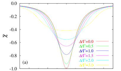
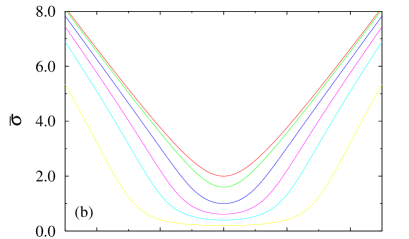
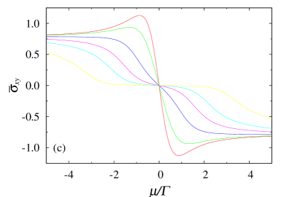
Figure 1: (a) Magnetic susceptibility $\bar{\chi}\equiv\chi 3\pi^{2}c^{2}\hbar^{2}/e^{2}v^{2}$, (b) Conductivity $\bar{\sigma}\equiv\sigma 2\pi h/e^{2}$, and (c) Hall conductivity $\bar{\sigma}_{xy}\equiv\sigma_{xy}4\pi^{2}c/e^{3}v^{2}B$ of the 2D Dirac fermions in the weak-magnetic field, as functions of the scaled chemical potential $\mu/\Gamma$. The results (a), (c) of gapless case ($\Delta=0$) are derived in Ref. Fukuyama_2007 .

Hall effect— Next, we consider the transport properties of this system. The conductivity of the 2D Dirac system is already derived in Ref. Sharapov-G-B . To clarify the derivation of the Hall conductivity $\sigma_{xy}$, we rederive this result first. The conductivity is given by the Kubo formula,

$${\rm Re}\;\sigma_{\mu\nu}=\lim_{\omega\to 0}\frac{{\rm Im}\;\tilde{\Pi}_{\mu\nu}(\bm{0},\omega+{\rm i}\eta)}{\hbar\omega},$$ (21)

where $\tilde{\Pi}_{\mu\nu}(\bm{q},\omega)\equiv\Pi_{\mu\nu}(\bm{q},\omega)-\Pi_{\mu\nu}(\bm{q},0)$. The polarization function in the Matsubara form is given by

$$\Pi_{\mu\nu}(\bm{q},{\rm i}\nu_{m})=\frac{1}{V}\int_{0}^{\beta\hbar}{\rm d}\tau{\rm e}^{{\rm i}\nu_{m}\tau}\langle{\cal T}_{\tau}J_{\mu}(\bm{q},\tau)J_{\nu}(\bm{0},0)\rangle,$$ (22)

$$\tilde{\Pi}_{\mu\nu}(\bm{0},{\rm i}\nu_{m})=-\frac{e^{2}v^{2}}{\beta\hbar V}\sum_{\bm{k}}\sum_{n}{\rm tr}\;\left[{\cal G}\sigma_{\mu}{\cal G}_{+}\sigma_{\nu}\right],$$ (23)

where ${\cal G}_{+}\equiv{\cal G}(\bm{k},\omega_{n}+\nu_{m})$ with $\nu_{m}=2\pi m/\beta\hbar$ being the Matsubara frequency of bosons. The current operator is given by

$$J_{\mu}(\bm{q},\tau)=-ev\sum_{\bm{k}}\Psi^{{\dagger}}(\bm{k}^{+},\tau)\sigma_{\mu}\Psi(\bm{k}^{-},\tau),$$ (24)

where $\bm{k}^{\pm}\equiv\bm{k}\pm\bm{q}/2$. The matrix trace ${\rm tr}\;[\cdots]$ in eq. (23) for $\mu=\nu=x$ is calculated as

$$\frac{2[({\rm i}\tilde{\omega}_{n})({\rm i}\tilde{\omega}_{n}^{+})-\tilde{\Delta}^{2}]}{[({\rm i}\tilde{\omega}_{n})^{2}-v^{2}k^{2}-\tilde{\Delta}^{2}][({\rm i}\tilde{\omega}_{n}^{+})^{2}-v^{2}k^{2}-\tilde{\Delta}^{2}]}\equiv F_{2}({\rm i}\tilde{\omega}_{n},{\rm i}\tilde{\omega}_{n}^{+}),$$ (25)

where $\omega_{n}^{+}\equiv\omega_{n}+\nu_{m}$. The summation of the Matsubara frequency is carried out in the following way,

$$\frac{1}{\beta\hbar}\sum_{n}F_{i}({\rm i}\tilde{\omega}_{n},{\rm i}\tilde{\omega}_{n}^{+})=\frac{-1}{2\pi{\rm i}}\int_{-\infty}^{\infty}{\rm d}\omega f(\hbar\omega)$$ (26)

$$\times[F_{i}(\omega+{\rm i}\tilde{\Gamma},\omega+{\rm i}\nu_{m}+{\rm i}\tilde{\Gamma})-F_{i}(\omega-{\rm i}\tilde{\Gamma},\omega+{\rm i}\nu_{m}+{\rm i}\tilde{\Gamma})$$

$$+F_{i}(\omega-{\rm i}\nu_{m}-{\rm i}\tilde{\Gamma},\omega+{\rm i}\tilde{\Gamma})-F_{i}(\omega-{\rm i}\nu_{m}-{\rm i}\tilde{\Gamma},\omega-{\rm i}\tilde{\Gamma})].$$

After expanding eq. (26) in the linear order of ${\rm i}\nu_{m}$ and the partial integration of $\omega$, it follows from eqs. (21) and (23) that the conductivity is calculated as

$$\sigma=\frac{e^{2}}{4\pi^{2}}\int_{-\infty}^{\infty}{\rm d}\omega[-f^{\prime}(\hbar\omega)]{\cal A}_{2}(\hbar\omega,\Gamma,\Delta),$$ (27)

$${\cal A}_{2}(x,\Gamma,\Delta)\equiv$$

$$\frac{\Gamma^{2}-\Delta^{2}+x^{2}}{2\Gamma|x|}\left(\frac{\pi}{2}-{\rm Tan}^{-1}\frac{\Delta^{2}+\Gamma^{2}-x^{2}}{2\Gamma|x|}\right)+1.$$ (28)

Here the last term in eq. (28) stems from the first and forth terms in eq. (26) where two frequencies have the same analytic properties, while the other terms originate from the second and the third terms. At zero temperature, $f^{\prime}(x)=-\delta(x-\mu)$, we have $\sigma=\frac{e^{2}}{2\pi h}{\cal A}_{2}(\mu,\Gamma,\Delta)$ which is derived in Ref. Sharapov-G-B . The chemical potential dependence of the conductivity is shown in Fig. 1(b). In the limit $\mu/\Gamma\to 0$, we have the minimal conductivity, $\sigma_{\rm min}=\frac{e^{2}}{\pi h}(1+\Delta^{2}/\Gamma^{2})^{-1}$. The dependence of the magnetic field $B$ can be calculated in the similar way of $\sigma_{xy}$ which is discussed below [eq. (29) for $(\mu,\nu)=(x,x)$]. One can show, however, that the conductivity has no $B$-dependence in the linear order.

The Hall conductivity $\sigma_{xy}$ in a weak magnetic field is obtained in the following wayFukuyama-E-W ; Fukuyama_2006 : The Fourier expansion of the vector potential is chosen as $\bm{A}(\bm{r})=\bm{A}_{\bm{q}}{\rm e}^{{\rm i}\bm{q}\cdot\bm{r}}$. Then by the perturbative expansion of eq. (22) in terms of the Hamiltonian in the magnetic field ${\cal H}-\bm{A}_{\bm{q}}\cdot\bm{J}(-\bm{q})/c$, $\sigma_{xy}$ is given by the three point correlation function, and the linear term of the magnetic field $B={\rm i}(q_{x}A_{\bm{q}}^{y}-q_{y}A_{\bm{q}}^{x})$ is obtained by the $\bm{q}$ expansion of the Green function $\partial_{k_{\mu}}{\cal G}=v{\cal G}\sigma_{\mu}{\cal G}$ as,

$$\Pi_{\mu\nu}(\bm{q},{\rm i}\nu_{m})=-\sum_{\alpha=x,y}\frac{A_{\bm{q}\alpha}}{c\hbar}\frac{1}{V}\int_{0}^{\beta\hbar}{\rm d}\tau\int_{0}^{\beta\hbar}{\rm d}\tau^{\prime}$$

$$\times{\rm e}^{{\rm i}\nu_{m}\tau}\langle{\cal T}_{\tau}J_{\mu}(\bm{q},\tau)J_{\alpha}(-\bm{q},\tau^{\prime})J_{\nu}(\bm{0},0)\rangle,$$ (29)

$$\tilde{\Pi}_{\mu\nu}(\bm{0},{\rm i}\nu_{m})=-{\rm i}\frac{B}{c\hbar}\frac{e^{3}v^{4}}{2}\frac{1}{V\beta\hbar}\sum_{\bm{k},n}$$

$$\times{\rm tr}\;[\sigma_{\mu}{\cal G}_{+}\sigma_{x}{\cal G}_{+}\sigma_{\nu}{\cal G}\sigma_{y}{\cal G}-\sigma_{\mu}{\cal G}_{+}\sigma_{y}{\cal G}_{+}\sigma_{\nu}{\cal G}\sigma_{x}{\cal G}$$

$$+\sigma_{\mu}{\cal G}_{+}\sigma_{x}{\cal G}_{+}\sigma_{y}{\cal G}_{+}\sigma_{\nu}{\cal G}-\sigma_{\mu}{\cal G}_{+}\sigma_{y}{\cal G}_{+}\sigma_{x}{\cal G}_{+}\sigma_{\nu}{\cal G}$$

$$+\sigma_{\mu}{\cal G}_{+}\sigma_{\nu}{\cal G}\sigma_{x}{\cal G}\sigma_{y}{\cal G}-\sigma_{\mu}{\cal G}_{+}\sigma_{\nu}{\cal G}\sigma_{y}{\cal G}\sigma_{x}{\cal G}].$$ (30)

The matrix trace ${\rm tr}\;[\cdots]$ for $(\mu,\nu)=(x,y)$ in eq. (30) becomes

$$\frac{-4[({\rm i}\tilde{\omega}_{n})^{2}-({\rm i}\tilde{\omega}_{n}^{+})^{2}][({\rm i}\tilde{\omega}_{n})({\rm i}\tilde{\omega}_{n}^{+})-\tilde{\Delta}^{2}]}{[({\rm i}\tilde{\omega}_{n})^{2}-v^{2}k^{2}-\tilde{\Delta}^{2}]^{2}[({\rm i}\tilde{\omega}_{n}^{+})^{2}-v^{2}k^{2}-\tilde{\Delta}^{2}]^{2}}\equiv F_{3}({\rm i}\tilde{\omega}_{n},{\rm i}\tilde{\omega}_{n}^{+}).$$ (31)

Using eq. (26), the Hall conductivity is obtained as in the same way of the conductivity $\sigma$:

$$\sigma_{xy}=-\frac{e^{3}v^{2}B\hbar}{4\pi^{2}c}\int_{-\infty}^{\infty}{\rm d}\omega[-f^{\prime}(\hbar\omega)]{\cal A}_{3}(\hbar\omega,\Gamma,\Delta),$$ (32)

$${\cal A}_{3}(x,\Gamma,\Delta)\equiv\frac{\Gamma^{2}-\Delta^{2}+x^{2}}{4\Gamma^{2}x|x|}\left(\frac{\pi}{2}-{\rm Tan}^{-1}\frac{\Delta^{2}+\Gamma^{2}-x^{2}}{2\Gamma|x|}\right)$$

$$+\frac{1}{(\Gamma^{2}+x^{2}+\Delta^{2})^{2}-4\Delta^{2}x^{2}}\left(\frac{(\Delta^{2}-x^{2})^{2}-\Gamma^{4}}{2\Gamma x}+\frac{4\Gamma x}{3}\right),$$ (33)

where the last term of ${\cal A}_{3}$ which is proportional to $\frac{4\Gamma x}{3}$ stems from the first and the forth terms in eq. (26). At zero temperature, we have $\sigma_{xy}=-\frac{e^{3}v^{2}B}{4\pi^{2}c}{\cal A}_{3}(\mu,\Gamma,\Delta)$. The chemical potential dependence of the Hall conductivity is shown in Fig. 1(c). In the dirty limit $\Gamma\to\infty$, and $\Delta,\mu\to 0$, the Drude-Zener formula is obtained with $\Gamma=\hbar/2\tau$, where $\tau$ is the mean-free time of qusiparticles. This is consistent with the result obtained by formalism of the Landau quantizationGusynin-S_2006 .

Thermal Hall effect— Finally, we consider the thermal conductivity. The thermal transport of the Dirac system is discussed in the same way of Refs.Gusynin-S_2005a ; Sharapov-G-B ; Ferrer-G-I : For the Hamiltonian density

$$\varepsilon(\bm{r})\equiv\Psi^{{\dagger}}(\bm{r})\hat{\mathcal{H}}_{0}\Psi(\bm{r}),$$ (34)

where the differentiation operator in the one particle Hamiltonian (1) is replaced as $\partial_{\alpha}\to(\partial_{\alpha}-{\displaystyle\mathop{\partial_{\alpha}}^{\leftarrow}})/2$, by the partial integration of eq. (2). Then the time derivative of the local energy is given by

$$\dot{\varepsilon}=\dot{\Psi}^{{\dagger}}\hat{\mathcal{H}}_{0}\Psi+\Psi^{{\dagger}}\hat{\mathcal{H}}_{0}\dot{\Psi}.$$ (35)

The energy current $\bm{J}_{E}$ is determined so that it satisfies the following continuum equation,

$$\dot{\varepsilon}+\nabla\cdot\bm{J}_{E}=0.$$ (36)

Thus we obtain

$$J_{E}^{\alpha}={\rm i}\frac{v}{2}(\Psi^{{\dagger}}\sigma_{\alpha}\dot{\Psi}-\dot{\Psi}^{{\dagger}}\sigma_{\alpha}\Psi).$$ (37)

The current-energy ($\Pi_{\mu\nu}^{CE}$) and the energy-energy ($\Pi_{\mu\nu}^{EE}$) correlation functions are defined as in the same way of eq. (22). These correlation functions have similar structure of the current-current correlation function:

$$\lim_{\omega\to 0}\frac{\beta{\rm Im}\;\tilde{\Pi}_{xy}^{CE}(\bm{0},\omega+{\rm i}\eta)}{\hbar\omega}$$

$$=-\frac{e^{2}v^{2}B}{4\pi^{2}c}\int_{-\infty}^{\infty}{\rm d}xf^{\prime}(x)[\beta(x-\mu)]{\cal A}_{3}(x,\Gamma,\Delta),$$ (38)

$$\lim_{\omega\to 0}\frac{\beta^{2}{\rm Im}\;\tilde{\Pi}_{xy}^{EE}(\bm{0},\omega+{\rm i}\eta)}{\hbar\omega}$$

$$=\frac{ev^{2}B}{4\pi^{2}c}\int_{-\infty}^{\infty}{\rm d}xf^{\prime}(x)[\beta(x-\mu)]^{2}{\cal A}_{3}(x,\Gamma,\Delta).$$ (39)

In the zero temperature limit, using the relation $\int_{-\infty}^{\infty}f^{\prime}(x)[\beta(x-\mu)]^{n}{\rm d}x=1$ ($n=0$), $0$ ($n=\mbox{odd}$), $2n!(1-2^{-n+1})\zeta(n)$ ($n=\mbox{even}\geq 2$), it turns out that eq. (38)$=0$ and eq. (39)$=-\frac{\pi^{2}}{3}\frac{ev^{2}B}{4\pi^{2}c}{\cal A}_{3}(\mu,\Gamma,\Delta)$ where $\zeta(2)=\pi^{2}/6$ is used. Since the thermopower related to $\Pi^{CE}$ does not contribute to the thermal Hall conductivity $\kappa_{xy}$, the Wiedemann-Franz law $\kappa_{xy}/\sigma_{xy}T=(\pi^{2}/3)(k_{\rm B}/e)^{2}$ is satisfied for the Hall and the thermal Hall conductivities in the low temperature limit.

Summary— We have discussed the magnetic susceptibility, the Hall conductivity and the thermal Hall conductivity of the 2D Dirac fermions in the weak magnetic field. We have shown that strong diamagnetism appears even in the gapped system if the Fermi energy is in the middle of the gap. We have also shown that the magnetic susceptibility derived by the weak magnetic field formalism is equivalent with that of the Landau quantization with the Euler-Maclaurin formula. The other results including the Hall conductivity are also consistent with those of the Landau quantization formalism.

Acknowledgment— The author is grateful to Hidetoshi Fukuyama for many helpful guidances and fruitful discussions. He also thanks Shunsuke Furukawa for discussions.

References

(1)
K. S. Novoselov et al., Nature (London) 438, 197 (2005).
(2)
Y. Zhang et al., Nature (London) 438, 201 (2005).
(3)
Y. Zheng and T. Ando, Phys. Rev. B 65, 245420 (2002).
(4)
V. P. Gusynin and S. G. Sharapov,
Phys. Rev. Lett. 95, 146801 (2005).
(5)
V. P. Gusynin and S. G. Sharapov,
Phys. Rev. B 73, 245411 (2006)
(6)
N. H. Shon and T. Ando,
J. Phys. Soc. Jpn. 67, 2421 (1998).
(7)
K. Ziegler, cond-mat/0701300, and references therein.
(8)
S. Katayama, A. Kobayashi, and Y. Suzumura,
J. Phys. Soc. Jpn 75, 054705 (2006).
(9)
A. Kobayashi, S. Katayama, Y. Suzumura, and H. Fukuyama,
to appear in J. Phys. Soc. Jpn.
(10)
X. Yang and C. Nayak,
Phys. Rev. B 65, 064523 (2002).
(11)
S. G. Sharapov, V. P. Gusynin, and H. Beck,
Phys. Rev. B 67, 144509 (2003).
(12)
H. Fukuyama, cond-mat/0703010, to appear in J. Phys. Soc. Jpn.
(13)
H. Fukuyama, Prog. Theor. Phys. 45, 704 (1971).
(14)
J. M. Luttinger and W. Kohn,
Phys. Rev. 97, 869 (1955).
(15)
H. Fukuyama, H. Ebisawa, and Y. Wada,
Prog. Theor. Phys. 42, 494 (1969).
(16)
H. Fukuyama, Ann. Phys. 15, 520 (2006).
(17)
V. P. Gusynin and S. G. Sharapov,
Phys. Rev. B 71, 125124 (2005).
(18)
E. J. Ferrer, V. P. Gusynin, and V. de la Incera,
Eur. Phys. J. B 33, 397 (2003).