Interaction-Induced Adiabatic Cooling for Antiferromagnetism in Optical Lattices

Abstract

In the experimental context of cold-fermion optical lattices, we discuss the possibilities to approach the pseudogap or ordered phases by manipulating the scattering length or the strength of the laser-induced lattice potential. Using the Two-Particle Self-Consistent Approach as well as Quantum Monte Carlo simulations, we provide isentropic curves for the two- and three-dimensional Hubbard models at half-filling. These quantitative results are important for practical attempts to reach the ordered antiferromagnetic phase in experiments on optical lattices of two-component fermions. We find that adiabatically turning on the interaction in two dimensions to cool the system is not very effective. In three dimensions, adiabatic cooling to the antiferromagnetic phase can be achieved in such a manner although the cooling efficiency is not as high as initially suggested by Dynamical Mean-Field Theory. Adiabatic cooling by turning off the repulsion beginning at strong coupling is possible in certain cases.

I Introduction

One of the most exciting possibilities opened by research on cold atoms in optical traps is to study in a controlled manner model Hamiltonians of interest to condensed matter physics. For example, high on the list of questions that can in principle be answered by these model systems is whether high-temperature superconductivity can be explained by the two-dimensional Hubbard model away from half-filling. Jaksch:2004 ; Hofstetter:2002 As a first step towards achieving this goal, the antiferromagnetic phase expected at half-filling offers an easier target state that occurs at higher temperature in the phase diagram of cuprate superconductors. Damascelli:2003 ; Lee:2004

In optical lattices, the two spin species occurring in the Hubbard model are mimicked by atoms in two different hyperfine states. The cooling of these atomic gases necessary to observe ordered states has been discussed before. Blackie:2005 ; Hofstetter:2002 It has been recently pointed out however that there is an additional mechanism, Werner:2006 akin to Pomeranchuck cooling in liquid Helium 3, that is available to help in achieving the temperatures where antiferromagnetism can be observed. In this mechanism, the temperature can be lowered by turning on at constant entropy what amounts to interactions in the Hubbard model (see Ref.(Georges:2007, ) for a review). The original calculations for this effect were done for the Hubbard model using Dynamical Mean-Field Theory (DMFT). Werner:2006 While it is expected that this approach will give qualitatively correct results, accurate predictions are necessary to achieve the practical implementation of this cooling scheme. In the present paper, we present such quantitative predictions for the isentropic curves of both the two- and three-dimensional Hubbard models. We display the results in the usual units for the Hubbard model, but also in the conventional units used in the context of cold atom physics.

Solving the problem for both two- and three-dimensional lattices fulfills several purposes. First, the two-dimensional case is interesting in its own right even if long-range order cannot be achieved at finite temperature in strictly two dimensions (because of the Mermin-Wagner-Hohenberg theorem). Indeed, high-temperature parent antiferromagnetic compounds have a strong two-dimensional character. In addition, even though long-range order cannot be achieved, there is a two-dimensional regime with very strong antiferromagnetic fluctuations that is interesting in itself. In this regime, a pseudogap appears in the single-particle spectral weight that is caused at weak coupling by antiferromagnetic fluctuations that have a correlation length larger than the single-particle de Broglie wavelength. Vilk:1997 ; Tremblay:2006 At strong coupling, the pseudogap appears well before the long antiferromagnetic correlation lengths occur. Kyung:2006 Also, considering both two- and three dimensions sheds additional light on the mechanism for cooling.

The Hubbard model is defined in second quantization by,

$$H=-\sum_{i,j,\sigma}t_{ij}c_{i\sigma}^{\dagger}c_{j\sigma}+U\sum_{i}n_{i\uparrow}n_{i\downarrow}$$ (1)

where $c_{i\sigma}^{\dagger}$ ($c_{i\sigma}$) are creation and annihilation operators for electrons of spin $\sigma$, $n_{i\sigma}=c_{i\sigma}^{\dagger}c_{i\sigma}$ is the density of spin $\sigma$ electrons, $t_{ij}=t_{ji}^{\ast}$ is the hopping amplitude, and $U$ is the on-site repulsion obtained from matrix elements of the contact interaction between atoms in the basis of Wannier states of the optical lattice.Jaksch:2004 ; Georges:2007 We restrict ourselves to the case where only nearest-neighbor hopping $t\$coming from tunneling between potential minima is relevant. In keeping with common practice, $t$ will be the energy unit, unless explicitly stated.

Let us recall the physics of the cooling mechanism proposed in Ref. Werner:2006 . If we denote by $f$ the free-energy per lattice site and $s$ the corresponding entropy, then $s=-\left(\partial f/\partial T\right)_{U}$ and $d=\left(\partial f/\partial U\right)_{T}$ where $d=\langle n_{\uparrow}n_{\downarrow}\rangle$ is the double-occupancy. The chemical potential is kept constant in all partial derivatives without further notice. In the particle-hole symmetric case at half-filling the density is also constant at constant chemical potential. We thus have a Maxwell relation

$$\left(\frac{\partial s}{\partial U}\right)_{T}=-\left(\frac{\partial d}{\partial T}\right)_{U}.$$ (2)

Following Ref. Werner:2006 , the shape of the isentropic curves $s\left(T_{i}\left(U\right),U\right)=cst$ can be deduced by taking a derivative of the last equation and using the Maxwell relation Eq.(2)

$$c\left(T_{i}\right)\left(\frac{\partial T_{i}}{\partial U}\right)_{s}=T_{i}\left(\frac{\partial d}{\partial T}\right)_{U}$$ (3)

where $c\left(T_{i}\right)=T\left(\partial s/\partial T\right)_{U}$ is the specific heat. If $\left(\partial d/\partial T\right)_{U}$ is negative at small $U,$ then $\left(\partial T_{i}/\partial U\right)_{s}$ will be negative and hence it will be possible to lower the temperature at constant entropy by increasing $U.$ Generally, double occupancy increases with temperature so $\left(\partial d/\partial T\right)_{U}$ is positive, but it does happen that $\left(\partial d/\partial T\right)_{U}$ is negative, leading to a minimum at some temperature. This result may seem counterintuitive. Indeed, at strong coupling, namely for interaction strength much larger than the bandwidth, such a phenomenon does not occur. Double occupancy is already minimum at zero temperature. It only increases with increasing temperature. At weak coupling however, when the temperature is large enough that it allows states to be occupied over a large fraction of the whole Brillouin zone, the electrons may become more localized than at lower temperature. An alternate way to understand this minimum is to notice that it occurs when the thermal de Broglie wavelength is of the order of the lattice spacing: Lemay:2000 At larger temperatures, double-occupancy increases because of thermal excitation while at lower temperature the plane-wave nature of the states becomes more apparent and double occupancy also increases. The minimum in $\left(\partial d/\partial T\right)_{U}$ has been observed in DMFT Georges:1996 ; Werner:2006 and also very weakly in Quantum Monte Carlo (QMC) simulations of the two-dimensional model at $U=4t$ (see Figure 3 of Ref. Paiva:2001 ) while in the Two-Particle Self-Consistent (TPSC) approach Vilk:1997 ; Allen:2003 ; Tremblay:2006 that we employ along with QMC, very shallow minima are observed in three dimensions and are barely observable in two dimensions depending on the value of $U.$ Dare:2000 ; Lemay:2000 ; Kyung:2003a ; Roy:2006 As we shall see, in three dimensions a minimum in $\left(\partial d/\partial T\right)_{U}$ is also predicted by second-order perturbation theory. Lemay:2000

In the next section we discuss the two methods that we use, emphasizing the points that are specific to this problem. Then we present the results for the constant entropy curves in two and three dimensions and conclude. Two appendices present calculational details for the entropy curves in limiting cases.

II Methodology

In this section we give methodological details that are specific to this work, referring to the literature for more detailed explanations of the QMC and TPSC approaches.

II.1 Quantum Monte Carlo simulations

In two dimensions we perform QMC simulations following the Blankenbecler-Sugar-Scalapino-Hirsch (determinantal) algorithm. Blankenbecler:1981 The standard formula to obtain the entropy consists in integrating the specific heat. However, the evaluation of the latter quantity involves a numerical derivative. To avoid differentiating data that contains statistical uncertainty, we follow Ref. Werner:2006 and perform an integration by parts to compute the entropy from the energy density $e$

$$s\left(\beta,U\right)=\ln 4+\beta e\left(\beta,U\right)-\int_{0}^{\beta}e\left(\beta^{\prime},U\right)d\beta^{\prime}$$ (4)

with $\beta=1/T$ in units where the Boltzmann constant equals unity. This uses the fact that the entropy at infinite temperature is known exactly. The integral is calculated from the trapezoidal rule on a grid of about twenty points spread on a logarithmic scale that extends from $\beta=0$ to $\beta$ of order $5$ depending on the cases. Each data point is obtained by up to $15\times 10^{6}$ measurements for the $4\times 4$ lattices and $10^{6}$ measurements for $8\times 8$. By comparing with the known result at $U=0,$ we deduce that the error on the integral is of order $2$ to $3\%$ at most at the lowest temperatures. At large values of $U,$ the systematic error due to the discretization of the imaginary time can be quite large. We checked with $U=14$, $\Delta\tau=1/10$, $1/20$ and $1/40$ (in units $t=1$ which we adopt from now on) that $\Delta\tau=1/10$ and $1/20$ suffice for an accurate $\Delta\tau\rightarrow 0$ extrapolation.

Size dependence becomes important at low temperature. These effects can be estimated from the $U=0$ case. Paiva:2001 The usual formula for the entropy

$$s\left(T,U=0\right)=-\frac{2}{N}\sum_{\mathbf{k}}\left(f\ln f+\left(1-f\right)\ln\left(1-f\right)\right)$$ (5)

with $N=L\times L$ (and $L$ even) the number of sites and $f$ the Fermi-Dirac distribution, leads to a residual entropy at $T=0$ given by

$$s\left(0,0\right)=\frac{2L-2}{L^{2}}\ln 4$$ (6)

which does vanish for $L\rightarrow\infty$ but which gives important contributions for finite $L.$ For example, for $L=4,$ we have $s=0.52,$ compared with $\ln 4=1.386$ at $T=\infty$. This entropy is easily understood by counting the number of ways to populate the states that are right at the Fermi surface of the finite lattice in the half-filled Hubbard model. Note-Degenerescence At $T=0.3,$ one can check that the relative error between the $4\times 4$ lattice and the infinite lattice is about $30\%$ while for the $8\times 8$ lattice it is about $5\%$. At $T=0.5,$ the finite size error for the $8\times 8$ lattice is negligible while it is about $5\%$ for the $4\times 4$ lattice. Since in this work we concentrate on high-temperature results, this will in general not be a problem in QMC. The TPSC calculations can be performed in the infinite-size limit and for a finite-size lattice.

II.2 Two-Particle Self-Consistent Approach

The TPSC approach has been extensively checked against QMC approaches in both two Vilk:1997 ; Tremblay:2006 and three Dare:2000 dimensions. It is accurate from weak to intermediate coupling, in other words for $U$ less than about $3/4$ of the bandwidth, namely $U=6$ in $d=2$. The double occupancy is one of the most accurate quantities that can be calculated at the first step of the TPSC calculation using sum rules. Hence, we can compute the entropy directly by integrating the Maxwell relation Eq.(2) in the thermodynamic limit, or for a finite-size system, using the known value of the entropy at $U=0,$ Eq.(5), to determine the integration constant. Earlier results obtained with TPSC for the double occupancy may be found for example in Refs. Vilk:1997 ; Dare:2000 ; Kyung:2003a . Issues of thermodynamic consistency have been discussed in Ref. Roy:2002 .

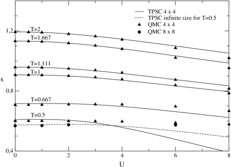
Figure 1: Comparison of TPSC and QMC results for the entropy as a function of $U$ for different temperatures. Solid lines are for TPSC $4\times 4,$ triangles for QMC $4\times 4.$ The dashed line is the TPSC result for the infinite-size lattice limit for $T=0.5$. Also shown by filled circles for this temperature, are the results for QMC $8\times 8.$

Fig. 1 compares the entropy obtained with TPSC (solid and dashed lines) and with QMC (symbols) as a function of $U$ in $d=2$ for different temperatures. The QMC calculations are for a $4\times 4$ system except for $T=0.5$ where we also show results for $8\times 8.$ The TPSC calculations are presented for both $4\times 4$ (solid line) and infinite size limit (dashed line for $T=0.5$). Down to $T=2/3,$ the results for the $4\times 4$ QMC and $4\times 4$ TPSC agree to better than a few percent for $U<6$. One can verify from Fig. 1 that at $T=0.5$ for $U<6,$ infinite-size limit TPSC and $8\times 8$ QMC results agree remarkably, the worse disagreement being less that $10\%$ at $U=6$. This is expected from the fact that according to the discussion of the previous section, finite-size effects are negligible in an $8\times 8$ lattice in this temperature range. Fig. 6 in the following section will compare TPSC estimates of the Néel temperature with the latest QMC calculations Staudt:2000 in $d=3$. There again, $U$ equals $3/4$ of the bandwidth seems to be the limit of validity. We stress that TPSC is in the $N=\infty$ universality class Dare:1996 so that details may differ with the exact result in the critical region. Nevertheless, it has been checked that even with correlation lengths of order $10$ or more, the results are still quite accurate.

III Results

III.1 Two dimensions

The data that is directly extracted from the QMC calculation is the total energy per site. The entropy extracted from this data by numerical integration, Eq.(4), is plotted as a function of $\beta U/4=U/\left(4T\right)$ on a logarithmic scale for different values of $U$ in Fig. 2 along with the exact atomic (single site) limit

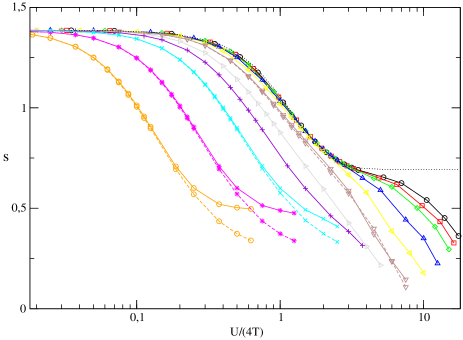
Figure 2: (Color online) Entropy as a function of $\beta U/4$. From bottom to top, increasing values of $U=0.5,1,2,3,4,6,8,10,12,13,14$ are displayed. Solid lines are for $4\times 4$ lattice and dashed lines for $8\times 8$ lattice. Dotted line is the exact atomic limit result for $U=14$.

$$s_{atomic}\left(\beta,U\right)=\ln\left(4\cosh\left(\frac{\beta U}{4}\right)\right)-\frac{\beta U}{4}\tanh\left(\frac{\beta U}{4}\right).$$ (7)

Also plotted in Fig. 2 are the data for an $8\times 8$ lattice when $U=0.5,1,2,$ $6$. One can check that for $\beta<1$ $\left(4T>W/2\right)$ and $U>W,$ where $W=8$ is the bandwidth, the above simple formula describes the data to better than $4\%$ accuracy. This is consistent with earlier QMC results Paiva:2001 that found that for $U=10$ the specific heat above $T=1$ is well described by the atomic limit. Limiting cases of the above formula are interesting. At infinite temperature, $\beta U=0,$ one recovers the expected $\ln 4$ entropy with the first correction given by

$$s_{atomic}\left(\beta,U\right)=\ln 4-\left(\beta U\right)^{2}/32+\emph{O}\left(\left(\beta U\right)^{4}\right).$$ (8)

In the $\beta U=\infty$ limit, only spin entropy is left so the atomic limit result Eq.(7) reduces to $\ln 2.$

At small values of the entropy, the curves in Fig. 2 at small $U$ have a break. This can be understood as a finite-size effect given that $s\sim 0.5$ is the residual entropy for a $4\times 4$ lattice at $U=0.$ Lower entropies can be reached at larger $U$ without size effects since $U$ lifts the Fermi surface degeneracy. Note-Degenerescence In addition, the results for a $8\times 8$ lattice and small $U$ shown by dashed lines do extend to lower values of the entropy.

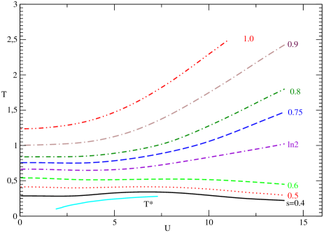
Figure 3: (Color online) Isentropic curves for $d=2$ extracted from QMC simulations, including the results of the $8\times 8$ lattice when they differ from those of the $4\times 4$. Increasing values of $s$ are displayed from bottom to top. The first line above the horizontal axis is the value of the crossover temperature $T^{*}$ determined from TPSC. It stops at strong coupling where TPSC ceases to be accurate.

Isentropic curves in Fig. 3 are plotted in units of $T/t$ and $U/t$. They are obtained from interpolation of the QMC entropy, except for the first line above the horizontal axis that represents the value of the crossover temperature $T^{*}$ obtained from TPSC. tstar As discussed above, the data in the upper right sector $U>8,$ $T>1$ are quite accurately explained by the atomic limit. It should be stressed that the slow variation of entropy with $T$ and $U$ translates into inaccuracies in the interpolation of the isentropic curves that can reach about $10\%$ in this regime. When $U<4T$ and $W<8T$, one would expect that the high-temperature perturbative result

$$s\left(\beta,U\right)=s\left(\beta,0\right)-\frac{1}{32}\left(\beta U\right)^{2}+\emph{O}\left(\left(\beta U\right)^{4}\right)+\emph{O}\left(\beta^{3}U^{2}W\right)$$ (9)

derived in the appendices should describe well the QMC data. In fact, the term $\emph{O}\left(\beta^{3}U^{2}W\right)$ in the range of temperatures shown seems to be large enough to essentially cancel the effect of the leading $\left(\beta U\right)^{2}$ term. The QMC isentropic curves leave the $U=0$ axis with essentially a zero curvature and are extremely well described by the non-interacting result $s\left(\beta,0\right)$ in Eq.(5). More specifically, for $T>1,$ $U\leq 4$ the difference between QMC and $s\left(\beta,0\right)$ is less than $3\%$. At $T>1$ again, the crossover between the atomic limit value Eq.(7) and the non-interacting value Eq.(5) occurs around $U=6$ where both results differ at $T=1$ by about $10\%$ from the QMC results. That regime does not lead to an isentropic decrease in temperature concomitant with an increase in $U$. In the non-trivial regime where the entropy may fall with increasing $U$ according to DMFT, Werner:2006 it is known quite accurately that for $U=4,$ the pseudogap regime where antiferromagnetic fluctuations are large begins around $T=0.22.$ Fig. 3 shows that Werner:2006 contrary to the three dimensional results of the following section, it does not appear possible to lower the temperature substantially by following an isentropic curve from the $U=0$ limit. Only a small effect is observed. Even near $T=0.5,$ the isentropic curve deviates only a little bit from the non-interacting value but it is quite close to it up to $U$ about $6$ where a slight downturn in the isentropic curve occurs. NoteCrossover The flat behavior observed in this regime is confirmed by TPSC calculations: the disagreement between the two methods down to $T=0.2$ is inside the error induced by $\beta$-integration of QMC results. The nearly horizontal isentropic is not surprising given that the minimum in the temperature dependent double occupancy found earlier is shallow in both TPSC Dare:2000 ; Lemay:2000 ; Kyung:2003a ; Roy:2006 and QMC Roy:2002 ; Roy:2006 ; Brillon:2007 calculations. A very small minimum in $d\left(T,U=4\right)$ has been found by extrapolating double-occupancy (local moment) to the infinite size limit in the QMC calculations of Ref.  Paiva:2001 . Note that entry into the pseudogap (fluctuating) regime corresponds to a rapid fall of $d$ as $T$ decreases. Dare:2000 ; Lemay:2000 ; Kyung:2003a ; Roy:2006 ; Paiva:2001 In fact the anticipation of this downfall seems to interfere with the formation of the minimum found in higher dimension. In the regime where $d$ decreases rapidly as temperature decreases, temperature should increase with $U$ along isentropic curves, going in the direction opposite to the one that would be useful for cooling from the non-interacting regime to the fluctuating phase.

From the large $U$ region, an isentropic decrease in $U$ may also lead to a decrease in $T,$ as is obvious already from the atomic limit result Eq.(7). In the two-dimensional case considered here, the results of the QMC calculation in Fig. 3 show that for $s<0.6$, adiabatic cooling from large $U$ is not possible. All the temperatures along the $s=0.6$ isentropic curves are above the fluctuation regime. Hence that regime apparently cannot be reached along a single adiabatic curve starting from large $U$ and large $T.$ Note however the $s=\ln 2$ isentropic curve in Fig. 3. It corresponds to the high temperature spin entropy in the large $U$ limit ($U\gg T\gg 4t^{2}/U$). NoteDeg If one can trap only one of the two atomic species per lattice site at random in the large $U$ regime, we are in the $\ln 2$ entropy case. The lowest temperature that can be reached by following this isentropic curve is about a factor two above the maximum temperature where the strongly fluctuating (pseudogap) regime occurs.

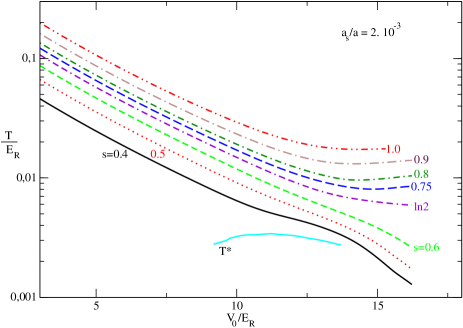
Figure 4: (Color online) Isentropic curves for $d=2$ ($k_{B}=1$) extracted from QMC simulations, expressed in experimental units (see text).

We now discuss the isentropic curves in terms of experimental parameters and units. In optical lattices, lasers create a periodic potential defined by a period $a=\lambda/2$, ( $\lambda$ is the laser wavelength) and a depth $V_{0}$. The energy unit conventionally used in this context is the recoil energy: $E_{R}=\frac{2\pi^{2}\hbar^{2}}{m\lambda^{2}}$, where $m$ is the mass of the fermion. To create a two-dimensional optical lattice, there is a third standing wave confining the 2D system with a depth that is large enough to prevent out-of-plane tunneling. This leads to a 2D on-site energy $U$ related to the geometric mean of the confinement strengths $U/E_{R}=4\sqrt{2\pi}(a_{s}/\lambda)(V_{\perp}/E_{R})^{1/4}(V_{0}/E_{R})^{1/2}$ where $a_{s}$ is s-wave scattering length. Zwerger:2003 ; Kollath:2006 As explained in Refs. Werner:2006, ; Georges:2007, , there is a relation to fulfill between $a_{s}$, $V_{0}$ and $a$ for the one-band Hubbard model to be an accurate description of cold atoms in optical traps.

The best way to change only the interaction strength for adiabatic cooling is to change the scattering length, as can be done by tuning through a Feshbach resonance. If only the scattering length is changed, the shape of the adiabatic curves will be as in Fig. 3. Only the scales need to be changed. All energies in that plot are in units ($k_{B}=1$) of hopping $t$ which is related to recoil energy and potential strength through $t=E_{R}(4/\sqrt{\pi})(V_{0}/E_{R})^{3/4}\exp{\Bigl{(}-2\sqrt{V_{0}/E_{R}}\Bigr{)}}$.Zwerger:2003

We can also change $U$ by changing the potential strength $V_{0}$ but clearly this changes also the hopping $t$. Thus for quantitative purposes, we also display the preceding isentropic curves in the $(V_{0}/E_{R},T/E_{R})$ plane, rather than in the $(U/t,T/t)$ plane. This change in coordinates is discussed in Appendix A. It has a strong influence on the shape of the isentropic curves as can be seen in Fig. 4, obtained for the value $a_{s}/a=2\ 10^{-3}$ and $U=E_{R}4\sqrt{2\pi}(a_{s}/\lambda)(V_{\perp}/E_{R})^{1/4}(V_{0}/E_{R})^{1/2}$ with $V_{\perp}/E_{R}=30$. Kollath:2006 We also display in this figure the pseudogap temperature $T^{*}$ determined in the TPSC approach. tstar As $V_{0}/E_{R}$ increases, the system cools down along isentropic curves, at least for moderate $V_{0}/E_{R}$ values. For higher values, isentropic curves corresponding to $s>\ln{2}$ eventually bend upwards, while those corresponding to $s<\ln{2}$ bend downwards, in such a way that there is a large domain of temperatures in the vicinity of the large-repulsion spin-entropy value $s=\ln{2}$. This general behavior was also present in Fig. 3, and will be seen in 3D too. We checked than the general appearance does not change for other reasonable values of $a_{s}/a$ compatible with the Hubbard model. Given that the temperature axis is displayed on a logarithmic scale, it thus appears that tuning the potential $V_{0}$ can be very effective in reducing the temperature of the fermions. The general cooling trend is due to the decrease in hopping $t$ associated to an increase in $V_{0}$. Indeed, the ratio of temperature to bandwidth is constant for isentropic curves of non-interacting electrons, hence $T$ decreases monotonically with decreasing $t$ in this case. This is the mechanism discussed in Ref.Blackie:2005 . At $V_{0}<2.3E_{R}$, (not on the figure) heating can also occur. Blackie:2005 The presence of interactions can enhance the cooling compared with the non-interacting case. Werner:2006 ; Georges:2007 However, cooling down the system along an isentropic by increasing $V_{0}$ does not necessarily mean an effective approach of the strongly fluctuating regime of the system: indeed, as can be seen from the figure, if we increase $V_{0}/E_{R}$ further than about 12 the pseudogap region in experimental units moves away towards lower temperatures. Note that $T^{*}$ determined by TPSC is not reliable at large values of $V_{0}/E_{R}$: the limit of validity $\frac{U}{W}\sim\frac{3}{4}$, corresponds to $\frac{V_{0}}{E_{R}}\sim 12$, for our choice of $a_{s}/a$ and $V_{\perp}/E_{R}$. Note-Texp-2D

III.2 Three dimensions

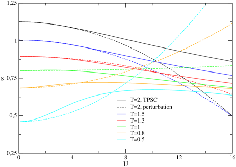
Figure 5: (Color online) Comparisons of full TPSC calculation (solid lines) with second-order perturbation theory (dashed line) for the entropy as a function of $U$ for different temperatures.

To discuss the isentropic curves in 3D, let us go back for a while to usual units and parameters of the Hubbard model. In three dimensions, adiabatic cooling towards the antiferromagnetic phase, starting from small $U$, is possible and quite clearly so. In fact, it occurs at high enough temperature that perturbation theory (Appendix C) suffices to show the effect. This is made clear by Fig. 5 where $\partial s/\partial U$ changes sign from negative to positive on isothermal curves, as $T$ decreases. By Maxwell’s relation Eq.(2), this reflects the change in sign of $\partial d/\partial T$. When the temperature is large enough, the dashed lines from second order perturbation theory agree very well, up to quite large interaction strength, with the solid lines from the full TPSC calculation

The TPSC results for the isentropic curves in three dimensions are exhibited in Fig. 6. In the low-temperature regime $2\pi T/W<1,$ TPSC is strictly valid only in the $U\ll W$ $\left(W=12\right)$ limit. This can be checked by comparing the TPSC Néel temperature with that of the latest QMC calculations, shown by symbols. Staudt:2000 Clearly, the agreement is satisfactory up to $U\simeq 8$ (or $U\simeq 3W/4$ as mentioned before) where the Néel temperature as a function of $U$ saturates according to TPSC but begins to decrease according to QMC.

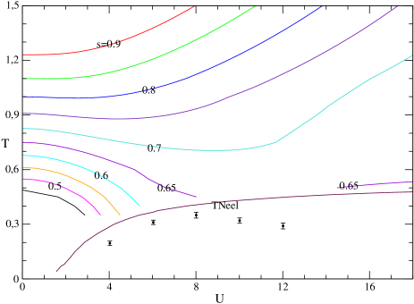
Figure 6: (Color online) Isentropic curves for $d=3$ extracted from TPSC. Increasing values of $s$ are displayed from bottom to top. The lowest solid line is the Néel temperature. Symbols are the results of QMC calculations taken from Ref.Staudt:2000 .

Despite the fact that TPSC is not valid in the atomic limit, it seems to recover the correct result at high-temperature even if $U>W.$ Consider for example $T=1.5.$ That temperature is reached along the $s=0.8$ isentropic around $U=14$ in TPSC and around $U=13$ in DMFT. Werner:2006 Similarly, $T=1.5$ is reached along the $s=0.75$ isentropic for $U\sim 17$ for both TPSC and DMFT. The corresponding atomic limit results, that are dimension independent, are that $s\left(T=1.5,U=11\right)\sim 0.80$ and $s\left(T=1.5,U=14\right)\sim 0.75.$ TPSC is closer to DMFT than to the high-temperature atomic limit, suggesting that both approaches take into account the same physics at $U$ large in the high-temperature limit. Note however that the DMFT and TPSC results are different at $U=0$ because a model density of states is used in DMFT instead of the one following from the exact dispersion relation used in TPSC.

As in the two-dimensional case, the value of the entropy at $T>1$ and $U<W$ is almost independent of $U.$ Contrary to the two dimensional case however, there is a region, namely for $s\lesssim 0.65$, where cooling along isentropic curves down to the interesting regime is possible. Cooling however is from $T\sim 0.75$ to the maximum Néel temperature, $T\sim 0.4.$ DMFT predicted cooling to the Néel temperature beginning around $T\sim 1.1.$

The possibility of adiabatically cooling all the way to the Néel temperature starting from large $U$ is also discussed in Ref. Werner:2006 . For this one needs two conditions. First, the entropy at the maximum Néel temperature has to be larger than the entropy of the Heisenberg antiferromagnet. This condition is satisfied according to Fig. 6 since the entropy at the maximum Néel temperature is around $s_{\max}=0.65$ while the entropy of the Heisenberg antiferromagnet is a constant $s_{H}$ estimated in Ref. Werner:2006 to be about $50\%$ smaller than $\ln 2.$ This would mean that there is indeed a maximum in the value of the entropy at the Néel température plotted as a function of $U.$ That maximum would be even more pronounced than that sketched in Fig. 3 of Ref. Werner:2006 . The second condition to be satisfied is that the temperature should decrease as $U$ decreases along isentropic curves in the range $s_{H}<s<s_{\max}$. TPSC cannot tell whether this condition is satisfied since for temperatures less than roughly unity at strong coupling $U>8$ the TPSC results cannot be fully trusted.

Incidentally, if one takes the TPSC results seriously up to $T\sim 0.7,$ then it is not possible to cool all the way to Néel temperature along the $s=\ln 2=0.69$ “infinite”-temperature $\left(U/T\ll 1\right)$ isentropic curve, contrary to what DMFT suggests, since the minimum in the $s=0.7$ isentropic curve in Fig. 6 is roughly a factor of two above the Néel temperature. As discussed in Ref. Werner:2006 , DMFT does not give an accurate estimate of the entropy at the Néel temperature since the latter is obtained in mean-field. NoteGeorges This is why the $s=0.7$ isentropic curve ends at the Néel temperature in that approximation.

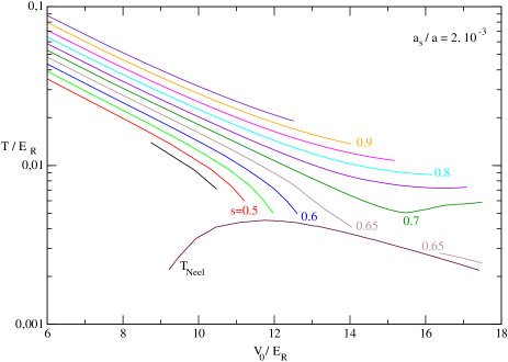
Figure 7: (Color online) Isentropic curves for $d=3$ from TPSC calculations, expressed in experimental units (see text).

Finally, we discuss experimental units. Once again, increasing the scattering length would be the simplest way to implement directly the Pomeranchuck adiabatic cooling discussed in this paper. Indeed varying the scattering length value will span the abscissa axis in Fig.6. All energies in that plot are in units ($k_{B}=1$) of hopping $t$ which is related to recoil energy and potential strength through $t=E_{R}(4/\sqrt{\pi})(V_{0}/E_{R})^{3/4}\exp{\Bigl{(}-2\sqrt{V_{0}/E_{R}}\Bigr{)}}$.Zwerger:2003 The interaction strength on the other hand is $U=E_{R}4\sqrt{2\pi}(a_{s}/\lambda)(V_{0}/E_{R})^{3/4}$.Zwerger:2003

As in the 2D case, we choose to change the potential strength $V_{0}$, that modifies both hopping $t$ and on-site interaction $U$. This is shown in Fig.7 where we display the isentropic curves and the TPSC-determined Néel temperature in the experimental units Note_T_exp . For the figure, we fix $a_{s}/a=2\ 10^{-3}$. Increasing the potential $V_{0}$ is quite efficient to cool down the system in absolute units, but the Néel temperature also recedes. Two trends remain: for $s>\ln{2}$ the cooling is not sufficient to reach the antiferromagnetic region, but a smaller entropy value may do. In these units, the isentropic $s=\ln{2}$ seems ”noisy” for large $V_{0}/E_{R}$ values because, in this region, the entropy surface is flat: this makes the precise location of the isentropic curve difficult to determine.

IV Conclusion

TPSC calculations confirm that the physics of adiabatic cooling by increase of $U$ (as found in Ref. Werner:2006 ) is correct for three dimensions. Our quantitative estimates show a smaller but still appreciable effect. Since it occurs at relatively high temperature, that effect is qualitatively captured already by second order perturbation theory. Adiabatic cooling should help in reaching the Néel antiferromagnetic transition temperature. Reaching the antiferromagnetic phase should be a first step in the study of d-wave superconductivity in optical traps. In two dimensions however, QMC shows that this mechanism is not very effective, making it impractical to reach the low temperature fluctuating regime by this approach.

In both $d=2$ and $d=3$ it is possible to adiabatically cool starting from the large $U$ regime as suggested in Ref. Werner:2006 . However, in $d=2,$ the fluctuating regime cannot be reached along a single adiabatic using this approach. In $d=3,$ although there are encouraging trends, we cannot tell unambiguously with TPSC whether the Néel temperature of the Heisenberg antiferromagnet can be reached by decreasing $U$ along a single adiabatic that starts at high temperature.

In the context of cold fermions, changing the strength of the laser-induced lattice potential changes both hopping $t$ and interaction strength $U$. In units of absolute temperature and potential strength then, the shape of the adiabatic curves are quite different from those in the $T/t$ and $U/t$ units appropriate for the Hubbard model. While the change in $t$ can, for some cases, produce drastic cooling in absolute units, it also changes the shape of the lines for the Néel temperature (in 3D) and the pseudogap temperature (in 2D). We have plotted the results for a given scattering length as examples. Whether a given isentropic curve crosses the Néel or the pseudogap temperature is clearly independent of coordinates. To implement directly the type of interaction driven adiabatic cooling discussed in the present paper, one could change only the interaction strength by manipulating the scattering length with a Feshbach resonance.

Adiabatic cooling away from half-filling and for other cases can be studied with the methods of this paper.

Appendix A Exprimental coordinates for the two-dimensional case

The problem of converting from the theoretical units $\left(U/t,T/t\right)$ to the experimental units $\left(V_{0}/E_{R},T/E_{R}\right)$ is straightforward in three dimensions but it requires some discussion in two dimensions. Since Zwerger:2003 ; Kollath:2006

$$\frac{U}{E_{R}}=4\sqrt{2\pi}\left(\frac{a_{s}}{\lambda}\right)\left(\frac{V_{\bot}}{E_{R}}\right)^{1/4}\left(\frac{V_{0}}{E_{R}}\right)^{1/2}$$ (10)

and

$$\frac{t}{E_{R}}=\frac{4}{\sqrt{\pi}}\left(\frac{V_{0}}{E_{R}}\right)^{3/4}\exp\left(-2\sqrt{\frac{V_{0}}{E_{R}}}\right).$$ (11)

it follows immediately that

$$\frac{U}{t} =\pi\sqrt{2}\left(\frac{a_{s}}{\lambda}\right)\left(\frac{V_{\bot}}{E_{R}}\right)^{1/4}\left(\frac{V_{0}}{E_{R}}\right)^{-1/4}\exp\left(2\sqrt{\frac{V_{0}}{E_{R}}}\right)$$ (12)

$$\frac{T}{t} =\left(\frac{T}{E_{R}}\right)\frac{\sqrt{\pi}}{4}\left(\frac{V_{0}}{E_{R}}\right)^{-3/4}\exp\left(2\sqrt{\frac{V_{0}}{E_{R}}}\right).$$ (13)

For definiteness we choose in this paper $a_{S}/\lambda=10^{-3}$ and $V_{\bot}/E_{R}=30.$ Clearly, $U/t$ is not a monotonic function of $V_{0}$. For a given $U/t$ we have two or zero real values of $V_{0}$ as we now discuss.

For the sake of simplicity, let us define the reduced units

$$u =\frac{U}{t}\left[\pi\sqrt{2}\left(\frac{a_{s}}{\lambda}\right)\left(\frac{V_{\bot}}{E_{R}}\right)^{1/4}\right]^{-1}$$ (14)

$$v_{0} =\sqrt{\frac{V_{0}}{E_{R}}}.$$ (15)

Then, the relation between $u$ and $v_{0}$ becomes

$$u=v_{0}^{-1/2}\exp\left(2v_{0}\right).$$ (16)

This function has a minimum at $v_{0}=1/4.$ The only possible values of $u$ are thus $u\geq 2\sqrt{e}$ and for each such values of $u,$ there are two values of $v_{0},$ one less than $1/4$ and the other one larger than $1/4.$ It is the latter that we consider as the physical value. Indeed, it corresponds to $V_{0}/E_{R}\geq 1/16$ and we know that the Hubbard model is valid only for sufficiently large values of $V_{0}/E_{R}.$ The minimum value of $U/t$ for $V_{\bot}/E_{R}=30$ is about $34a_{s}/\lambda$ which is quite a small value. To solve for $v_{0}\left(u\right),$ it suffices to rewrite Eq.(16) as

$$-\frac{4}{u^{2}}=-4v_{0}\exp\left(-4v_{0}\right).$$ (17)

The solution to $y=x\exp\left(x\right)$ is the Lambert function $W_{k}$ (also known as “product log” function). Since $y\left(x\right)$ is non-monotonic, there exists a family $W_{k}$ of inverse functions. If $U$ is larger or equal to the bound discussed above, then $0>y\geq-1/e$ and $W_{k=-1,0}$ can take real values. The branch $x=W_{-1}\left(y\right)$ has $x\leq-1$, corresponding to $V_{0}/E_{R}\geq 1/16$ that we want to retain. The other branch, $x=W_{0}\left(y\right)$ leads to $x\geq-1$ which we do not consider here. Hence the solution is

$$\frac{V_{0}}{E_{R}} =\left[-\frac{1}{4}W_{-1}\left(-\frac{4}{u^{2}}\right)\right]^{2}$$

$$=\left[-\frac{1}{4}W_{-1}\left(-\frac{t^{2}}{U^{2}}8\pi^{2}\left(\frac{a_{s}}{\lambda}\right)^{2}\left(\frac{V_{\bot}}{E_{R}}\right)^{1/2}\right)\right]^{2}$$ (18)

Appendix B Entropy in the large temperature limit from the self-energy

Consider the large Matsubara frequency (equivalently high-temperature) limit of the self-energy, Vilk:1997

$$\Sigma\left(\mathbf{k,}ik_{n}\right)=Un_{-\sigma}+\frac{U^{2}n_{\sigma}\left(1-n_{-\sigma}\right)}{ik_{n}}+\ldots$$ (19)

This formula is valid when $\pi T$ is larger than the frequency range over which $\Sigma^{R\prime\prime}$ is non-zero. In practice, since in all the diagrams that enter the calculation of the self-energy, $k_{n}=\left(2n+1\right)\pi T$ is compared with $\varepsilon_{\mathbf{k}}$ and there is particle-hole symmetry at half-filling, we may expect that as soon as the Matsubara frequencies are larger than band energies of order $\pm W/2,$ namely $\pi T>W/2,$ then the expansion may apply. This is confirmed by the numerical results in this paper. The expansion should thus be valid for $\pi T\gg 4$ in $d=2,$ and $\pi T\gg 6$ in $d=3$. If, inspired by the exact atomic result Eq.(7) we replace $\pi$ by $4$ we recover the limits of validity mentioned in the text. In addition to this restriction on temperature compared with bandwidth, we note that this asymptotic expansion for the self-energy Eq. (19) is clearly a power series in $U/\pi T$. At half-filling, using the usual canonical transformation to the attractive Hubbard model, we can see that if we absorb the Hartree-Fock term in the definition of the chemical potential then only even powers of $U$ enter the expansion, which makes it convergent even faster. In addition, it turns out that stopping the expansion of $\Sigma\left(\mathbf{k,}ik_{n}\right)$ at $U^{2}/ik_{n}$ at half-filling reproduces the exact result in the atomic limit. Hence, in the special case we are interested in, we expect that this high-temperature expansion $W/2\pi T\ll 1$ is excellent for arbitrary values of $U,$ even if strictly speaking it should be valid only if $U/\pi T\ll 1$ as well.

From the above expression for the self-energy and the sum-rule, Vilk:1997

$$\frac{T}{N}\sum_{n}\sum_{\mathbf{k}}\Sigma\left(\mathbf{k,}ik_{n}\right)G\left(\mathbf{k,}ik_{n}\right)e^{-ik_{n}0^{-}}=U\left\langle n_{\uparrow}n_{\downarrow}\right\rangle$$ (20)

we can extract the double occupancy $d$ that we need to compute the entropy in the high-temperature limit. For the Green function, we again assume that $W/2\pi T\ll 1.$ This means that we can insert in the previous equation

$$G\left(\mathbf{k,}ik_{n}\right)=\frac{1}{ik_{n}-\frac{U^{2}}{4ik_{n}}}.$$ (21)

This clearly neglects band effects that would contribute to order $UW/\left(\pi T\right)^{2}$ to double occupancy. The normalized sum over wave-vectors in the sum-rule Eq.(20) contributes a factor unity while the discrete Matsubara sum can be performed exactly. One finds,

$$-\frac{U}{4}\tanh\left(\frac{U}{4T}\right)=U\left(\left\langle n_{\uparrow}n_{\downarrow}\right\rangle-\left\langle n_{\uparrow}\right\rangle\left\langle n_{\downarrow}\right\rangle\right).$$ (22)

To extract the entropy, it suffices to use Maxwell’s relation Eq.(2) so that

$$s\left(T,U\right) = s\left(T,0\right)-\int_{0}^{U}\frac{\partial\left(-\frac{1}{4}\tanh\left(\frac{U}{4T}\right)\right)}{\partial T}dU$$

$$= s\left(T,0\right)+\ln\left(\cosh\left(\frac{U}{4T}\right)\right)-\frac{U}{4T}\tanh\left(\frac{U}{4T}\right).$$

The above expression Eq.(B) with the exact value for $s\left(T,0\right)$ neglects terms of order $U^{2}W/\left(\pi T\right)^{3}.$ In practice, we found that keeping the non-interacting value of the entropy $s\left(T,0\right)$ in the above formula does not improve the comparison with QMC data in the region where $W/2\pi T\ll 1$ is satisfied, whether $U$ is small or large. When we neglect all band effects compared with temperature, then $s\left(T,0\right)$ can be replaced by $\ln 4$ and we recover the atomic limit result Eq.(7) that can also be found from elementary statistical mechanics. It is the latter result that is useful to understand the data at large values of $U.$

Expansion of $s\left(T,U\right)$ above in powers of $U/4T$ leads to the perturbative result Eq.(9). One can also arrive at this result by directly neglecting higher powers of $U/\pi T$ and $UW/\left(\pi T\right)^{2}$ in the self-energy and Green function,

$$\frac{T}{N}\sum_{n}\sum_{\mathbf{k}}\Sigma\left(\mathbf{k,}ik_{n}\right)G\left(\mathbf{k,}ik_{n}\right)e^{-ik_{n}0^{-}} \simeq \frac{T}{N}\sum_{n}\sum_{\mathbf{k}}\left(Un_{-\sigma}+\frac{U^{2}n_{\sigma}\left(1-n_{-\sigma}\right)}{ik_{n}}\right)\frac{1}{ik_{n}}e^{-ik_{n}0^{-}}$$ (24)

$$= U\left\langle n_{\uparrow}\right\rangle\left\langle n_{\downarrow}\right\rangle-T\sum_{n}\frac{U^{2}}{4\left(2n+1\right)^{2}\left(\pi T\right)^{2}}$$ (25)

$$= U\left\langle n_{\uparrow}\right\rangle\left\langle n_{\downarrow}\right\rangle-\frac{U^{2}}{16T}=U\left\langle n_{\uparrow}n_{\downarrow}\right\rangle$$ (26)

so that

$$s\left(T,U\right) = s\left(T,0\right)-\int_{0}^{U}\frac{\partial\left(-\frac{U}{16T}\right)}{\partial T}dU$$ (27)

$$= s\left(T,0\right)-\frac{U^{2}}{32T^{2}}.$$ (28)

This result, appearing in Eq.(9), keeps all powers in $W/2\pi T,$ the leading term in $U/\pi T$ and neglects $U^{2}W/\left(\pi T\right)^{3}$ and higher orders (the entropy is an even function of $U$ at half-filling). It does not however assume that $U/W<1.$ It is the large temperature here that controls the expansion. In practice we found that the above formula does not lead to a good description of the QMC data in any regime, even small $U$ and large $T$, unless $s\left(T,0\right)\rightarrow\ln 4$ in the large $U$ regime. This suggests that the corrections $\emph{O}\left(\left(\beta U\right)^{4}\right)+\emph{O}\left(\beta^{3}U^{2}W\right)$ are important and in fact cancel the leading one.

Note that in all the results of this section, the dimension occurs only in the value of $W$ and in the value of $s\left(T,0\right).$ The atomic limit is independent of dimension.

Appendix C Second order perturbation theory and TPSC for the entropy

In the limit $U\ll W,$ TPSC reproduces the standard perturbative expression for double occupancy. This can be demonstrated as follows. In TPSC, double occupancy is obtained from the following sum rule and ansatz Vilk:1997 ; Allen:2003

$$n-2\langle n_{\uparrow}n_{\downarrow}\rangle = \frac{T}{N}\sum_{q}\frac{\chi_{0}(q)}{1-\frac{1}{2}U_{sp}\chi_{0}(q)}$$ (29)

$$U_{sp} = U\frac{\langle n_{\uparrow}n_{\downarrow}\rangle}{\langle n_{\uparrow}\rangle\langle n_{\downarrow}\rangle}.$$ (30)

We used short-hand notation for wave vector and Matsubara frequency $q=(\mathbf{q,}iq_{n})$. Since the self-energy is constant in the first step of TPSC, the irreducible susceptibility takes its non-interacting Lindhard value $\chi_{0}(q).$ In a perturbation theory in $U,$ we can expand the right-hand side of the sum rule Eq.(29) and take $U_{sp}=U$ which leads to

$$n-2\langle n_{\uparrow}n_{\downarrow}\rangle = \frac{T}{N}\sum_{q}\left(\chi_{0}(q)+\frac{1}{2}U\chi_{0}^{2}(q)\right)$$ (31)

$$= n-2\langle n_{\uparrow}\rangle\langle n_{\downarrow}\rangle+\frac{1}{2}U\frac{T}{N}\sum_{q}\chi_{0}^{2}(q)$$

or

$$\langle n_{\uparrow}n_{\downarrow}\rangle-\langle n_{\uparrow}\rangle\langle n_{\downarrow}\rangle=-\frac{1}{4}U\frac{T}{N}\sum_{q}\chi_{0}^{2}(q)$$ (32)

which shows, as expected, that double-occupancy is decreased by repulsive interactions compared with its Hartree-Fock value. The above corresponds to the expression obtained from direct perturbation theory for $\langle n_{\uparrow}n_{\downarrow}\rangle-\langle n_{\uparrow}\rangle\langle n_{\downarrow}\rangle$. The entropy can be obtained, as usual, from integration of the Maxwell relation Eq.(2) using the known $s\left(T,U=0\right)$. This is how the perturbative result in Fig. 5 was obtained.

In the high-temperature limit, we recover results of the previous section, as we now proceed to show in two different ways. TPSC at the first level of approximation obeys the sum rule Eq.(20) that expresses a consistency between single-particle and two-particle quantities. The self-energy in the $U/W<1$ and large Matsubara-frequency limit has been found in Ref. Vilk:1997 , Eq.(E.10)

$$\Sigma\left(\mathbf{k,}ik_{n}\right)=Un_{-\sigma}+\frac{U}{ik_{n}}\left(\frac{U_{sp}+U_{ch}}{2}n_{-\sigma}-U_{ch}n_{-\sigma}^{2}+\frac{\left(U_{sp}-U_{ch}\right)}{2}\left\langle n_{\uparrow}n_{\downarrow}\right\rangle\right)+\ldots$$ (33)

In the high-temperature limit $\pi T\gg W/2$ that we are interested in, the classical (zero-frequency) contribution dominates the sum rules used to find $U_{sp}$ and $U_{ch}$ so that $U_{sp}=U_{ch}=U$ and one recovers that the $1/ik_{n}$ term has the exact form $U^{2}/\left(4ik_{n}\right)$ used in the previous appendix. We thus recover the high-temperature perturbative result for the entropy derived there and appearing in Eq.(9).

Another way to arrive at the same result in a more transparent way that uses only the first step of the TPSC approach $\left(U/W<1\right)$ is to work directly with the previous perturbative result Eq.(32) and evaluate it in the high temperature limit. But we first rederive the perturbative result Eq.(32) from Eq.(43) of Ref.Vilk:1997 that is valid when the correction of double occupancy from its Hartree-Fock value is small,

$$\left\langle n_{\uparrow}n_{\downarrow}\right\rangle=\left\langle n_{\uparrow}\right\rangle\left\langle n_{\downarrow}\right\rangle\frac{1}{1+\Lambda U}.$$ (34)

Correcting a factor of $2$ misprint in Ref.Vilk:1997 , the quantity $\Lambda$ is given by

$$\Lambda=\frac{1}{n^{2}}\frac{T}{N}\sum_{iq_{n}}\sum_{\mathbf{q}}\chi_{0}^{2}\left(\mathbf{q,}iq_{n}\right)$$ (35)

with $q_{n}$ a bosonic Matsubara frequency and $\chi_{0}$ the Lindhard function. Expanding the denominator in Eq.(34) and substituting $n=1$ and $U\left\langle n_{\uparrow}\right\rangle\left\langle n_{\downarrow}\right\rangle\sim U/4,$ we do recover the perturbative result Eq.(32).

In the limit $W/2\pi T\ll 1$, the susceptibility $\chi_{0}$ scales as $1/q_{n}^{2}$ which yields terms that are smaller in powers of $W/\left(2\pi T\right)$ than the zero-Matsubara frequency contribution. Neglecting these finite Matsubara frequency terms, and taking the large $W/\left(2\pi T\right)$ limit where $f\left(\varepsilon_{\mathbf{k}}\right)\simeq 0.5\left(1-0.5\beta\varepsilon_{\mathbf{k}}\right),$ we are left with

$$\chi_{0}\left(\mathbf{q,}0\right) = \frac{-2}{N}\sum_{\mathbf{q}}\frac{f\left(\varepsilon_{\mathbf{k}}\right)-f\left(\varepsilon_{\mathbf{k+q}}\right)}{\varepsilon_{\mathbf{k}}-\varepsilon_{\mathbf{k+q}}}$$ (36)

$$\simeq \frac{\beta}{2}.$$ (37)

¿From this at $n=1$ we can evaluate that $\Lambda\simeq T/\left(2T\right)^{2}$ so that, to leading order, the approximate double occupancy found from Eq.(34) is

$$\left\langle n_{\uparrow}n_{\downarrow}\right\rangle\simeq\left\langle n_{\uparrow}\right\rangle\left\langle n_{\downarrow}\right\rangle\left(1-\frac{U}{4T}\right)=\frac{1}{4}-\frac{U}{16T}$$ (38)

which leads again to the high-temperature perturbative result found at the end of the previous appendix Eq.(27) and hence to Eq.(9). Even if this time we assumed $U/W<1$ in the last derivation (there is no Mott gap in the one-body Green functions), the fact that the asymptotic TPSC self-energy Eq.(33) in the high-temperature limit reduces to $U^{2}/ik_{n}$ plus corrections that involve two more powers of $U/\pi T$ suggests (but does not prove) that the atomic limit is also satisfied by TPSC at high temperature. In the high-temperature limit where $s\left(T,0\right)\rightarrow\ln 4,$ the result that we just found, Eq.(9), does reduce to the first two terms of the high-temperature series of the atomic limit. A coincidence between atomic limit and TPSC was also noted for the attractive Hubbard model in Ref.Atomic_TPSC .

References

- (1) D. Jaksch, and P. Zoller, Annals of Physics 315, 52 (2005).
- (2) W. Hofstetter, J. I. Cirac, P. Zoller, E. Demler, and M. D. Lukin, Phys. Rev. Lett. 89, 220407 (2002).
- (3) A. Damascelli, Z. Hussain and Z.-X. Shen, Rev. Mod. Phys. 75, 473 (2003).
- (4) Patrick A. Lee, Naoto Nagaosa, and Xiao-Gang Wen, Rev. Mod. Phys. 78, 17 (2006).
- (5) P. B. Blakie and A. Bezett, Phys. Rev. A 71, 033616 (2005); M. Kohl, Phys. Rev. A 73, 031601(R) (2006); Tin-Lun Ho and Qi Zhou, cond-mat/0703169.
- (6) F. Werner, O. Parcollet, A. Georges, and S. R. Hassan, Phys. Rev. Lett. 95, 056401 (2005).
- (7) A. Georges, cond-mat/0702122.
- (8) Y. Vilk and A.-M.S. Tremblay, J. Phys I (France) 7, 1309 (1997).
- (9) A.-M.S. Tremblay, B. Kyung and D. Sénéchal, Low Temperature Physics 32, 424 (2006).
- (10) B. Kyung, S.S. Kancharla, D. Sénéchal, A.-M.S. Tremblay, M. Civelli, and G. Kotliar, Phys. Rev. B 73, 165114 (2006).
- (11) François Lemay, PhD thesis, Université de Sherbrooke 2006 (unpublished).
- (12) A. Georges, G. Kotliar, W. Krauth and M. Rozenberg, Rev. Mod. Phys. 68, 13 (1996).
- (13) Thereza Paiva, R. T. Scalettar, Carey Huscroft and A. K. McMahan, Phys. Rev. B 63, 125116 (2001).
- (14) S. Allen, A.-M. Tremblay and Y. M. Vilk, in Theoretical Methods for Strongly Correlated Electrons, edited by D. Sénéchal, C. Bourbonnais and A.-M. Tremblay, CRM Series in Mathematical Physics, Springer (2003).
- (15) Anne-Marie Daré, and Gilbert Albinet, Phys. Rev. B 61, 4567 (2000).
- (16) B. Kyung, J.S. Landry, D. Poulin and A.-M.S. Tremblay, Phys. Rev. Lett. 90, 099702 (2003).
- (17) Sébastien Roy, PhD thesis, Université de Sherbrooke (unpublished).
- (18) R. Blankenbecler, D. J. Scalapino and R. L. Sugar, Phys. Rev. D 24, 2278 (1981). R.R. Dos Santos, Braz. J. Phys. 33, 36 (2003).
- (19) Each state can be occupied in four different ways and there are Fermi surface vectors. In the last expression we take into account that the four states at the corners are double counted in the first term and that two of them should not be counted because of the lattice periodicity.
- (20) Sébastien Roy, MSc thesis, Université de Sherbrooke, 2002 (unpublished).
- (21) R. Staudt, M. Dzierzawa, and A. Muramatsu, Eur. Phys. J. B 17, 411 (2000).
- (22) Anne-Marie Daré, Y. M. Vilk, and A.-M. S. Tremblay, Phys. Rev. B 53, 14 236 (1996).
- (23) We defined as the temperature at which the enhancement of the spin-susceptibility, relatively to the non-interacting value, reaches a factor of 100.
- (24) The maximum crossover temperature to the pseudogap regime where strong antiferromagnetic fluctuations occur is also expected to occur near namely at of the bandwidth. Indeed the maximum Néel temperature is located at of the bandwidth in
- (25) Charles Brillon, MSc thesis Université de Sherbrooke, 2006 (unpublished).
- (26) We must be in the strong coupling regime, so . The temperature must be larger than the exchange energy so that the spins are independent, but less than interaction so that double occupancy is not allowed.
- (27) Wilhelm Zwerger, J. Opt. B 5, S9 (2003).
- (28) C. Kollath, A. Iucci, T. Giamarchi, W. Hofstetter, and U. Schollwöck, Phys. Rev. Lett. 97, 050402 (2006).
- (29) Another way to characterize the temperature scales, is to define the degeneracy temperature as half the bandwidth, namely . Note that this is different from the degeneracy temperature of the free fermions. With this definition of , the maximum crossover temperature is located around .
- (30) Antoine Georges, private communication.
- (31) In the experiment of Michael Köhl, Henning Moritz, Thilo Stöferle, Kenneth Günter, and Tilman Esslinger Phys. Rev. Lett. 94, 080403 (2005), for example, , which is much higher than the regime considered in our paper. As in 2D, an other temperature unit is the half-filled tight-binding Fermi temperature . With this definition the maximum Monte Carlo is about .
- (32) S. Verga, R.J. Gooding , and F. Marsiglio, Phys. Rev. B 71, 155111 (2005).