Online Supplementary Material:
Low temperature vortex liquid in $\rm La_{2-x}Sr_{x}CuO_{4}$

I Introduction

We report here the supplementary material for Ref. Li06 . Using torque magnetometry, we measured the magnetization anisotropy of 7 crystals of $\rm La_{2-x}Sr_{x}CuO_{4}$ (LSCO), which are labeled as 03 (with $x$ = 0.030), 04 (0.040) 05 (0.050), 055 (0.055), 06 (0.060), 07 (0.070) and 09 (0.090).

In optimally-doped cuprates, the bulk susceptibility is dominated by the paramagnetic van-Vleck orbital term $\chi_{orb}$ which has a significant anisotropy ($\chi^{orb}_{c}>\chi^{orb}_{ab}$) that changes weakly with $T$ (subscripts $c$ and ${ab}$ identify quantities measured with $\bf H||c$ and $\bf H\perp c$, respectively). Moreover, in the lightly-doped regime, the paramagnetic spin susceptibilities $\chi^{s}_{c}$ and $\chi^{s}_{ab}$ become significantly large below the interval 40-60 K. However, the spin susceptibility is very nearly isotropic (except below 10 K where its anisotropy becomes measurable). Against the large orbital and spin terms, the weak diamagnetic signal is very difficult to resolve using standard bulk magnetometry in lightly-doped cuprates. By contrast, torque magnetometry selectively detects the orbital diamagnetism generated by supercurrents confined to the CuO₂ layers while ignoring the large spin contribution when it is isotropic. The orbital van-Vleck contribution is also detected, but as a “background” that is $H$-linear to intense fields and only mildly $T$ dependent.

II Experimental details

Each crystal, of nominal size 2$\times$1$\times$0.35 mm³, was glued to the tip of the cantilever with its $c$-axis at an angle $\phi\sim 15^{\mathrm{o}}$ to $\bf H$. The torque $\mbox{\boldmath{$\tau$}}={\bf m\times B}$ leads to a flexing of the cantilever which is detected capacitively ($\bf m$ is the sample’s magnetic moment and ${\bf B}=\mu_{0}({\bf H+M})$ with $\mu_{0}$ the vacuum permeability). We resolve $m\sim 5\times 10^{-9}$ emu at 10 T (1 emu = $10^{-3}$ Am²). The torque measurements were performed in-house in fields up to 14 T (down to $T$ = 0.35 K). High-field measurements to either 33 or 45 T were carried out at the National High Magnetic Field Laboratory (NHMFL), Tallahassee. Bulk measurements of all samples were performed to 2 K in a SQUID magnetometer (with resolution $\sim 10^{-6}$ emu) to calibrate the torque cantilever. SQUID magnetometry was also used to observe flux expulsion by measuring the Meissner curves with $H$ = 10 Oe after zero-field cooling. The curves in Fig. 1 reveal full flux expulsion in sample 07, but only partial expulsion at the lowest $T$ (2 K) in 06 and 055. No Meissner signal is observed in sample 05 down to 2 K. The Meissner effect requires the existence of long-range phase stiffness and coherence.

It is convenient to express the torque as an effective observed magnetization Farrell ; Bergemann $M_{obs}\equiv\tau/B_{x}V$, with $B_{x}=B\sin\phi$ (we take $\bf\hat{z}||\hat{c}$). We have

$$M_{obs}(T,H_{z})=M_{d}(T,H_{z})+\Delta M_{s}(T,H_{z})+\Delta\chi^{orb}(T)H_{z},$$ (1)

where $M_{d}$ is the diamagnetic term of interest. Because the normal-state resistivity anisotropy is extremely large in LSCO for $x<$0.10 ($\rho_{c}/\rho_{ab}$ = 6,000-8,000 below 40 K Komiya ), we may assume that the supercurrents are predominantly in-plane. Hence the in-plane component $M_{d,y}$ is negligible especially at fields above the melting field of the vortex solid $H_{m}$. The term $\Delta M_{s}$ from the spin response is derived in Sec. IV. The anisotropy of the van Vleck orbital susceptibility $\Delta\chi^{orb}$ is the difference $\Delta\chi^{orb}=\chi^{orb}_{c}-\chi^{orb}_{ab}$ (hereafter, we write $H$ for $H_{z}$). In LSCO, $x_{c}\sim 0.055^{-}$.

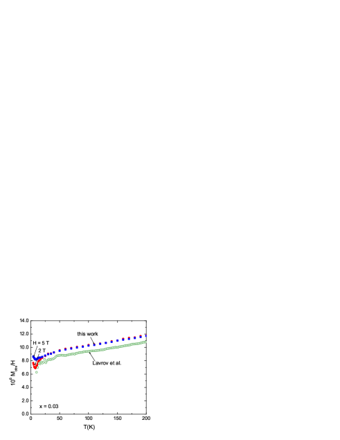
Figure 2: Comparison of the total $M_{obs}/H$ measured at $H$ = 2 and 5 T in sample 03 with the susceptibility anisotropy $\Delta\chi$ inferred from the bulk measurements of Lavrov et al. Ando . In the latter, $\Delta\chi$ is defined as $\chi_{c}-\chi_{ab}$ where the in-plane susceptibility $\chi_{ab}=\frac{1}{2}(\chi_{a}+\chi_{b})$. The results of Lavrov et al.were measured by SQUID magnetometry on a crystal with $x$ = 0.03 (and $\sim$10 times larger than 03 in volume) at the fixed field $H$ = 5 kOe. Above 40 K, the agreement is quite good (the slight offset may come from absolute calibration of the torque cantilever). Below 40 K, the ratio $M_{obs}/H$ is strongly $H$ dependent because of increased contributions from $M_{d}$ and $\Delta M_{s}$.

As a check, we have compared the “raw” data $M_{obs}/H$ in sample 03 against the SQUID magnetometry measurements of Lavrov et al. Ando (Fig. 2). They have reported detailed measurements of the total bulk susceptibilities $\chi_{a}$, $\chi_{b}$ and $\chi_{c}$ in a very large LSCO crystal ($x$ = 0.03) with a volume $\sim$10 times larger than in our samples. In Fig. 2 we plot the $T$ dependence of the anisotropy $\Delta\chi=\chi_{c}-\frac{1}{2}(\chi_{a}+\chi_{b})$. There is good agreement with our corresponding quantity $M_{obs}/H$ measured at 2 and 5 T above 40 K.

III Magnetization results

In the high-field experiments at the NHMFL, all samples (03–09) were investigated to a peak field of 33 T (using Bitter magnets). Further measurements were done on Sample 06 in the hybrid magnet in the field range 11-45 T. In all samples, the high-field data were supplemented by extensive “low-field” in-house results (up to 14 T), which have improved resolution below $\sim$5 T.

Figure 3 shows the general trend of the “raw” observed magnetization $M_{obs}$ vs. $H$ in Samples 03–07 using the low-field data sets. Above the onset temperature for the appearance of vortex-Nernst signal $T_{onset}$, ($\sim$ 30, 40, 60 K in samples 04, 05 and 06, respectively), the $H$-linear term $\Delta\chi^{orb}H$ dominates to produce a fan-like pattern. Below $T_{onset}$, the rapid growth of $M_{d}(T,H)$ which is strongly nonlinear in $H$ produces a noticeable downward deviation from the fan pattern. This is strikingly evident in 055, 06 and 07 but is also seen in 03, 04 and 05. When $T$ decreases below $T_{c}$, the samples with $x>x_{c}$ (055, 06 and 07) display a large diamagnetism even in the limit $H\rightarrow 0$. This requires the vortex solid to be stable. In samples with $x<x_{c}$ (03–05), however, the diamagnetic signal does not grow significantly even with cooling to 0.35 K.

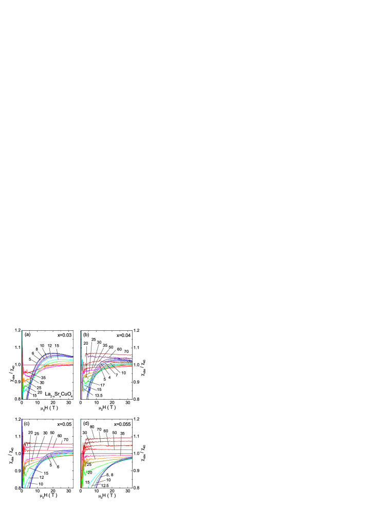
Figure 4: The $H$ dependence of the observed susceptibility $\chi_{obs}\equiv M_{obs}/H$ at selected $T$ in Samples 03, 04, 05 and 055 (Panels a–d, respectively). $\chi_{obs}(T,H)$ is plotted divided by its value at 40 K. In each panel $\chi_{obs}$ is $H$ independent and only weakly $T$ dependent above $\sim$35 K consistent with the van-Vleck term. The strongly $H$-dependent diamagnetic term $M_{d}/H$ grows rapidly between 20 and 5 K. Finally, at low $T$, a third positive contribution – the paramagnetic spin term $\Delta M_{s}/H$ – emerges to counter the diamagnetic term in intense fields. At 5 K, the spin term is barely visible in 055, but quite large in Samples 03 and 04.

Susceptibility The 3 distinct contributions (Eq. 1) to the observed magnetization $M_{obs}$ are actually readily apparent in the raw magnetization data when the field is extended to 33 Tesla. In a linear plot of $M_{obs}$ vs. $H$ (as in Fig. 3a), the terms $M_{d}$ and $\Delta M_{s}$ tend to be dwarfed by the large van-Vleck term $\Delta\chi^{orb}H$, and hard to make out. On the other hand, by simply dividing the raw magnetization by $H$ to form the observed susceptibility $\chi_{obs}\equiv M_{obs}/H$, we can make all 3 terms apparent. Figure 4 shows the field dependence of $\chi_{obs}(T,H)$ in Samples 03–055 at selected $T$ [we display $\chi_{obs}(T,H)$ divided by its curve at 40 K]. First, we look at Panel d (Sample 055). Cooling from 80 K to 35 K, we observe that $\chi_{obs}$ is $H$ independent with a weak $T$ dependence. This high-$T$ behavior of $\chi_{obs}$ leads to the “fan-like” pattern identified with the van-Vleck magnetization $\Delta\chi^{orb}H$ in Fig. 3. The negative contribution of $M_{d}/H$, first resolved near 50 K, grows rapidly in magnitude as $T$ decreases to 5 K. Moreover, while $M_{d}/H$ is very large in low fields, it is suppressed when $H$ exceeds 33 T, consistent with field suppression of the pair condensate. Sample 05 in Panel c shows a similar pattern of behavior except that, below 10 K, a new positive, strongly $H$-dependent contribution emerges to lift the curves upwards (compare curves at 5 and 10 K). Proceeding to Samples 04 and 03 (Panels b and a, respectively), we see that the new paramagnetic term becomes steadily larger with deceasing $x$. This term – associated with the spin contribution $\Delta M_{s}/H$ – is clearly distinguishable from the van-Vleck and diamagnetic terms. In spite of the large spin term in 03 and 04, the diamagnetic term $M_{d}/H$ remains quite robust up to fields of 20-30 T.

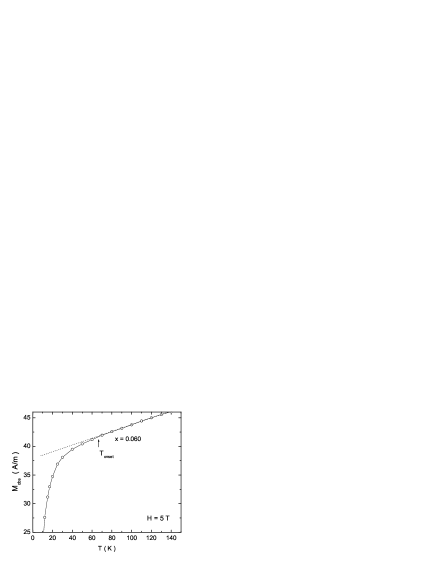
Figure 5: The $T$ dependence of the total observed torque magnetization $M_{obs}$ measured at $H$ = 5 T in sample 06 showing the weak $T$-linear change above $T_{onset}$ (arrows), the onset temperature of diamagnetism. The linear extrapolation (dotted lines) below $T_{onset}$ is used to determine the anisotropic van Vleck contribution $\Delta\chi^{orb}H$. Below $T_{onset}$, the magnitude $|M_{d}|$ increases rapidly.

Removal of van Vleck term As explained in the main text Li06 , it is best to subtract altogether the large “background” van Vleck term $\Delta\chi^{orb}$ to analyze the diamagnetic and spin terms accurately. The broad interval of $T$ in the low-field data set allows $\Delta\chi^{orb}(T)$ to be measured accurately. As an example, Fig. 5 displays the $T$ dependence of $M_{obs}$ (measured at 5 T) in sample 06. When $T>$ 50 K, $M_{obs}$ is dominated by $\Delta\chi^{orb}H$ which has the weak $T$-linear dependence

$$\Delta\chi^{orb}(T)=A\left(1+\frac{T}{T_{0}}\right)$$ (2)

with $A\sim$ 1.05$\times 10^{-5}$ and $T_{0}\sim$ 700 K (dashed line). The temperature scale $T_{0}$ is independent of $x$ to our resolution, while the intercept parameter $A$ shows a very weak $x$ dependence (both are associated with the van Vleck background). However, $T_{onset}$ decreases significantly, nominally linearly with $x$, as $x$ falls below 0.07. The change between 0 and 40 K of this background term is $<6\%$. Using Eq. 2, we remove the van Vleck term to obtain the curves of $M_{orb}^{\prime}(T,H)$, as explained in Ref. Li06 .

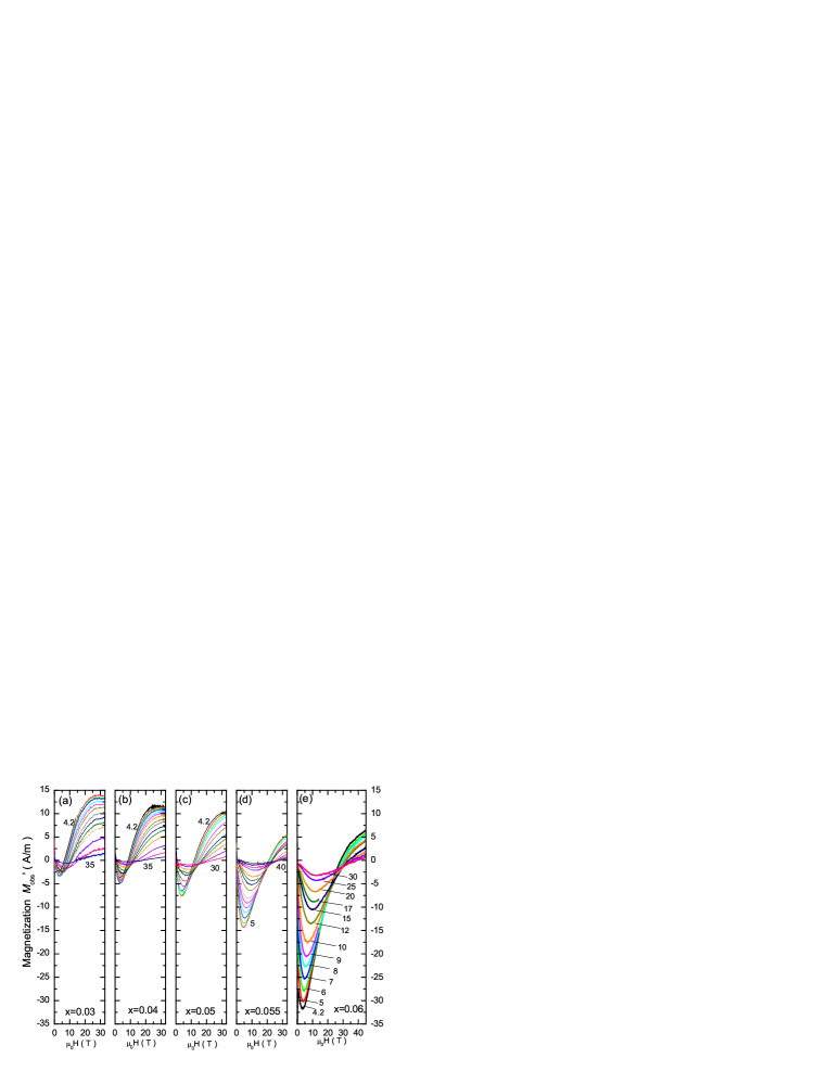
Figure 6: The curves of $M_{orb}^{\prime}$ (observed magnetization with van Vleck term removed) in samples 03, 04, 05, 055 and 06 (Panels a, b, c, d and e, respectively). Each of these curves is comprised of a diamagnetic term $M_{d}(T,H)$ that is dominant in low $H$ ($<$10 T), but is suppressed above 20-30 T, and a paramagnetic spin term $\Delta M_{s}(T,H)$ that is nearly constant in $H$ in high fields. As we increase $x$, the diamagnetic term $M_{d}$ becomes increasingly dominant and harder to suppress in high fields (note expanded field scale in Panel d). Samples 055 and 06 show broad Meissner transitions with $T_{c}\sim$ 0.5 and 5 K, respectively. The other samples show no Meissner transitions. For clarity, we have not displayed curves at $T$ below 4 K (see Fig. 2 in Li06 ).

As anticipated in Fig. 4, the background-subtracted curves $M_{orb}^{\prime}$ reveal an interesting competition between the diamagnetic term $M_{d}(T,H)$ and the spin term $\Delta M_{s}(T,H)$ as $x$ changes from 0.03 to 0.06 (Fig. 6). In sample 03, $M_{d}$ though small is still strong enough to pull $M_{obs}^{\prime}$ negative below $\sim$10 T. Above 10 T, $M_{d}$ is rapidly suppressed to zero at 24 T, leaving the spin term which is nominally $H$ independent. Turning to Panel d for sample 06, we see the same competition between the 2 terms, except that $M_{d}$ is now much larger, and a larger depairing field ($\sim$48 T) is needed to suppress it to zero. Also the saturation value of $\Delta M_{s}$ is only $\frac{1}{2}$ as large. The behaviors in 04, 05 and 055 are intermediate between these 2 extremes.

Paramagnetic spin-$\frac{1}{2}$ moments The overall behavior of the spin term in high fields, together with the oscillatory behavior in weak $H$ (see Fig. 1c of Ref. Li06 ) suggests that the spin term arises from spin-$\frac{1}{2}$ local moments that are nearly non-interacting but have anisotropic $g$-factors ($g_{ab}<g_{c}$) that are weakly $T$-dependent. As derived in Sec. IV, the spin contribution to $M_{obs}$ is

$$\Delta M_{s}(T,H)={\cal P}(T)\tanh[\beta g_{\phi}\mu_{B}B/2],$$ (3)

with $\mu_{B}$ the Bohr magneton and $\beta=1/k_{B}T$. The prefactor is ($N_{s}$ is the spin population)

$${\cal P}(T)=\frac{N_{s}\mu_{B}}{V}\frac{(g_{c}^{2}-g_{ab}^{2})}{2g_{\phi}}\cos\phi.$$ (4)

with the effective $g$-factor

$$g_{\phi}=\sqrt{(g_{c}\cos\phi)^{2}+(g_{ab}\sin\phi)^{2}}.$$ (5)

With $g_{\phi}\sim g_{c}$ fixed at 2.1, the only adjustable parameter at each $T$ is ${\cal P}$.

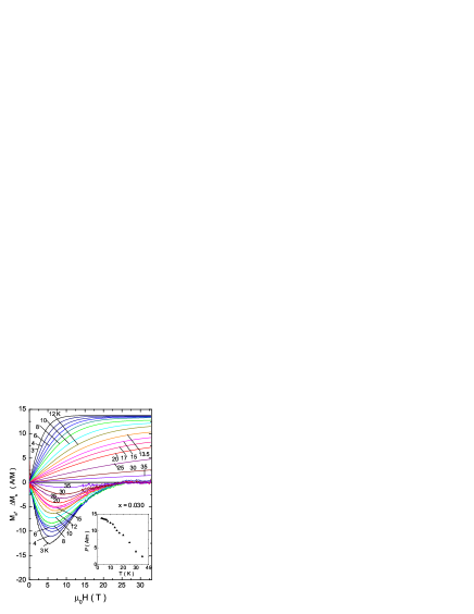
Figure 7: Curves of the the diamagnetic term $M_{d}(T,H)$ and the paramagnetic spin term $\Delta M_{s}(T,H)$ in sample 03 ($x$ = 0.03) at fixed $T$ as indicated. At each $T$, after removing the orbital van-Vleck term, the remaining signal is given by $M_{obs}^{\prime}(T,H)=\Delta M_{s}(T,H)+M_{d}(T,H)$. The plotted curves of $M_{d}$ and $\Delta M_{s}$ add to reproduce $M_{obs}^{\prime}$. The inset shows the $T$ dependence of the prefactor ${\cal P}(T)$ obtained from the fit to Eq. 3.

Using Eq. 3, we may subtract the contribution of the spin term from $M_{obs}^{\prime}$ to obtain the diamagnetic term $M_{d}$ at each $T$. The curves of both $\Delta M_{s}$ and $M_{d}$ in sample 03 are displayed in Fig. 7. The profile of $M_{d}$ resembles the “tilted-hill” profile observed for the vortex-Nernst signal observed at $T>T_{c}$ in both underdoped LSCO (at large doping) and in Bi-based cuprates. The curves here are all associated with the vortex liquid (the vortex solid is not observed in 03 down to 0.35 K).

We remark that the diamagnetic term $M_{d}$ is readily apparent in the raw data of $\chi_{obs}$ vs. $H$ in all samples. Moreover, it remains robust up to high fields of 25-45 T (Fig. 4), so the evidence for the vortex-liquid diamagnetism in samples 03–06 does not depend on our background subtraction or the form of Eq. 3. The merit of Eq. 3 is that it allows us to understand the details of the low-$T$ oscillatory behavior of $M_{obs}^{\prime}$ shown in Fig. 1c of Ref. Li06 , and to extract $M_{d}(T,H)$ with good accuracy.

In Fig. 7, the paramagnetic curves are the best fits using Eq. 3 with the sole adjustable parameter ${\cal P}(T)$ which is plotted in the inset. Below $T_{sg}\sim$ 2.5 K in this sample, the curves of $M_{obs}^{\prime}$ vs. $H$ become slightly hysteretic reflecting the onset of spin-glass behavior. The spin-glass hysteresis loops are clockwise in contrast with the anti-clockwise sense of the loops in the vortex solid (we will discuss the spin-glass observations elsewhere).

IV Anisotropic spin term

The Hamiltonian for an $s=\frac{1}{2}$ spin with anisotropic $g$-factor in a field $\bf B$ (lying in the $x$-$z$ plane at an angle $\phi$ to $\bf z||c$) is

$$H=-\frac{1}{2}\mu_{B}B(g_{ab}\sigma_{x}\sin\phi+g_{c}\sigma_{z}\cos\phi),$$ (6)

where $\sigma_{x}$ and $\sigma_{z}$ are the Pauli matrices and $B={\bf|B|}$. Because of the anisotropy, the tilt-angle $\theta$ of $\vec{\sigma}$ differs from $\phi$. The eigen-spinors of Eq. 6 are

$$|+\rangle=\left(\begin{array}[]{c}\cos\frac{\theta}{2}\\ \sin\frac{\theta}{2}\end{array}\right),\quad\quad|-\rangle=\left(\begin{array}[]{c}-\sin\frac{\theta}{2}\\ \cos\frac{\theta}{2}\end{array}\right)$$ (7)

with $\theta$ defined by

$$\cos\theta=\frac{g_{c}}{g_{\phi}}\cos\phi,\quad\sin\theta=\frac{g_{ab}}{g_{\phi}}\sin\phi,$$ (8)

and $g_{\phi}$ as given in Eq. 5. With Eq. 7, the matrix elements are $\langle+|\sigma_{z}|+\rangle=\cos\theta$ and $\langle+|\sigma_{x}|+\rangle=\sin\theta$ etc.

For a collection of $N_{s}$ spins in a volume $V$ in a bath at temperature $T$, the thermal-averaged magnetization is

$$\langle{\bf M}_{s}\rangle=\frac{N_{s}\mu_{B}}{2V}[g_{c}\cos\theta{\bf\hat{z}}+g_{ab}\sin\theta{\bf\hat{x}}]\tanh[\beta g_{\phi}\mu_{B}B/2].$$ (9)

This contributes the torque signal

$$\tau_{s}=N_{s}\mu_{B}\frac{(g_{c}^{2}-g_{ab}^{2})}{2g_{\phi}}B\cos\phi\sin\phi\tanh[\beta g_{\phi}\mu_{B}B/2],$$ (10)

from which we obtain the results in Eqs. 3–5.

V Hysteretic curves and vortex avalanches

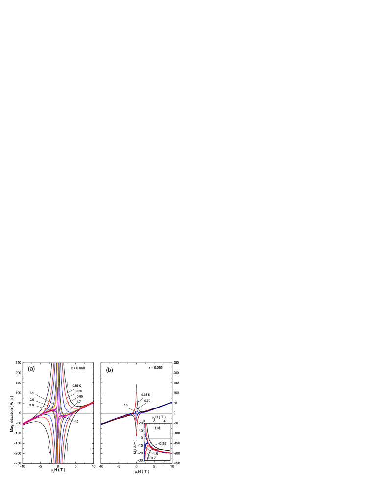
Figure 8: Comparison of the hysteretic loops in Samples 06 (Panel a) and 055 (b). In spite of the small difference in $x$, the hysteresis loops are much larger in 06 than in 055 measured at the same $T$. This reflects the rapid decrease of the zero-Kelvin irreversibility field $H_{irr}(0)$ as $x$ approaches $x_{c}\sim$ 0.055. The inset (Panel c) shows an expanded view of the hysteresis at 0.35, 0.7 and 1.5 K in Sample 055.

A way to see the rapid suppression of the vortex solid state as $x\rightarrow x_{c}^{+}$ is to compare the hysteretic curves of Samples 06 and 055 at low temperatures (Fig. 8). In going from 06 to 055 at $T$ = 0.35 K, the width of the hysteretic loops at a fixed field ($H$ = 1 T) shrinks by $\sim$100. Between 07 and 06, the loops shrink by another factor of 10 (see Fig. 3). The 1000-fold decrease between 07 and 055 provides evidence for a critical transition at $x_{c}$. The opposing view of a distribution of superconducting islands implies a gradual decrease of the hysteretic loops that is inconsistent with our observations.

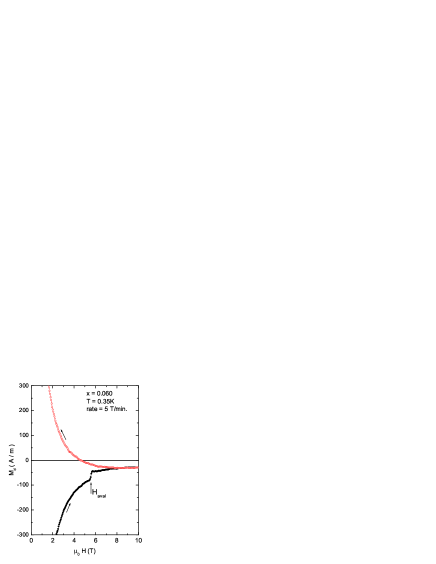
Figure 9: Jumps in the field sweep-up portion of the hysteretic curves of $M_{d}$ vs. $H$ (arrow at $H_{aval}$) in sample 06 at $T$ = 0.35 K at a field sweep rate of 5 T/min. The jumps are not observed when the sweep rates are reduced by a factor of 10. Vortex avalanches are observed only in the vortex-solid phase.

At $T$ = 0.35 K, vortex avalanches can be triggered in the vortex solid ($H<H_{irr}(T)$) by sweeping the field at a rate of 3–5 T/min. As shown in Fig. 9, the jumps occur during the field sweep-up portion of the hysteretic loops. By decreasing the sweep rate by a factor of 10, we can eliminate the jumps altogether. Vortex avalanches occur when the field sweep is too rapid to allow the inserted vortices to equilibrate in the solid phase. They involve collective depinning of a large fraction of the vortices in the crystal in a very short time interval, and are generally considered to be direct evidence for the existence of the vortex solid.

The research at Princeton was supported by the National Science Foundation (NSF) through a MRSEC grant DMR 0213706. Research at CRIEPI was supported by a Grant-in-Aid for Science from the Japan Society for the Promotion of Science. The high field measurements were performed in the National High Magnetic Field Lab. Tallahassee, which is supported by NSF, the Department of Energy and the State of Florida.

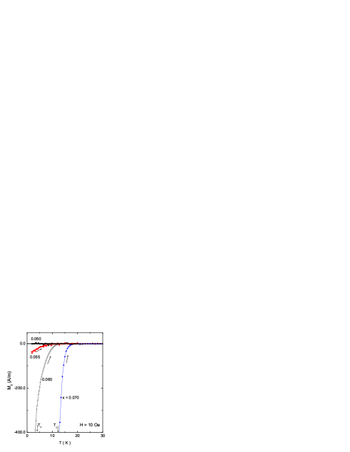
Figure 1: The Meissner curves measured in weak field ($H$= 10 Oe) in samples 05, 055, 06 and 07 measured after zero-field cooling. The Meissner transitions are observed with mid-point temperature $T_{c}$ = 0, 0.5, 5, and 12 K in 05, 055, 06 and 07, respectively. Full flux expulsion (with demagnetization factor $N_{c}\sim$ 2.2) corresponds to $M_{d}$ = -1,900 A/m. It is instructive to compare these ZFC curves with the high-field curves in Fig. 3, which are all in the reversible regime (except below 5 K in 07).

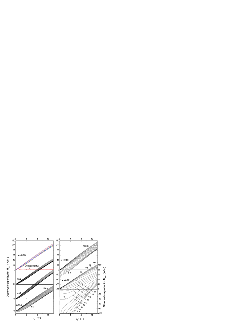
Figure 3: The total (observed) magnetization $M_{obs}$ in the 6 LSCO crystals 03, 04, 05, 055, 06 and 07 with doping $x$ = 0.03, 0.04, 0.05, 0.055, 0.06 and 0.07, respectively. The Meissner transition midpoint $T_{c}\sim$ 0.5, 5 and 12 K in 055, 06 and 07. The range of $T$ in each sample (4-100 K) are similar to the ones indicated for sample 07. All curves share the same scales for the $M_{obs}$ and $H$ axes, but the origins have been shifted vertically for clarity. The background paramagnetic term $\Delta\chi^{orb}H$ is strictly $H$-linear and weakly $T$ dependent (nominally the same in all samples). Below 30 K, the growth of the diamagnetic term $M_{d}$, and the spin anisotropy $\Delta M_{s}$, become increasing evident from 03 to 07. The horizontal bold curve plotted with sample 03 shows the signal of the unloaded cantilever amplified by 10. All curves are in the reversible regime, except in sample 07 where hysteresis appears below 5 K. See Ref. Li06 for discussion of irreversibility.

References

- (1) Lu Li et al., “Low temperature vortex liquid in ”, preprint 2006.
- (2) Yayu Wang et al., Phys. Rev. Lett. 95, 247002 (2005).
- (3) Lu Li et al., Europhys. Lett. 72, 451-457 (2005).
- (4) Seiki Komiya, Yoichi Ando, X. F. Sun, and A. N. Lavrov, Phys. Rev. B 65, 214535 (2002).
- (5) D. E. Farrell et al., Phys. Rev. Lett. 61, 2805-2808 (1988).
- (6) C. Bergemann et al., Phys. Rev. B 57, 14387 (1998).
- (7) A. N. Lavrov, Yoichi Ando, Seiki Komiya, and I. Tsukada, Phys. Rev. Lett. 87, 017007 (2001).