Peltier effect in Andreev interferometers

Abstract

The superconducting proximity effect is known to modify transport properties of hybrid normal–superconducting structures. In addition to changing electrical and thermal transport separately, it alters the thermoelectric effects. Changes to one off-diagonal element $L_{12}$ of the thermoelectric matrix $L$ have previously been studied via the thermopower, but the remaining coefficient $L_{21}$ which is responsible for the Peltier effect has received less attention. We discuss symmetry relations between $L_{21}$ and $L_{12}$ in addition to the Onsager reciprocity, and calculate Peltier coefficients for a specific structure. Similarly as for the thermopower, for finite phase differences of the superconducting order parameter, the proximity effect creates a Peltier effect significantly larger than the one present in purely normal-metal structures. This results from the fact that a nonequilibrium supercurrent carries energy.

In large metallic structures, linear-response transport can be described using the thermoelectric matrix $L$ that relates charge and energy currents to temperature and potential biases. Callen (1948) The off-diagonal coefficients describe coupling between heat and charge currents, and indicate the magnitude of the thermopower and the Peltier effect. In many cases, these coefficients are coupled by Onsager’s reciprocal relation $L_{\alpha\beta}(B)=L_{\beta\alpha}(-B)$ under the reversal of the magnetic field $B$. Onsager (1931); Callen (1948)

In hybrid normal–superconducting systems (see Fig. 1) the Cooper pair amplitude penetrates to the normal-metal parts. This makes the linear-response coefficients $L$ different from their normal-state values, and allows supercurrents $I_{S,\mathrm{eq}}$ to flow through the normal metal even at equilibrium. The charge and energy (entropy) currents $I_{c}^{i}$ and $I_{E}^{i}$ entering different terminals can in linear response be written as

$$\begin{pmatrix}I_{c}^{i}-I_{S,\mathrm{eq}}^{i}\\ I_{E}^{i}\end{pmatrix}=\sum_{j\in\mathrm{terminals}}\begin{pmatrix}L_{11}^{ij}&L_{12}^{ij}\\ L_{21}^{ij}&L_{22}^{ij}\end{pmatrix}\begin{pmatrix}\Delta V_{j}\\ \Delta T_{j}/\bar{T}\end{pmatrix}\,,$$ (1)

in terms of the biases $\Delta{}V_{j}=V_{j}-\bar{V}$, $\Delta{}T_{j}=T_{j}-\bar{T}$ and the modified response coefficients $L$. The proximity-induced changes in the conductance $L_{11}^{ij}$, Charlat et al. (1996); Claughton and Lambert (1996) thermal conductance $L_{22}^{ij}/\bar{T}$ (for $L_{12}^{ij}=L_{21}^{ij}=0$) Claughton and Lambert (1996); Bezuglyi and Vinokur (2003); Jiang and Chandrasekhar (2005a); Jiang and Chandrasekhar (2005b) and thermopower $-L_{12}^{ij}/(\bar{T}L_{11}^{ij})$ Claughton and Lambert (1996); Eom et al. (1998); Seviour and Volkov (2000); Kogan et al. (2002); Parsons et al. (2003a, b); Virtanen and Heikkilä (2004a, b); Jiang and Chandrasekhar (2005c); Volkov and Pavlovskii (2005); Giazotto et al. (2006) have recently been investigated both experimentally and theoretically. Behavior of the remaining off-diagonal coefficient $L_{21}^{ij}$ has previously been discussed in Ref. Claughton and Lambert, 1996 using scattering theory, but the simulations were restricted to small structures — making the contribution from electron-hole asymmetry very large.

In this article, we note that within reasonable approximations, in diffusive superconducting heterostructures Eq. (1) can be generalized to the non-linear regime by defining an energy-dependent thermoelectric matrix $\tilde{L}_{\alpha\beta}^{ij}(E)$. We show that this quantity satisfies an Onsager reciprocal relation $\tilde{L}_{\alpha\beta}^{ij}(E,B)=\tilde{L}_{\beta\alpha}^{ji}(E,-B)$ under the reversal of the magnetic field $B$ and the phase $\arg\Delta$ of the superconducting order parameter, whenever $i$ and $j$ refer to normal terminals. We also show how the proximity effect modifies $L_{21}$ giving rise to a large Peltier effect, Callen (1948) and discuss how it could be experimentally detected.

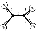
Figure 1: Example of a 4-probe structure considered in the text: 5 normal-metal wires connected to each other and to 4 terminals, of which two are superconducting (S) and two normal (N). We take the lengths $l$, cross-sectional areas $A$, and conductivities $\sigma$ of the wires to be $l/l_{0}=(1.5,1,1.2,1,0.8)$ and $A\sigma/A_{0}\sigma_{0}=(0.8,1,0.8,1,1)$. Here $l_{0}$, $A_{0}$ and $\sigma_{0}$ are some characteristic values, controlling the energy scale $E_{T}=\hbar D/(l_{3}+l_{4}+l_{5})^{2}$ of the proximity effect. The system is chosen so as to bring out effects that depend on the magnitude of geometrical asymmetry. In the numerics, all wires are assumed to be quasi-one-dimensional, $l\gg\sqrt{A}$.

Qualitatively, one can understand the origin of proximity-induced thermoelectric effects by noting that charge current consists of a quasiparticle component and a supercurrent component. That the latter is strongly temperature dependent in proximity structures then leads to a finite $L_{12}$ coefficient, Seviour and Volkov (2000); Virtanen and Heikkilä (2004a) via a mechanism analogous to charge imbalance generation in superconductors. Schmid and Schön (1979); Pethick and Smith (1979) Assuming Onsager symmetry, one would also expect that $L_{21}$ is finite. The actual form of the coupling can be seen by inspecting the quasiclassical transport equations (Eqs. (4) below), or by studying their near-equilibrium approximation in a diffusive normal metal under the influence of a weak proximity effect (see for example Ref. Virtanen and Heikkilä, 2004b):

$$\nabla\cdot J_{c} =0\,,\quad\nabla\cdot J_{E}=0\,,$$ (2a)

$$J_{c} =-\tilde{\sigma}\nabla\delta V+\tilde{\cal T}\nabla\delta T+\frac{\partial J_{S,\rm eq}}{\partial T}\delta T+J_{S,\rm eq}\,,$$ (2b)

$$J_{E} =-\tilde{\sigma}_{\rm th}\nabla\delta T-\bar{T}\tilde{\cal T}\nabla\delta V+\bar{T}\frac{\partial J_{S,\rm eq}}{\partial T}\delta V\,.$$ (2c)

Here, $\delta V$ and $\delta T$ are deviations of the (effective) local potential and temperature from equilibrium, and $\bar{T}$ is the ambient temperature. The first terms in charge and energy current densities $J_{c}$, $J_{E}$ can be considered the quasiparticle current and the rest the (non-equilibrium) supercurrent; $\tilde{\sigma}$ and $\tilde{\sigma}_{\rm th}$ are the proximity-modified charge and thermal conductivities, $J_{S,\rm eq}$ is the equilibrium supercurrent density, and $\tilde{\cal T}$ is a small factor associated with non-equilibrium supercurrent. Although Eqs. (2) are not of the usual form of normal-state transport equations, Callen (1948) one can see that a variation $\delta T$ generates a change in the charge current, and that non-equilibrium ($\delta{}V\neq 0$) supercurrent carries energy current. The corresponding response coefficients in Eqs. (2b) and (2c) are not independent, which is a signature of the Onsager symmetry. Comparing the magnitude of the coefficients, it turns out that at low temperatures a large part of the thermoelectric coupling indeed arises from the temperature-dependence of $J_{S,\rm{}eq}$. At high temperatures where it vanishes exponentially, other sources become more important. Volkov and Pavlovskii (2005); Kogan et al. (2002); Virtanen and Heikkilä (2004b)

However, validity of Eqs. (2) is somewhat restricted, since they are correct only in the linear response and to the first order in the proximity corrections, additionally assuming that the energy gap $\left\lvert{\Delta}\right\rvert$ of the nearby superconductors satisfies $k_{B}\bar{T}\ll\left\lvert{\Delta}\right\rvert$. For quantitative calculations of the multiterminal transport coefficients, and to evaluate the proximity-corrected coefficients in Eq. (2), we start from the full non-equilibrium formalism.

The superconducting proximity effect can be described using the quasiclassical BCS–Gor’kov theory. Kopnin (2001); Belzig et al. (1999) Here, we concentrate on diffusive normal-metal structures that are connected to superconducting and normal terminals, and neglect any inelastic scattering. The model then reduces to the Usadel equations, Usadel (1970); Belzig et al. (1999) whose first part, the spectral equations, can in this case be written as

$$D\nabla^{2}\theta=-2i(E+i0^{+})\sinh\theta+\frac{v_{S}^{2}}{2D}\sinh(2\theta)\,,$$ (3a)

$$\nabla\cdot(-v_{S}\sinh^{2}\theta)=0\,,\quad v_{S}\equiv D(\nabla\chi-2e{\bf A}/\hbar)\,.$$ (3b)

They describe the penetration of the superconducting pair amplitude $F=e^{i\chi}\sinh\theta$ into the normal metal. We denote the diffusion constant of the metal here by $D$, and the magnetic vector potential by ${\bf A}$. At clean contacts to bulk superconductors, the pairing angle is $\theta=\operatorname{artanh}(\left\lvert{\Delta}\right\rvert/E)$ and the phase $\chi=\arg\Delta$, where $\Delta$ is the superconducting order parameter. Transport properties are in turn determined by kinetic Boltzmann-like equations

$$D\nabla\cdot\hat{\Gamma}_{T}f={\cal R}f_{T}+D(\nabla\cdot{}j_{S})f_{L},\;D\nabla\cdot\hat{\Gamma}_{L}f=0,$$ (4a)

$$\hat{\Gamma}_{T}f\equiv\mathcal{D}_{T}\nabla f_{T}+\mathcal{T}\nabla f_{L}+j_{S}f_{L}\,,$$ (4b)

$$\hat{\Gamma}_{L}f\equiv\mathcal{D}_{L}\nabla f_{L}-\mathcal{T}\nabla f_{T}+j_{S}f_{T}\,,$$ (4c)

that describe the behavior of the antisymmetric and symmetric parts $f_{L}(E)\equiv{}f(\mu_{S}-E)-f(\mu_{S}+E)$ and $f_{T}(E)\equiv{}1-f(\mu_{S}-E)-f(\mu_{S}+E)$ of the electron distribution function. They are defined with respect to the potential of the superconductors, chosen below as $\mu_{S}=0$. The spectral supercurrent $j_{S}$, the diffusion coefficients $\mathcal{D}_{L}$, $\mathcal{D}_{T}$, $\mathcal{T}$, and the condensate sink term ${\cal R}$ are functionals of $\theta$ and $\chi$, having the symmetries $\mathcal{D}_{L/T}(\chi)=\mathcal{D}_{L/T}(-\chi)$, $\mathcal{T}(\chi)=-\mathcal{T}(-\chi)$, $j_{S}(\chi)=-j_{S}(-\chi)$, ${\cal R}(\chi)={\cal R}(-\chi)$. Belzig et al. (1999); Virtanen and Heikkilä (2004b) In normal metals, $\nabla\cdot{}j_{S}={\cal R}=0$. Observable current densities are finally related to the spectral currents $\hat{\Gamma}_{L/T}f$ through

$$J_{c}=-\frac{\sigma}{2\left\lvert{e}\right\rvert}\int_{-\infty}^{\infty}\mathrm{d}E\,\hat{\Gamma}_{T}f\,,\;J_{E}=\frac{\sigma}{2e^{2}}\int_{-\infty}^{\infty}\mathrm{d}E\,E\,\hat{\Gamma}_{L}f\,.$$ (5)

and the heat current density is $J_{Q}=J_{E}-VJ_{c}$ at the terminals. Below, we also assume that all contacts to terminals are clean and of negligible resistance: in this case all quantities are continuous at the interfaces, except at superconductors for $E<\left\lvert{\Delta}\right\rvert$ the boundary condition for the kinetic L-mode is changed to $\hat{\mathbf{n}}\cdot\hat{\Gamma}_{L}f=0$, where $\hat{\mathbf{n}}$ is the normal to the interface.

It is important to note that the last two terms in Eqs. (4) mix the L and T modes and cause thermoelectric effects: near equilibrium, they lead to the coupling terms in Eqs. (2). Away from linear response, a non-equilibrium modification of the distribution function $f$ due to the mixing Heikkilä et al. (2003) has also been experimentally observed in Ref. Crosser et al., 2006.

The aim in the following is to calculate the thermoelectric coefficients $L_{\alpha\beta}^{ij}$ starting from Eqs. (4). However, as with the charge conductance, it is useful to first define corresponding energy-dependent thermoelectric coefficients $\tilde{L}_{\alpha\beta}^{ij}(E)$. Since the kinetic equations are linear, it is possible to write the currents entering different terminals as

$$I_{c}^{i} =\int_{-\infty}^{\infty}\mathrm{d}E\,\,\sum_{\beta j}\tilde{L}_{T\beta}^{ij}(E)f_{\beta}^{j}(E)\,,$$ (6a)

$$I_{E}^{i} =\int_{-\infty}^{\infty}\mathrm{d}E\,\,E\,\sum_{\beta j}\tilde{L}_{L\beta}^{ij}(E)f_{\beta}^{j}(E)\,,$$ (6b)

where $\beta\in\{T,L\}$, $j$ runs over all terminals, and $f_{\alpha}^{j}$ is the $\alpha$-mode distribution function in terminal $j$. This spectral thermoelectric matrix $\tilde{L}_{\alpha\beta}^{ij}(E)$ is the quasiclassical counterpart to the $P$-matrix in Ref. Claughton and Lambert, 1996. More explicitly, $\tilde{L}_{\alpha\beta}^{ij}(E)$ can be defined as the $\alpha$-mode current seen in terminal $i$ that a unit excitation of mode $\beta$ in terminal $j$ generates at energy $E$:

$$\tilde{L}^{ij}_{\alpha\beta}(E)\equiv\int_{\mathcal{S}_{i}}\mathrm{d}\mathcal{S}\,\,\hat{\mathbf{n}}\cdot\hat{\Gamma}_{\alpha}\psi^{j,\beta}\,.$$ (7)

Here, $\mathcal{S}_{i}$ is the surface of terminal $i$ and $\hat{\mathbf{n}}$ the corresponding normal vector. The two-component function $\psi^{j\beta}$ is assumed to satisfy the kinetic equations (4) with the electron distribution functions $f_{\alpha}^{i}$ in terminals replaced by $\delta_{\alpha\beta}\delta_{ij}$. The linear-response coefficients $L$ are directly related to $\tilde{L}(E)$ via Eq. (6), for example $L_{11}=\frac{1}{2k_{B}T}\int\mathrm{d}E\,\tilde{L}_{TT}(E)\operatorname{sech}^{2}(\frac{E}{2k_{B}T})$ and $L_{21}=\frac{-1}{2k_{B}T}\int\mathrm{d}E\,E\,\tilde{L}_{LT}(E)\operatorname{sech}^{2}(\frac{E}{2k_{B}T})$.

The spectral thermoelectric matrix depends only on $\theta$ and $\chi$, but not on the distribution functions at the terminals. Knowing the energy dependence of this matrix, one can directly evaluate currents also away from linear response, if changes in the order parameter $\Delta$ and any inelastic scattering can be neglected. The matrix $\tilde{L}_{\alpha\beta}^{ij}(E)$ one can evaluate numerically once $\theta$ and $\chi$ have been solved, and it offers a feasible way to find the response of the circuit to different types of excitations in the terminals.

An Onsager reciprocal relation for $\tilde{L}_{\alpha\beta}^{ij}(E)$ follows from the fact that the differential operator $\hat{\mathcal{L}}$ in Eqs. (4), $\hat{\mathcal{L}}f=0$, has the property

$$\hat{\mathcal{L}}(B)^{\dagger} =(-\nabla)\cdot\begin{pmatrix}\mathcal{D}_{T}&\mathcal{T}\\ -\mathcal{T}&\mathcal{D}_{L}\end{pmatrix}^{\dagger}(-\nabla)+(-\nabla)\cdot\begin{pmatrix}0&j_{S}\\ j_{S}&0\end{pmatrix}^{\dagger}$$ (8)

$$\quad-\begin{pmatrix}{\cal R}&-D(\nabla\cdot{}j_{S})\\ 0&0\end{pmatrix}$$

$$=\hat{\mathcal{L}}(-B)\,,$$

due to the symmetries of the coefficients under reversal of the phases $\chi$, $\arg\Delta$ and the magnetic field $B$. Below, whenever we discuss reversal of $B$, also reversal of the phases is implied. Integration by parts now shows that for any volume $\Omega$ and two-component functions $\phi$, $\psi$, we can write

$$\int_{\Omega}\mathrm{d}\mathcal{V}\,[\psi^{\dagger}\hat{\mathcal{L}}\phi-\phi^{\dagger}\hat{\mathcal{L}}^{\dagger}\psi]=\int_{\partial\Omega}\mathrm{d}\mathcal{S}\,\hat{\mathbf{n}}\cdot J\,,$$ (9)

where $\partial\Omega$ is the boundary of $\Omega$. For the differential operator here, the flux $J=\psi^{\dagger}\hat{\Gamma}(B)\phi-\phi^{\dagger}\hat{\Gamma}(-B)\psi-j_{S}\psi^{\dagger}\sigma_{1}\phi$, $\sigma_{1}$ being the first spin matrix. Now, we choose $\Omega$ to be the whole conductor, with $\phi$ and $\psi$ such that $\phi=\psi^{j,\beta}$ satisfies the conditions in the calculation for $\tilde{L}_{\alpha\beta}^{ij}(E,B)$ and $\psi=\psi^{i,\alpha}$ the conditions for $\tilde{L}_{\beta\alpha}^{ji}(E,-B)$. When both $i$ and $j$ refer to normal terminals, we then find

$$\begin{split}0&=\int_{\partial\Omega}\mathrm{d}\mathcal{S}\,\hat{\mathbf{n}}\cdot J\\ &=\int_{\mathcal{S}_{i}}\mathrm{d}\mathcal{S}\,\hat{\mathbf{n}}\cdot\hat{\Gamma}_{\alpha}(B)\phi-\int_{\mathcal{S}_{j}}\mathrm{d}\mathcal{S}\,\hat{\mathbf{n}}\cdot\hat{\Gamma}_{\beta}(-B)\psi\,,\end{split}$$ (10)

using the boundary conditions imposed on $\phi$ and $\psi$, and the fact that $j_{S}=0$ at normal terminals. Comparison of Eqs. (10) and (7) reveals a reciprocal relation

$$\tilde{L}_{\alpha\beta}^{ij}(E,B)=\tilde{L}_{\beta\alpha}^{ji}(E,-B)\,.$$ (11)

This implies that phase differences in the order parameter will be similar sources for quasiclassical Peltier and Thompson effects as they are for the thermopower discussed in Refs. Seviour and Volkov, 2000; Kogan et al., 2002; Virtanen and Heikkilä, 2004a, b; Volkov and Pavlovskii, 2005. Similar relations exist also in the scattering theory. Claughton and Lambert (1996)

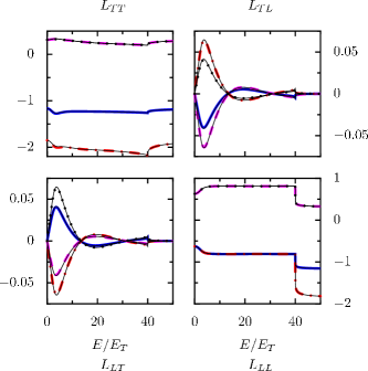
Figure 2: (Color online) Elements $L^{ij}_{\alpha\beta}$ for $i,j=1,2$ and $\alpha,\beta=L,T$ for the asymmetric interferometer in Fig. 1, in units of $1/R_{2}$. The order parameters in the superconducting terminals have $\arg\Delta_{3}-\arg\Delta_{4}=0.54\pi$ and $\left\lvert{\Delta_{3}}\right\rvert=\left\lvert{\Delta_{4}}\right\rvert=40E_{T}$. Thick blue solid line is $L^{11}$, dash-dotted red line $L^{22}$, black dotted line $L^{12}$ and magenta dashed line $L^{21}$. Note the symmetry $\tilde{L}_{\alpha\beta}^{ij}(E)=(-1)^{1-\delta_{\alpha\beta}}\tilde{L}_{\beta\alpha}^{ji}(E)$. Approximations found by solving Eqs. (4) to first order in $j_{S}$ and $\mathcal{T}$ are shown as thin solid lines — in general they are indistinguishable from the exact numerical results.

The form of Eqs. (6) also implies that $\tilde{L}(E,B)$ has the symmetries

$$\sum_{j}\tilde{L}^{ij}_{TL}(E)=0\qquad\text{for normal terminal $i$,}$$ (12a)

$$\sum_{j}\tilde{L}^{ij}_{LL}(E)=0\,,$$ (12b)

$$\tilde{L}^{ij}_{\alpha\beta}(E,-B)=(-1)^{1-\delta_{\alpha\beta}}\tilde{L}^{ij}_{\alpha\beta}(E,B)\,,$$ (12c)

since the charge current to any normal terminal and the entropy current to any terminal must vanish at equilibrium for all temperatures. Equation (12c) follows essentially from the electron-hole symmetry assumed in the quasiclassical theory, leading to $\hat{\Gamma}_{L}{}f\mapsto{}\hat{\Gamma}_{L}{}f$, $\hat{\Gamma}_{T}{}f\mapsto-\hat{\Gamma}_{T}{}f$ under the transformations $B\mapsto-B$, $f_{T}\mapsto-f_{T}$. Virtanen and Heikkilä (2004b) This makes the diagonal coefficients symmetric in $B$ and the off-diagonal ones antisymmetric. However, there are some experimental results Eom et al. (1998); Jiang and Chandrasekhar (2005c) where the latter symmetry does not hold. Such observations cannot be explained with the quasiclassical theory applied here.

Consider now the application of the formulation above in the structure in Fig. 1. We solve the spectral equations (3) in this structure numerically and calculate the spectral thermoelectric matrix from the solutions. Behavior of the two coefficients important for thermoelectric effects, spectral supercurrent $j_{S}$ and the coefficient $\mathcal{T}$, is discussed for structures of this type for example in Refs. Heikkilä et al., 2002; Virtanen and Heikkilä, 2004b. Resulting elements of $L^{ij}_{\alpha\beta}(E)$ are plotted as a function of $E$ in Fig. 2 — the energy scale is given by the Thouless energy $E_{T}=\hbar D/(l_{3}+l_{4}+l_{5})^{2}$. The diagonal elements $\tilde{L}_{TT}(E)$ and $\tilde{L}_{LL}(E)$ are spectral charge and energy conductances. Charlat et al. (1996); Bezuglyi and Vinokur (2003) At $E>\left\lvert{\Delta}\right\rvert$, energy current can enter also the superconductor, which is visible as a rapid change in the $\tilde{L}_{LL}$-coefficient. The off-diagonal coefficients qualitatively follow the energy dependence of the spectral supercurrent $j_{S}$ which gives the most visible contribution. Moreover, the elements of the matrix clearly exhibit the symmetries (11) and (12).

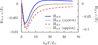
Figure 3: (Color online) Peltier coefficients $\Pi_{NN}$, $\Pi_{NS}$ for the same parameters as in Fig. 2. Approximations (14a), (14b) are shown as thin lines – deviation from the exact result is due to neglecting $\mathcal{T}$.

The finite coefficient $\tilde{L}_{LT}^{ij}(E)$ leads to a Peltier effect: assume that the terminals are at a constant temperature $T^{i}=\bar{T}$ and biased at potentials chosen so that a current $I_{c}$ flows between terminals 1 and 2, $I_{c}^{1}=-I_{c}^{2}=I_{c}$. Then, the Peltier linear-response coefficient for this system is

$$\Pi_{NN}\equiv\frac{dI_{Q}^{1}}{dI_{c}^{1}}=\frac{dI_{E}^{1}}{dI_{c}^{1}}=\frac{L_{21}^{11}W_{1}-L_{21}^{12}W_{2}}{L_{11}^{11}W_{1}-L_{11}^{12}W_{2}}\,,$$ (13)

where $W_{j}\equiv(L_{11}^{1j}+L_{11}^{2j})^{-1}$. We can also define the Peltier coefficient $\Pi_{NS}\equiv\frac{1}{2}dI_{E}^{1}/dI_{c}^{1}$ corresponding to the current configuration $I_{c}^{1}=I_{c}^{2}=I_{c}/2$.

The magnitude and temperature dependence of $\Pi$ is shown in Fig. 3. For a typical Thouless energy of $E_{T}=200\,\mathrm{mK}\,k_{B}$ of an Andreev interferometer, the Peltier coefficients would be $\left\lvert{\Pi_{NN}}\right\rvert\sim 100\,\mathrm{nV}$ and $\left\lvert{\Pi_{NS}}\right\rvert\sim 1\,\mathrm{\mu{}V}$ at $T\sim 200\,\mathrm{mK}$. For comparison, Peltier coefficients for purely normal-metal junctions at these temperatures are of the order $\Pi=T(S^{B}-S^{A})\sim 0.2\,\mathrm{K}\times 10\,\nicefrac{\mathrm{nV}}{\mathrm{K}}=2\,\mathrm{nV}$. The interferometer induces a significantly larger $\Pi$.

The above Peltier effect is related to the thermopower discussed in Refs. Virtanen and Heikkilä, 2004a; Seviour and Volkov, 2000. We indeed find the Kelvin relations $\Pi_{NN}=TS_{NN}$, $\Pi_{NS}=TS_{NS}$, which follow from the Onsager symmetry. Similarly as in Ref. Virtanen and Heikkilä, 2004b, within the assumptions where Eqs. (2) apply, one can also find simple approximations up to first order in $j_{S}$:

$$\Pi_{NN} \approx\frac{(R_{3}-R_{4})R_{5}^{2}}{2(R_{1}+R_{2}+R_{5})(R_{3}+R_{4}+R_{5})}\frac{k_{B}T}{e}\frac{\mathrm{d}I_{S,eq}\,}{\mathrm{d}T\,}\,,$$ (14a)

$$\Pi_{NS} \approx\frac{4R_{3}R_{4}R_{5}+R_{5}^{2}(R_{3}+R_{4})}{4(R_{1}+R_{2}+R_{5})(R_{3}+R_{4}+R_{5})}\frac{k_{B}T}{e}\frac{\mathrm{d}I_{S,eq}\,}{\mathrm{d}T\,}\,.$$ (14b)

Here, $I_{S,eq}\equiv\frac{A\sigma}{2}\int_{-\infty}^{\infty}\mathrm{d}E\,\,j_{S}\tanh\frac{E}{2k_{B}T}$ is the equilibrium supercurrent. The above also shows the dependence on the asymmetry for $\Pi_{NN}$ and the proportionality to the supercurrent — for this contribution to the effect.

Finite Peltier coefficients allow for cooling one of the terminals by driving electric current. Assume the terminal is small enough, such that the power flowing into the phonons is small compared to the heat current carried by electrons. The temperature change is then limited by the Joule heat generated in the wires: the heat current is $I_{Q}^{1}=-G_{th}\Delta T_{1}-2\Pi_{NS}I_{c}^{1}+e(I_{c}^{1})^{2}/G$, $G$ and $G_{th}$ being electrical and heat conductances. The maximum cooling effect then is, in a rough estimate assuming that Wiedemann-Franz law applies, $\Delta T_{1}=-(3/\pi^{2})(e^{2}\Pi_{NS}^{2}/k_{B}T)/k_{B}\sim-0.3\,\mathrm{mK}$ for $E_{T}=200\,\mathrm{mK}k_{B}$. Numerical calculation in the structure of Fig. 1 yields cooling $\Delta{}T\sim-0.4\,\mathrm{mK}$, as shown in Fig. 4.

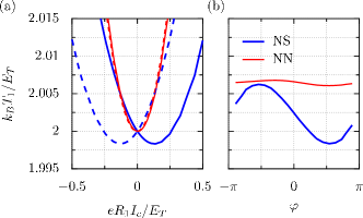
Figure 4: (Color online) Temperature of terminal 1 in Fig. 1 (a) for $\varphi=\arg\Delta_{3}-\arg\Delta_{4}=\pm 0.54\pi$ (dashed and solid lines) and current configurations corresponding to $\Pi_{NN}$ and $\Pi_{NS}$ (red and blue lines), as a function of $I_{c}$. (b) $T_{1}$ for $eR_{1}I_{c}/E_{T}=0.15$, as a function of $\varphi$. The results are calculated assuming other terminals are at the temperature $T=2E_{T}/k_{B}$. Deviation of $T_{1}$ from $T$ originates from Joule heating and the oscillation of the proximity-Peltier effect.

One point to note is that also the $B$-symmetric oscillation of the thermal conductance Bezuglyi and Vinokur (2003); Jiang and Chandrasekhar (2005a) contributes to the temperature change, although this is significant only at temperatures small compared to $E_{T}/k_{B}$. In the absence of the Peltier effect, $\Delta T$ would hence be symmetric in $B$ and always positive. The proximity-Peltier effect allows negative temperature changes and also breaks the symmetry, which makes the antisymmetric part $T_{1}(B)-T_{1}(-B)$ the experimentally interesting signal. In the structure of Fig. 1 the oscillation amplitude can be of the order of 1 mK for $E_{T}=200\,\mathrm{mK}k_{B}$. (See Fig. 4b.) Temperature changes of this order can be experimentally resolved in mesoscopic structures, Meschke et al. (2006) so that the detection of the effect simply via observing $\Delta T$ should be experimentally viable. In addition to the off-diagonal thermoelectric coefficients $L_{12}$, $L_{21}$, it would also be interesting to study the Onsager reciprocity for $\tilde{L}^{ij}_{TT}(E)$ via differential conductances in multi-terminal structures.

In summary, we have studied charge and energy transport and its symmetry relations in normal–superconducting hybrid structures. We show that a large Peltier effect controlled by the phase difference over a Josephson junction can arise, partly due to co-flowing quasiparticle and supercurrents. This complements previous studies of a related effect in the thermopower.

This research was supported by the Finnish Cultural Foundation and the Academy of Finland. We thank M. Meschke and I. A. Sosnin for useful discussions.

References

- Callen (1948) H. B. Callen, Phys. Rev. 73, 1349 (1948).
- Onsager (1931) L. Onsager, Phys. Rev. 37, 405 (1931).
- Charlat et al. (1996) P. Charlat, H. Courtois, Ph. Gandit, D. Mailly, A. F. Volkov, and B. Pannetier, Phys. Rev. Lett. 77, 4950 (1996).
- Claughton and Lambert (1996) N. R. Claughton and C. J. Lambert, Phys. Rev. B 53, 6605 (1996).
- Bezuglyi and Vinokur (2003) E. V. Bezuglyi and V. Vinokur, Phys. Rev. Lett. 91, 137002 (2003).
- Jiang and Chandrasekhar (2005a) Z. Jiang and V. Chandrasekhar, Phys. Rev. Lett. 94, 147002 (2005a).
- Jiang and Chandrasekhar (2005b) Z. Jiang and V. Chandrasekhar, Phys. Rev. B 72, 020502(R) (2005b).
- Eom et al. (1998) J. Eom, C.-J. Chien, and V. Chandrasekhar, Phys. Rev. Lett. 81, 437 (1998).
- Seviour and Volkov (2000) R. Seviour and A. F. Volkov, Phys. Rev. B 62, R6116 (2000).
- Kogan et al. (2002) V. R. Kogan, V. V. Pavlovskii, and A. F. Volkov, Europhys. Lett. 59, 875 (2002).
- Virtanen and Heikkilä (2004a) P. Virtanen and T. T. Heikkilä, Phys. Rev. Lett. 92, 177004 (2004a).
- Virtanen and Heikkilä (2004b) P. Virtanen and T. T. Heikkilä, J. Low Temp. Phys. 136, 401 (2004b).
- Volkov and Pavlovskii (2005) A. F. Volkov and V. V. Pavlovskii, Phys. Rev. B 72, 14529 (2005).
- Jiang and Chandrasekhar (2005c) Z. Jiang and V. Chandrasekhar, Chinese J. Phys. 43, 693 (2005c).
- Parsons et al. (2003a) A. Parsons, I. A. Sosnin, and V. T. Petrashov, Phys. Rev. B 67, 140502(R) (2003a).
- Parsons et al. (2003b) A. Parsons, I. A. Sosnin, and V. T. Petrashov, Physica E 18, 316 (2003b).
- Giazotto et al. (2006) F. Giazotto, T. T. Heikkilä, A. Luukanen, A. Savin, and J. Pekola, Rev. Mod. Phys. 78, 217 (2006).
- Schmid and Schön (1979) A. Schmid and G. Schön, Phys. Rev. Lett. 43, 793 (1979).
- Pethick and Smith (1979) C. J. Pethick and H. Smith, Phys. Rev. Lett. 43, 640 (1979).
- Kopnin (2001) N. B. Kopnin, Theory of nonequilibrium superconductivity, no. 110 in International series of monographs on physics (Oxford University Press, 2001).
- Belzig et al. (1999) W. Belzig, F. K. Wilhelm, C. Bruder, G. Schön, and A. D. Zaikin, Superlatt. Microstruct. 25, 1251 (1999).
- Usadel (1970) K. D. Usadel, Phys. Rev. Lett. 25, 507 (1970).
- Heikkilä et al. (2003) T. T. Heikkilä, T. Vänskä, and F. K. Wilhelm, Phys. Rev. B 67, 100502(R) (2003).
- Crosser et al. (2006) M. S. Crosser, P. Virtanen, T. T. Heikkilä, and N. O. Birge, Phys. Rev. Lett. 96, 167004 (2006).
- Heikkilä et al. (2002) T. T. Heikkilä, J. Särkkä, and F. K. Wilhelm, Phys. Rev. B 66, 184513 (2002).
- Meschke et al. (2006) M. Meschke, W. Guichard, and J. Pekola, Nature 444, 187 (2006).