Exact relaxation in a class of non-equilibrium quantum lattice systems

Abstract

A reasonable physical intuition in the study of interacting quantum systems says that, independent of the initial state, the system will tend to equilibrate. In this work we study a setting where relaxation to a steady state is exact, namely for the Bose-Hubbard model where the system is quenched from a Mott quantum phase to the strong superfluid regime. We find that the evolving state locally relaxes to a steady state with maximum entropy constrained by second moments, maximizing the entanglement, to a state which is different from the thermal state of the new Hamiltonian. Remarkably, in the infinite system limit this relaxation is true for all large times, and no time average is necessary. For large but finite system size we give a time interval for which the system locally “looks relaxed” up to a prescribed error. Our argument includes a central limit theorem for harmonic systems and exploits the finite speed of sound. Additionally, we show that for all periodic initial configurations, reminiscent of charge density waves, the system relaxes locally. We sketch experimentally accessible signatures in optical lattices as well as implications for the foundations of quantum statistical mechanics.

I Introduction

The study of the non-equilibrium properties of quantum many body systems has recently entered a renaissance era. This has been motivated, in part, by recent experimental developments; the rapid progress of experiments involving ultracold atoms in optical lattices, with their high degree of control and long coherence times, has opened the door to precise experimental studies of the dynamics of strongly interacting quantum systems Experiments . In addition, questions of relaxation and thermalisation for non-equilibrium systems are again receiving attention from foundational perspectives. This is partly triggered by intuition from quantum information theory where maximally or almost maximally entangled states emerge from appropriate distributions of random states [2–4].

One particularly fascinating setting which has recently received intensive study is that of quenching, that is, a sudden change of interaction strength [5–12]. Several explanations for, and numerical studies of, quenched dynamics have gradually led to the formulation of a rather general body of theory and conjectures; it has been mooted that if the system starts in the ground state of one Hamiltonian then certain properties such as correlators of the system should relax to an analogue of the thermal state of the new Hamiltonian after a quench [5, 7–9]. Thus we are motivated by these observations to formulate a conjecture. This local relaxation conjecture states that a system should locally relax to a steady state, respecting conserved quantities of motion.

The local relaxation conjecture may sound suspiciously like a violation of unitarity as the global state must, of course, remain pure throughout the dynamics. However, a reasonable physical intuition which explains why there is no contradiction is that for a small block of sites the rest of a system acts like a reservoir and thus allows the site to maximise its entropy subject to the constraint that the energy is preserved. Indeed, the full explanation for the emergence of a local steady state during the course of the quench may be intuitively described along these lines: as time evolves the system becomes correlated Entanglement – from each site a wavefront moving at the speed of sound for the lattice emerges carrying information. As time progresses more and more excitations will have passed through a given site, see Fig. 1. The cumulative effect of these successive excitations results in an effective averaging process; information stored in one site becomes infinitely diluted across the lattice as time progresses. A similar intuition has been recently emphasised by Calabrese and Cardy calabrese in the context of quenching to a critical system.

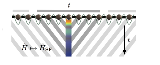
Figure 1: Intuitive picture of the relaxation process in the quenched Bose-Hubbard model as discussed in the main text: For any lattice site $i$ (or any block of sites) within a cone (dark grey) defined by the speed of sound excitations significantly contribute to the local mixing of the state at the site. Contributions from outside this cone (light grey) are exponentially suppressed. The incommensurate influence of the lattice sites in the cone gives rise to a relaxation to maximal entropy for large times $t$. When the excitations have travelled through the entire lattice, recurrences will occur.

In this work we introduce a physical setting where the local relaxation conjecture can be studied analytically. We find an exact convergence of all local states to a steady state for long times in the quenched Bose-Hubbard model. We imagine the system starts in a Mott insulator phase and is then suddenly switched to the deep superfluid regime. Our method is self-contained and physically motivated, and is valid also for finite system sizes relevant to experimental settings. In the course of the proof we are also able to quantify the dilution of information throughout the lattice. Thus, our approach is considerably simpler and more physically intuitive than a potential approach based on the $C^{*}$-algebraic arguments developed in Ref.  Robinsonandfriends to study the local relaxation of free fermions and bosons freely moving in $\mathbb{R}^{n}$ and classical systems Spohn . Interestingly, the convergence is not only true in the time average, but actually true for any large instant of time. This is in contrast to the recent approaches developed in quantum information Brodyandco , where, in order to study this problem, it would seem necessary to consider the time-averaged local state rather than the local state itself. Additionally, our approach does not require the system being quenched to to be critical — we obtain the same results regardless of whether the system being quenched to is critical or not. For blocks of sites we also find a relaxation, but not to the thermal state of the new Hamiltonian.

II Quenched Bose-Hubbard dynamics

We start from a Bose-Hubbard Hamiltonian, modeling, for example, a dilute gas of ultra-cold atoms which are Bose-condensed in an optical lattice Classic . In one dimension (generalizations of our findings to higher dimensions are entirely straightforward) it reads $\hat{H}=\hat{H}_{\text{SF}}+\hat{U}$, where

$$\hat{H}_{\text{SF}}=-J\sum_{\langle i,j\rangle}\hat{b}_{i}^{\dagger}\hat{b}_{j},\;\hat{U}=\frac{U}{2}\sum_{i=1}^{N}\hat{n}_{i}(\hat{n}_{i}-1)-\mu\sum_{i=1}^{N}\hat{n}_{i}.$$ (1)

Here $\hat{b}_{1},\dots,\hat{b}_{N}$ denote the bosonic annihilation operators, and $\hat{n}_{i}=\hat{b}_{i}^{\dagger}\hat{b}_{i}$. The coefficient $J$ is the hopping matrix element, governing the strength of hopping to neighboring sites ($\langle i,j\rangle$ indicates summation over nearest neighbors) and $U$ defines the strength of the on-site interaction. Finally, the chemical potential $\mu$ controls the particle number. For theoretical simplicity we shall assume that that the system is translationally invariant with periodic boundary conditions, so that the underlying lattice is a ring. This Hamiltonian exhibits two distinct phases as $J$ and $U$ are varied. When the hopping dominates, that is $J\gg U$, the system is in a superfluid phase. For a dominant on-site repulsion the ground state is a Mott insulator.

We imagine that the system is initially held at chemical potential $\mu$ and is in the ground state in the Mott regime Classic . In this deep Mott phase (corresponding to $J=0$) the ground state vector is a product $|m\rangle^{\otimes N}$ of individual number state vectors $|m\rangle$ of $m$ bosons at each site. Here, $m=\max\{0,[(\mu/U+1)/2]\}$, where $[\cdot]$ denotes the closest integer to the value in brackets. We then imagine that the system is rapidly quenched, at $t=0$, to the strong superfluid regime $J\gg U$. We model this quench by an instantaneous change in the Hamiltonian to the regime $U=0$. Thus the system state vector at time $t$, $|\psi(N,t)\rangle$, is given by (we set $\hbar=1$)

$$|\psi(N,t)\rangle=\mathrm{e}^{-\mathrm{i}t\hat{H}_{\text{SF}}}|m\rangle^{\otimes N}.$$ (2)

III Relaxation for a single site

As outlined earlier, we are interested in whether subsystems consisting of single sites or blocks thereof equilibrate, and, if so, in what sense. For clarity we start by proving relaxation for the quantum state $\hat{\varrho}_{i}(N,t)$ of a single site $i$ in the lattice $L=[1,\dots,N]$, and then extend this result to multiple sites and different initial conditions. The state of site $i$ is given by a partial trace

$$\hat{\varrho}_{i}(N,t)=\operatorname{tr}_{L\setminus\{i\}}\bigl{[}|\psi(N,t)\rangle\langle\psi(N,t)|\bigr{]}.$$ (3)

Throughout this paper we will describe the system in phase space, making use of the characteristic function to represent the state $\hat{\varrho}_{i}$. It is defined as

$$\chi_{i}(\alpha;N,t)=\operatorname{tr}[\hat{\varrho}_{i}(N,t)e^{\alpha\hat{b}_{i}^{\dagger}-\alpha^{*}\hat{b}_{i}}],$$ (4)

where $\alpha\in\mathbb{C}$. We now turn to showing that we indeed locally, at each site $i$, find convergence to a state that maximises the entropy: We prove that the state $\hat{\varrho}_{i}(N,t)$ approximates a Gaussian state $\hat{\varrho}_{G}$ arbitrarily well. We will find that the first moments of $\hat{\varrho}_{G}$ vanish, $\operatorname{tr}[\hat{\varrho}_{G}\hat{b}_{i}]=0$, and its second moments are all conserved and identical to the initial ones,

$$\operatorname{tr}[\hat{\varrho}_{G}\hat{b}_{i}\hat{b}_{i}] = \langle m|\hat{b}_{i}\hat{b}_{i}|m\rangle=0,$$ (5)

$$\operatorname{tr}[\hat{\varrho}_{G}\hat{n}_{i}] = \langle m|\hat{n}_{i}|m\rangle=m.$$ (6)

Gaussian states maximise the local entropy for fixed second moments, which are constants of motion for the initial states $|m\rangle^{\otimes N}$ under consideration. For more general initial states exhibiting time dependent second moments see Section VI.

Our main result can thus be summarised as

$$\hat{\varrho}_{i}(N,t)\rightarrow\hat{\varrho}_{G},$$ (7)

where the limit of large $N$ is taken first and then the limit of large $t$ is taken — note that there is no time average involved. More precisely, for any $\varepsilon>0$ and any recurrence time $t_{\text{Recurrence}}>0$ we can find a system size $N$ such that

$$\|\hat{\varrho}_{i}(N,t)-\hat{\varrho}_{G}\|_{\text{tr}}<\varepsilon\text{ for }t\in[t_{\text{Relax}},t_{\text{Relax}}+t_{\text{Recurrence}}].$$ (8)

Here, the relaxation time $t_{\text{Relax}}$ is governed by the hopping strength $J$, which defines the speed of sound of the system, see Eq. (24) and Fig. 1. For finite $N$ recurrences occur for times larger than $t_{\text{Recurrence}}$, however these can be shifted to infinity for large $N$. Closeness of $\hat{\varrho}_{i}(N,t)$ and $\hat{\varrho}_{G}$ is measured in trace norm which of course means that all local expectation values are the same as for the relaxed state. Another way of interpreting the relaxation to a Gaussian state is that the entanglement between the site $i$ and the rest of the chain becomes maximal.

For clarity, we deliberately discuss this case of a single lattice site first in great detail. We will show Eq. (8) by evaluating the corresponding limits for the characteristic function $\chi_{i}$, and showing that it tends to a Gaussian in $\alpha$ for large times $t$ and lattice sizes $N$. Pointwise convergence in the characteristic function has been shown to imply trace norm convergence of the corresponding density operators Cushen ; Trace , so this is sufficient to prove Eq. (8). There are four main steps in the approach: (i) We take and expand the logarithm of the characterisic function, then (ii) we identify certain terms quadratic in $\alpha$. (iii) The magnitude of the remaining terms are then bounded, and finally (iv) we make use of these bounds to evaluate the limiting behavior of the characteristic function. Readers interested in the final result may safely skip this part of the argument, which is completed by Eq. (32).

Employing the cyclic rule of trace, we find

$$\chi_{i}(\alpha;N,t) = \operatorname{tr}\left[\mathrm{e}^{-\mathrm{i}t\hat{H}_{\text{SF}}}|m\rangle^{\otimes N}\langle m|^{\otimes N}\mathrm{e}^{\mathrm{i}t\hat{H}_{\text{SF}}}e^{\alpha\hat{b}_{i}^{\dagger}-\alpha^{*}\hat{b}_{i}}\right]$$ (9)

$$= \langle m|^{\otimes N}\mathrm{e}^{\mathrm{i}t\hat{H}_{\text{SF}}}e^{\alpha\hat{b}_{i}^{\dagger}-\alpha^{*}\hat{b}_{i}}\mathrm{e}^{-\mathrm{i}t\hat{H}_{\text{SF}}}|m\rangle^{\otimes N}.$$

Now, using the Baker-Hausdorff identity (or, alternatively, by solving Heisenberg’s equation of motion) one finds for the Heisenberg representation of $\hat{b}_{i}$

$$\mathrm{e}^{\mathrm{i}t\hat{H}_{\text{SF}}}\hat{b}_{i}\mathrm{e}^{-\mathrm{i}t\hat{H}_{\text{SF}}}=\sum_{j=1}^{N}\left[V(N,t)\right]_{i,j}\hat{b}_{j},\;V(N,t)=\mathrm{e}^{-\mathrm{i}t\mathcal{J}(N)},$$ (10)

where the $N\times N$ circulant matrix $\mathcal{J}(N)$ represents the hopping operator $\hat{H}_{\text{SF}}$. Its entries read $\mathcal{J}_{i,j}=-J\delta_{\text{dist}(i,j),1}$, where we denote by $\text{dist}(i,j)$ the distance between two sites $i$ and $j$. Due to this circulant structure $\mathcal{J}(N)$ may be diagonalized via a discrete Fourier transform to give eigenvalues

$$\lambda_{k}=-2J\cos\left(2\pi k/N\right),$$ (11)

and thus

$$\left[V(N,t)\right]_{i,j}=\frac{1}{N}\sum_{k=1}^{N}\mathrm{e}^{-\mathrm{i}t\lambda_{k}}\mathrm{e}^{2\pi\mathrm{i}k(i-j)/N}.$$ (12)

The characteristic function in Eq. (9) is then given by

$$\chi_{i}(\alpha;N,t)=\prod_{j=1}^{N}\langle m|\mathrm{e}^{\alpha[V(N,t)]_{i,j}^{*}\hat{b}^{\dagger}_{j}-\alpha^{*}[V(N,t)]_{i,j}\hat{b}_{j}}|m\rangle.$$ (13)

A straightforward calculation (see, for example, Ref. Barnett97a ) shows that the expectations appearing on the right-hand side evaluate to Laguerre polynomials and we may write

$$\chi_{i}(\alpha;N,t)=\mathrm{e}^{-|\alpha|^{2}/2}\prod_{j=1}^{N}L_{m}(|\beta_{i,j}(N,t)|^{2}),$$ (14)

with $\beta_{i,j}(N,t)=\alpha[V(N,t)]^{*}_{i,j}$ (we will often assume implicit dependence on $t$ and $N$ and simply write $\beta_{i,j}$ and $V_{i,j}$).

The matrix elements $V_{i,j}$ encode all the information about the dynamics. We identify each row of this matrix as the quantum state of a free particle initially localised at site $i$ which is hopping on the ring. As time progresses the initially localised particle disperses rapidly throughout the ring. In deriving the bounds of step (iii) it will be essential that we can identify for any $\epsilon>0$ those times $t$ and lattice sizes $N$ for which we can bound $|V_{i,j}|<\epsilon$. This part has, in turn, two main ingredients: We make use of (iiia) a “central limit type argument” as well as of (iiib) a “Lieb-Robinson type argument”. In this way, we also have a very clear handle on the case of finite $N$, which is the situation encountered in any experiment. These two regimes of (iiia) and (iiib) correspond to lattice sites close and far away from the distinguished site $i$: For sites labeled $j$ with $\text{dist}(i,j)\leq L(t)$ for some $L(t)$ we are able to grasp the dynamics using a central limit argument. These are the sites actually contributing to the relaxation process (see Fig. 1). Sites with $\text{dist}(i,j)>L(t)$ also contribute to the local dynamics at site $i$, but this contribution is exponentially suppressed due to the finite speed of sound for the system.

We start by investigating the sites with negligible contribution, case (iiib). As $\mathcal{J}_{i,j}=0$ for $\text{dist}(i,j)>1$, we have that $[\mathcal{J}^{n}]_{i,j}=0$ for $\text{dist}(i,j)>n$ and thus

$$\begin{split}V_{i,j}&=\left[e^{-i\mathcal{J}t}\right]_{i,j}=\sum_{n=0}^{\infty}\frac{(-it)^{n}}{n!}\left[\mathcal{J}^{n}\right]_{i,j}\\ &=\sum_{n\geq\text{dist}(i,j)}\frac{(-it)^{n}}{n!}\left[\mathcal{J}^{n}\right]_{i,j}.\end{split}$$ (15)

Now, for any matrix $M$ one has $|M_{i,j}|\leq\|M\|$, where $\|\cdot\|$ indicates the operator norm, and $\|\mathcal{J}\|=2J$. Hence,

$$\left|V_{i,j}\right| \leq \sum_{n\geq\text{dist}(i,j)}\frac{(2Jt)^{n}}{n!}\leq\sum_{n\geq\text{dist}(i,j)}\left(\frac{6Jt}{n}\right)^{n}$$ (16)

$$\leq \sum_{n\geq\text{dist}(i,j)}\left(\frac{6Jt}{\text{dist}(i,j)}\right)^{n},$$

where we used the fact that $n!\geq(n/3)^{n}$. We thus finally find that contributions from sites $j$ with $\text{dist}(i,j)=d>6Jt$ are exponentially suppressed:

$$\left|V_{i,j}\right|\leq\frac{(6Jt/d)^{d}}{1-6Jt/d},$$ (17)

independent of the system size $N$. This is the intuition provided by what are known as Lieb-Robinson bounds: Sites beyond the cone defined by the speed of sound will not significantly alter the state at site $i$ (see again Fig. 1). From this expression we see that, if we require $|V_{i,j}|<\epsilon$, then it is sufficient that $\text{dist}(i,j)=d>L(t)$, where $L(t)$ is given by the solution to $(6Jt/L(t))^{L(t)}=\epsilon(1-6Jt/L(t))$. A crude bound on $L(t)$ may be obtained by noting that

$$\frac{(6Jt/d)^{d}}{1-6Jt/d}\leq\frac{6Jt/d}{1-6Jt/d},$$ (18)

i.e., for given $\epsilon>0$ we have

$$|V_{i,j}|<\epsilon\text{ for all }i,j:\text{dist}(i,j)>L(t)=6Jt\frac{1+\epsilon}{\epsilon}.$$ (19)

We now turn to the case where $\text{dist}(i,j)\leq L(t)$, case (iiia). Writing $V_{i,j}=V_{l}$ for $l=i-j$, we recall that

$$V_{l}=\frac{1}{N}\sum_{k=1}^{N}\mathrm{e}^{2\mathrm{i}tJ\cos(2\pi k/N)}\mathrm{e}^{2\pi\mathrm{i}kl/N}.$$ (20)

In the limit $N\rightarrow\infty$ this approaches an integral representation of the Bessel function

$$J_{l}(x)=\frac{1}{2\pi\mathrm{i}^{l}}\int_{0}^{2\pi}\!\!\!\!\mathrm{d}\phi\;\mathrm{e}^{\mathrm{i}x\cos(\phi)}\mathrm{e}^{\mathrm{i}l\phi},$$ (21)

up to a phase $\mathrm{i}^{l}$. For finite $N$, the $V_{l}$ can thus be thought of as Riemann sum approximations to $\mathrm{i}^{l}J_{l}$. Our strategy for choosing finite $N,t$ such that $|V_{l}|<\epsilon$ will make use of a bound on the error involved in such an approximation, together with the bound $|J_{l}(x)|<x^{-1/3}$ for all $x\geq 0$ and all $l$ Landau00a . Consider the quantity $|V_{l}-i^{l}J_{l}(2Jt)|$. On using the Riemann sum approximation, we find

$$\left|V_{l}-i^{l}J_{l}(2Jt)\right|\leq 2\pi^{2}(2Jt+l)/N,$$ (22)

and by combining this with the bound on $|J_{l}(2Jt)|$ we obtain

$$\left|V_{l}\right|\leq\frac{2\pi^{2}}{N}(2Jt+L(t))+(2Jt)^{-1/3},$$ (23)

complementing the bound in Eq. (19).

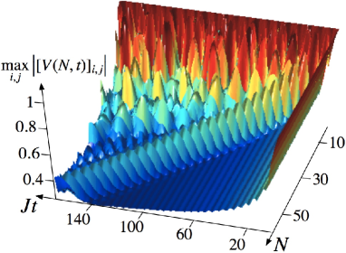
Figure 2: The entries of the matrix governing the dynamics of the system are arbitrarily small—the system is locally arbitrarily close to a Gaussian state—for sufficiently large $N$ and a time interval $[t_{\text{Relax}},t_{\text{Relax}}+t_{\text{Recurrence}}]$ (compare Eq. (24) and Fig. 1). After excitations have traveled through the whole lattice recurrences occur at $t=t_{\text{Recurrence}}$, which is given by the speed of sound. For $N\rightarrow\infty$ no recurrences occur, $t_{\text{Recurrence}}\rightarrow\infty$, and locally the system relaxes to a Gaussian for large times.

Combining both bounds we find that for all $i,j$ (see Fig. 2, where we plot $\max_{i,j}|V_{i,j}|$ versus $N$ and $t$)

$$\left|V_{i,j}\right|<\epsilon\text{ for all }t:\frac{4}{\epsilon^{3}}<Jt<\frac{N}{4\pi^{2}}\frac{\epsilon^{2}}{8\epsilon+6}.$$ (24)

For any $\epsilon>0$, this provides sufficient conditions for satisfying $|V_{i,j}|<\epsilon$ for all $i,j$ and finite $N$ and $t$. This ends step (iii), the intuition of which is summarized in Fig. 1.

We now turn to our original aim, that of showing that the characteristic function $\chi_{i}$ tends to a Gaussian in $\alpha$. The steps in the proof follow the basic structure of the classical proof of the central limit theorem Williamsbook . We start by taking the logarithm of the right hand side of Eq. (14). Expanding the logarithm, we then make use of the observations on $|V_{i,j}|$ obtained above, together with certain properties of Laguerre polynomials.

We can always find appropriate $t$ and $N$ such that $0<L_{m}(|\beta_{i,j}|^{2})\leq 1$ as $|\beta_{i,j}|$ can be made arbitrarily small for given $\alpha$ and all $i,j$, see Eq. (24). Thus we may write

$$\log\prod_{j=1}^{N}L_{m}(|\beta_{i,j}|^{2})=-\sum_{j=1}^{N}\sum_{k=1}^{\infty}\frac{\left(1-L_{m}(|\beta_{i,j}|^{2})\right)^{k}}{k}.$$ (25)

The Laguerre polynomials are defined as

$$L_{m}(x)=\sum_{n=0}^{m}{m\choose m-n}\frac{(-x)^{n}}{n!}=:1-mx+l_{m}(x),$$ (26)

where we defined $l_{m}(x)$ for later use. Hence

$$\log\prod_{j=1}^{N}L_{m}(|\beta_{i,j}|^{2}) = -m\sum_{j=1}^{N}|\beta_{i,j}|^{2}+\sum_{j=1}^{N}l_{m}(|\beta_{i,j}|^{2})$$ (27)

$$- \sum_{j=1}^{N}\sum_{k=2}^{\infty}\frac{\left(1-L_{m}(|\beta_{i,j}|^{2})\right)^{k}}{k}.$$

From the definition of $\beta_{i,j}$ and the unitarity of $V$, the first summation evaluates to $-m|\alpha|^{2}$, which is quadratic as desired, and the remainder of the proof consists of showing that the remaining terms tend to zero for given $\alpha$.

Since $|\beta_{i,j}|=|\alpha V_{i,j}|$, we may use the results above to ensure that for any fixed $\alpha$ the $|\beta_{i,j}|$ are as small as desired, and in particular we shall first suppose that $|\beta_{i,j}|<1$. In this case we have $|l_{m}(|\beta_{i,j}|^{2})|\leq|\beta_{i,j}|^{4}l_{m}(-1)$, and it follows that

$$\begin{split}\left|\sum_{j=1}^{N}l_{m}(|\beta_{i,j}|^{2})\right|&\leq l_{m}(-1)|\alpha|^{4}\sum_{j=1}^{N}\left|V_{i,j}\right|^{4}\\ &\leq l_{m}(-1)|\alpha|^{4}\sup_{i,j}\left|V_{i,j}\right|^{2}\\ &=:l_{m}(-1)|\alpha|^{4}\bar{V}.\end{split}$$ (28)

The large $N$ behavior of this term will evidently be determined by the corresponding behavior of $\bar{V}$, for which we already know that it tends to zero if we first let $N$ and then $t$ go to infinity, see Eq. (24).

Now we study the last term in Eq. (27):

$$\begin{split}&\left|-\sum_{k=2}^{\infty}\frac{(1-L_{m}(|\beta_{i,j}|^{2}))^{k}}{k}\right|\\ &=(1-L_{m}(|\beta_{i,j}|^{2})\sum_{k=1}^{\infty}\frac{(1-L_{m}(|\beta_{i,j}|^{2}))^{k}}{k+1}\\ &\leq-\left(1-L_{m}(|\beta_{i,j}|^{2})\right)\log L_{m}(|\beta_{i,j}|^{2}).\end{split}$$ (29)

By again expanding the Laguerre polynomial as above we have

$$-\log L_{m}(|\beta_{i,j}|^{2}) \leq -\log\left(1-m|\beta_{i,j}|^{2}-|l_{m}(|\beta_{i,j}|^{2})|\right)$$ (30)

$$\leq -\log\left(1-|\alpha|^{2}\bar{V}(m+l_{m}(-1))\right)$$

$$=: \Lambda,$$

which is a sensible bound if we require that $|\alpha|^{2}\bar{V}(m+l_{m}(-1))<1$, which can again be ensured with appropriate $N$ and $t$. Furthermore, $\bar{V}\rightarrow 0$, i.e., also $\Lambda\rightarrow 0$. We thus finally obtain the upper bound

$$\Lambda\sum_{j=1}^{N}\left(1-L_{m}(|\beta_{i,j}|^{2})\right) =\Lambda\sum_{j=1}^{N}\left(m|\beta_{i,j}|^{2}-l_{m}(|\beta_{i,j}|^{2})\right)$$ (31)

$$\leq\Lambda\left(m|\alpha|^{2}+|\alpha|^{4}\bar{V}l_{m}(-1)\right)$$

for the absolute value of the last term in Eq. (27).

Equipped with these bounds, we arrive at the desired statement: We find for any $\alpha\in\mathbb{C}$,

$$\chi_{i}(\alpha;N,t)=\mathrm{e}^{-\left(m+1/2\right)|\alpha|^{2}}+f(\alpha;N,t),$$ (32)

where $|f(\alpha;N,t)|$ can be made arbitrarily small for all $t\in[t_{\text{Relax}},t_{\text{Recurrence}}+t_{\text{Relax}}]$ and a suitable choice of the lattice size $N$, see Eq. (24). Since pointwise closeness for the characteristic functions of two quantum states translates to closeness in trace norm for the states themselves Cushen ; Trace , we have completed the argument for a single site.

We therefore find that the state of a single site, in the limit of large $t$, maximises the entropy for the given initial second moments: Gaussian states have this extremal property of having maximal entropy. Another way of saying this is that, subject to this constraint, it is maximally entangled with the rest of the chain. Since we can bound the time scale on which relaxation occurs – the single site relaxes to a Gaussian state at the rate $(2Jt)^{-1/3}$ – our argument is robust under small perturbations.

This result also gives a clear handle on the situation for finite system sizes: For any finite system size $N$, there will of course eventually be recurrences. The time scale for such recurrences to occur in the $(N,t)$ plane is governed by the speed of sound and the system size $N$: when $t<cN$, where $c$ is the speed of sound, there will be no recurrences, and our argument will apply, giving rise to the time $t_{\text{Recurrence}}$, see Eq. (24). Thus we also arrive at a precise way to describe relaxation for infinite system size: locally the system “looks exactly relaxed” for large times, apparently giving the impression of an “irreversible dynamics”. The same result also holds for correlation functions. This local relaxation is perfectly consistent with the unitary dynamics of the full system; the whole system never truly relaxes to an equilibrium state as it must always preserve the full memory of the initial condition.

The Gaussian character of the state can also be viewed as resulting from a different type of central limit theorem (cf. Ref. Wolf ). The intuition is that time evolution can be thought of as a sequence of of beam splitters acting in parallel, i.e. a quantum quincunx or Galton’s board (this follows from the fact that the dynamics are well-approximated by a quantum cellular automaton). After the bosons bounce through the quincunx we should arrive at a Gaussian characteristic function in phase space describing the state of any single site.

IV Relaxation of blocks

The equilibration for multiple sites, which includes blocks of lattice sites, may be shown using identical techniques, and here we briefly describe the necessary, but minor, modifications. The characteristic function as a function of $\boldsymbol{\alpha}=(\alpha_{1},\ldots,\alpha_{s})^{T}\in\mathbbm{C}^{s}$ for a set of sites $S=[1,\dots,s]$ with reduced state $\hat{\varrho}_{S}$ is defined as

$$\chi_{S}(\boldsymbol{\alpha})=\operatorname{tr}\left[\hat{\varrho}_{S}(N,t)\mathrm{e}^{\sum_{i=1}^{s}(\alpha_{i}\hat{b}_{i}^{\dagger}-\alpha_{i}^{*}\hat{b}_{i}})\right].$$ (33)

After the quench the time-evolving bosonic operators are given by Eq. (10), and the characteristic function becomes

$$\chi_{S}(\boldsymbol{\alpha};N,t)=\mathrm{e}^{-\boldsymbol{\alpha}^{\dagger}\boldsymbol{\alpha}/2}\prod_{j=1}^{N}L_{m}(|\beta_{S,j}(N,t)|^{2}),$$ (34)

where the $\beta_{S,j}$ are now given by $\sum_{i=1}^{s}\alpha_{i}V_{i,j}(N,t)$. Note that otherwise Eq. (14) is unchanged, and the argument can be followed as before to show pointwise convergence in $\boldsymbol{\alpha}$. Using arguments essentially identical to the ones in the proof for a single site, we find in the same sense a convergence

$$\hat{\varrho}_{S}(N,t)\rightarrow\hat{\varrho}_{G}^{\otimes s}$$ (35)

for large times $t$ and large system sizes $N$. That is, the block tends to a product of maximal entropy states.

V Comparison with thermal states

Let us contrast the state arising from our dynamical relaxation with the thermal Gibbs state $\mathrm{e}^{-(\hat{H}_{\text{SF}}-\mu\hat{N})/T}/\operatorname{tr}[\mathrm{e}^{-(\hat{H}_{\text{SF}}-\mu\hat{N})/T}]$ (setting $k_{B}=1$) of the new Hamiltonian $\hat{H}_{\text{SF}}$: for a thermal state at temperature $T>0$, we find the correlations Marcus

$$\langle\hat{b}_{i}^{\dagger}\hat{b}_{j}\rangle=\left[(\mathrm{e}^{(\mathcal{J}-\mu\mathbbm{1})/T}-\mathbbm{1})^{-1}\right]_{i,j}.$$ (36)

The thermal state of $\hat{H}_{\text{SF}}$ is always correlated for all temperatures $T>0$ and all chemical potentials $\mu$ fixing the particle number. In other words, although the system does mix and we do arrive at a state with local maximal entropy, it does not relax to the thermal state of the new Hamiltonian: the conserved second moments prevent this from happening. The relaxation should be thought of as resulting from a mixing process rather than of a physical thermalisation process. Of course the second moments are locally preserved by the dynamics, so under this constraint the entropy is indeed maximised.

VI More general initial states

In fact, an argument along the lines of the above proof can be carried out whenever the the initial state has sufficiently rapidly decaying correlations, reminiscent of the situation in the classical case Spohn . Details of this argument will be presented elsewhere Preparation . For the purposes of this article, we will now consider more general initial states of the form $\otimes_{i=1}^{N}|m_{i}\rangle$, allowing for different particle numbers at different sites – allowing, e.g., for configurations occurring in harmonic traps and periodic distributions with periodicity different from one (realized, e.g., by superimposing a second lattice with different wavelength), reminding of charge density wave or checkerboard phases. For these inhomogeneous initial states the second moments are no longer preserved, but for certain initial states we can nevertheless prove a convergence of second moments. While convergence of second moments is necessary for a local relaxation, it is certainly not sufficient. However, as before, we show that local states relax to a Gaussian state – we show that the characteristic function of the state tends to a Gaussian in $\boldsymbol{\alpha}$ as higher cumulants can be shown to vanish just like in the homogeneous case. For initial states $|\psi(N,0)\rangle=\otimes_{i=1}^{N}|m_{i}\rangle$, the expression for the characteristic function is

$$\chi_{S}(\boldsymbol{\alpha};N,t)=\mathrm{e}^{-\boldsymbol{\alpha}^{\dagger}\boldsymbol{\alpha}/2}\prod_{j=1}^{N}L_{m_{j}}(|\beta_{S,j}(N,t)|^{2}),$$ (37)

with $|\beta_{S,j}|$ as above. Eqs (28-LABEL:eq:sum_fm_bound) and the surrounding discussion must then be modified to incorporate the different $m_{j}$, for example in the quantities $l_{m}(-1)$. All such quantities can be appropriately modified by taking their supremum over all the different $m_{j}$. We then find pointwise convergence of the characteristic function to

$$\lim_{t\rightarrow\infty}\lim_{N\rightarrow\infty}\chi_{S}(\boldsymbol{\alpha};N,t)=\mathrm{e}^{-\boldsymbol{\alpha}^{\dagger}\boldsymbol{\alpha}/2}$$

$$\hskip 28.45274pt\times\exp\Bigl{(}-\lim_{t\rightarrow\infty}\lim_{N\rightarrow\infty}\sum_{j=1}^{N}m_{j}|\beta_{S,j}|^{2}\Bigr{)},$$ (38)

showing that there can be initial configurations for which the state never relaxes. For initial states with $m_{j}=m$ for almost all $j$, we always find relaxation to a steady state as we also do for $P$-periodic initial configurations: Consider an initial state with $m_{i}=m_{i-P}$, completely determined by $m_{1},\dots,m_{P}$. Then, for a block $S$ of $s$ sites,

$$\sum_{j=1}^{N}m_{j}|\beta_{S,j}|^{2}=\sum_{k,l=1}^{s}\alpha_{k}\alpha_{l}^{*}\sum_{p=1}^{P}m_{p}\sum_{j=0}^{N/P-1}V_{k,Pj+p}^{*}V_{l,Pj+p}.$$ (39)

Now,

$$\sum_{j=0}^{N/P-1}V_{k,Pj+p}^{*}V_{l,Pj+p} = \frac{1}{N^{2}}\sum_{r,s=1}^{N}\mathrm{e}^{\mathrm{i}t(\lambda_{r}-\lambda_{s})}\mathrm{e}^{2\pi\mathrm{i}(rl-sk)/N}$$ (40)

$$\times \sum_{j=0}^{N/P-1}\mathrm{e}^{2\pi\mathrm{i}Pj(r-s)/N},$$

and the last terms evaluate to a comb of Kronecker deltas,

$$\sum_{j=0}^{N/P-1}\mathrm{e}^{2\pi\mathrm{i}Pj(r-s)/N}=\frac{N}{P}\sum_{z=-P+1}^{P-1}\delta_{r-s,zN/P},$$ (41)

which yields

$$\sum_{j=0}^{N/P-1}V_{k,Pj+p}^{*}V_{l,Pj+p}=\frac{\delta_{k,l}}{P}+\frac{1}{P}\sum_{\begin{subarray}{c}z=-P+1\\ z\neq 0\end{subarray}}^{P-1}\mathrm{e}^{\pi\mathrm{i}(\frac{z}{P}(l+k)+\frac{l-k}{4})}$$

$$\hskip 28.45274pt\times\frac{1}{N}\sum_{r=1}^{N}\mathrm{e}^{-2\mathrm{i}t\sin(\pi z/P)\lambda_{r}}\mathrm{e}^{2\pi\mathrm{i}r(l-k)/N}.$$ (42)

Identifying the last line with $[V(N,-2t\sin(\pi z/P))]_{l,k}$, which tends to zero as $t$ and $N$ become large (see the proof for the relaxation of a single site), we find also in this scenario that the characteristic function tends to a Gaussian:

$$\lim_{t\rightarrow\infty}\lim_{N\rightarrow\infty}\chi_{S}(\alpha;N,t)=\mathrm{e}^{-(1/2+\bar{m})\boldsymbol{\alpha}^{\dagger}\boldsymbol{\alpha}},\;\;\hat{\varrho}_{S}\rightarrow\hat{\varrho}_{G}^{\otimes s},$$ (43)

where $\bar{m}=\sum_{p=1}^{P}m_{p}/P$. While initially different sites are uncorrelated, correlations build up over time and finally go to zero for large times (see Fig. 3) and the local state relaxes to a direct product of the same Gaussian at each site.

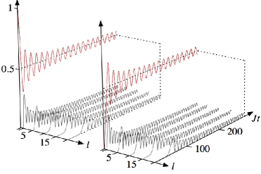
Figure 3: Second moments $\langle\hat{b}_{1}^{\dagger}\hat{b}_{1+l}\rangle$ (left) and $\langle\hat{b}_{2}^{\dagger}\hat{b}_{2+l}\rangle$ (right), $l=0,1,5,10,15,20$, for an initial periodic configuration $|0,1,0,1,\cdots,0,1\rangle$ on a lattice of size $N=300$. For larger times recurrences occur (not shown), while for $N\rightarrow\infty$, one has $\lim_{t\rightarrow\infty}\langle\hat{b}_{i}^{\dagger}\hat{b}_{j}\rangle=\delta_{i,j}/2$.

VII Integrable spin models and fermions

To further illustrate the generality of our approach, we sketch the situation in other integrable models. We consider a $XY$ spin chain,

$$\hat{H}=-\frac{1}{2}\sum_{\langle i,j\rangle}\left(\frac{1+\gamma}{4}\hat{\sigma}_{i}^{x}\hat{\sigma}_{j}^{x}+\frac{1-\gamma}{4}\hat{\sigma}_{i}^{y}\hat{\sigma}_{j}^{y}\right)-\frac{\lambda}{2}\sum_{i=1}^{N}\hat{\sigma}_{i}^{z},$$ (44)

again in the setting of a quenched interaction. By virtue of the familiar Jordan-Wigner transformation, the Hamiltonian is equivalent to a system of spinless fermions:

$$\hat{H}=\frac{1}{2}\sum_{i,j}\left(\hat{f}_{i}^{\dagger}A_{i,j}\hat{f}_{j}-\hat{f}_{i}A_{i,j}\hat{f}_{j}^{\dagger}+\hat{f}_{i}B_{i,j}\hat{f}_{j}-\hat{f}_{i}^{\dagger}B_{i,j}\hat{f}_{j}^{\dagger}\right),$$ (45)

where $A_{i,i}=\lambda$, $A_{i,j}=-1/2$ for $\text{dist}(i,j)=1$, $B_{i,j}=-B_{j,i}=\gamma/2$ for $\text{dist}(i,j)=1$ and zero otherwise.

We start with the system initially in one of the states $|m\rangle^{\otimes N}$, $m=0,1$, corresponding to the magnetized spin states $|\!\!\!\downarrow\rangle^{\otimes N}$, $|\!\!\!\uparrow\rangle^{\otimes N}$, and study time evolution under the above Hamiltonian. As the initial states are fermionic Gaussian states, the system stays Gaussian for all times $t$. Hence, we only need to consider seconds moments, which are most conveniently written in terms of Majorana operators, $\hat{m}_{i}=(\hat{f}_{i}+\hat{f}_{i}^{\dagger})/\sqrt{2}$, $\hat{m}_{N+i}=\mathrm{i}(\hat{f}_{i}^{\dagger}-\hat{f}_{i})/\sqrt{2}$. Then one may collect second moments in a correlation matrix $\gamma(N,t)$ with entries $[\gamma(N,t)]_{i,j}=\text{tr}[\hat{\varrho}(N,t)\hat{m}_{i}\hat{m}_{j}]$. Time evolution of the initial state $|m\rangle^{\otimes N}$ under the above Hamiltonian then amounts to

$$\gamma(N,t)=\mathrm{e}^{tH}\gamma(N,0)\mathrm{e}^{-tH},\,H=\left[\begin{array}[]{cc}0&V\\ -V^{T}&0\end{array}\right],$$ (46)

where $V=A+B$ with eigenvalues

$$\lambda_{k}(V)=\lambda-\cos(2\pi k/N)-\mathrm{i}\gamma\sin(2\pi k/N).$$ (47)

A tedious but elementary calculation delivers the resulting second moments

$$\gamma(N,t)=\frac{1}{2}\left[\mathbbm{1}+\mathrm{i}(-1)^{m}\left(\begin{array}[]{cc}M_{1}(N,t)&M_{2}(N,t)\\ -M_{2}^{T}(N,t)&M_{1}^{T}\end{array}\right)\right],$$ (48)

where

$$M_{1}(N,t) = \sin(2|V|t)\frac{B}{|V|},$$ (49)

$$M_{2}(N,t) = \mathbbm{1}+\sin^{2}(|V|t)\left(\frac{V^{2}}{|V|^{2}}-\mathbbm{1}\right),$$ (50)

from which we immediately see that for the isotropic $XY$ model ($\gamma=0$) second moments are a constant of motion, $\gamma(N,t)=\gamma(N,0)$. We assume $\gamma\neq 0$ from now on. Obviously, as in the bosonic case, the total state stays pure for all times and its entropy is thus always zero, however, depending on the system parameters (it will turn out that it depends on whether the system being quenched to is critical or not – in contrast to the bosonic case, where relaxation occurs independent of the system being critical or not), we find exact relaxation of second moments. To this end, consider the second moments of the state of a single site, $\hat{\varrho}_{i}(N,t)=\text{tr}_{L\setminus\{i\}}[\hat{\varrho}(N,t)]$. It is completely determined by the reduction of the correlation matrix to site $i$, i.e., we need to consider $[M_{1}(N,t)]_{i,i}$ and $[M_{2}(N,t)]_{i,i}$. As the matrices $A$ and $B$ commute and $M_{1}(N,t)$ is the product of a symmetric and an antisymmetric matrix, we immediately find $[M_{1}(N,t)]_{i,i}=0=[M_{1}(N,0)]_{i,i}$. For the sake of clarity, we now focus on the Ising model, $\gamma=1$. It should be clear how the following arguments may be extended to explore the full parameter space. We find

$$\begin{split}\left[M_{2}(N,t)-\mathbbm{1}\right]_{i,i}&=\frac{1}{N}\sum_{k=1}^{N}\sin^{2}(|\lambda_{k}|t)\left(\frac{\lambda_{k}^{2}}{|\lambda_{k}|^{2}}-1\right)\\ &=\frac{1}{N}\sum_{k=1}^{N}\sin^{2}(|\lambda_{k}|t)\frac{\mathrm{e}^{4\pi\mathrm{i}k/N}-1}{1-\lambda\mathrm{e}^{2\pi\mathrm{i}k/N}}.\end{split}$$ (51)

Let us illustrate this for one particular non-critical case, namely $\lambda=0$, for which one has $\lambda_{k}(V)=-\mathrm{e}^{2\pi\mathrm{i}k/N}$ and hence

$$\left[M_{2}(N,t)\right]_{i,i}=1-\sin^{2}(t),$$ (52)

which never relaxes.

It turns out that for the non-critical case, $|\lambda|\neq 1$, the system never locally relaxes. This is, of course, no surprise: in the case where $\lambda=0$ the Hamiltonian we quench to contains only commuting terms. Physically, one of three different processes can take place. In the first case, $\lambda<1$, the system is quenched to a state in the same phase. In this case we do not expect local relaxation as the density of quasiparticles of, eg., $|\!\!\downarrow\rangle^{\otimes m}$ with respect to the new Hamiltonian is too low: there are not enough quasiparticles to lead to an averaging effect. In the critical case $\lambda=1$, the quasiparticles are delocalised and we expect that the density of quasiparticles in $|\!\!\downarrow\rangle^{\otimes m}$ is high enough to lead to a local relaxation. Finally, in the case $\lambda>1$, the quasiparticles of the new system are strongly localised, and appear as pairs in the state $|\!\!\downarrow\rangle^{\otimes m}$ which then oscillate locally.

Let us now turn to the critical case $\lambda=1$, where we expect relaxation. We find

$$\left[M_{2}(N,t)-\mathbbm{1}\right]_{i,i}=-\frac{1}{N}\sum_{k=1}^{N}\sin^{2}(2t\sin(\pi k/N)),$$ (53)

$$- \frac{1}{N}\sum_{k=1}^{N}\sin^{2}(2t\sin(\pi k/N))\mathrm{e}^{2\pi\mathrm{i}k/N},$$

where the first term approaches $-1/2$ and the second term goes to zero for large $N$, $t$, i.e., indeed, at each site the system relaxes when evolved in time under this critical Hamiltonian.

VIII Summary and discussion

In this work, we have investigated the relaxation of Bose-Hubbard type systems and related models following a sudden quench. The intuition we developed was that within a causal cone of neighboring lattice sites, the incommensurate influence of the propagating quasiparticles will give rise to a relaxation dynamics. We have considered a setting in which we could prove an exact local relaxation to a maximal entropy state, providing a guideline of what is expected to happen in similar cases. Also, a precise understanding follows for the scaling of this effect in the system size, as well as of relaxation times. Indeed, the system “looks” perfectly relaxed, while at the same time keeping a perfect memory of the initial situation. We hence can clarify the difference between an apparent – which does happen – and an actual global – which does not happen (!) – relaxation. The argument presented here is expected to be valid whenever the initial condition is sufficiently clustering, so if one has an appropriate decay of correlations.

From the perspective of kinematical approaches to quantum statistical problems, one can interpret our results as follows: When randomizing over all possible pure states Winter , the local state will have maximal entropy for large systems. Here, we arrive at the same result, but not by a kinematical argument, but via a dynamical argument, where the mixing is achieved through local physical dynamics in a lattice system. It would be interesting to further try to combine the kinematical and dynamical pictures for more general Hamiltonians.

Settings similar to those discussed here are readily accessible in experiments using ultracold bosonic atoms in optical lattices Experiments , and this is what motivates this work. The general guideline is that local or correlation functions will relax. Most accessible would be a situation where only second moments would have to be monitored, starting, e.g., with a checkerboard type situation of alternating occupation numbers in a Mott state (cp. Section VI and Fig. 3), prepared using two distinct optical lattices in a spatial dimension. The idealized case of a vanishing interaction $U$ gives rise to a guideline for what to expect in realistic settings and also to a general principle: the local relaxation conjecture. It is our hope that the present work fosters further experiments along these lines.

- (1) M. Greiner, O. Mandel, T. W. Hänsch, and I. Bloch, Nature 419, 51 (2002); A.K. Tuchman, C. Orzel, A. Polkovnikov, and M.A. Kasevich, cond-mat/0504762; T. Kinoshita, T. Wenger, and D.S. Weiss, Nature 440, 900 (2006); L.E. Sadler, J.M. Higbie, S.R. Leslie, M. Vengalattore, and D.M. Stamper-Kurn, Nature 443, 312 (2006).
- (2) M.J. Hartmann, G. Mahler, and O. Hess, Phys. Rev. E 70, 066148 (2004).
- (3) D.N. Page, Phys. Rev. Lett. 71, 1291 (1993); S. Popescu, A.J. Short, and A. Winter, Nature Physics 2, 754 (2006); A. Serafini, O.C.O. Dahlsten, and M.B. Plenio, J. Phys. A 40, 9551 (2007); D. Gross, K. Audenaert, and J. Eisert, J. Math. Phys. 48 (2007).
- (4) D.C. Brody, D.W. Hook, and L.P. Hughston, J. Phys. A 40, F503 (2007).
- (5) K. Sengupta, S. Powell, and S. Sachdev, Phys. Rev. A 69, 053616 (2004); J. Berges, S. Borsanyi, and C. Wetterich, Phys. Rev. Lett. 93, 142002 (2004); S.O. Skrøvseth, Europhys. Lett. 76, 1179 (2006); M.A. Cazalilla, Phys. Rev. Lett. 97, 156403 (2006); C. Kollath, A. Läuchli, and E. Altman, Phys. Rev. B 74, 174508 (2006).
- (6) W.H. Zurek, U. Dorner, and P. Zoller, Phys. Rev. Lett. 95, 105701 (2005).
- (7) E. Perfetto, Phys. Rev. B 74, 205123 (2006).
- (8) K. Rodriguez, S.R. Manmana, M. Rigol, R.M. Noack and A. Muramatsu, New J. Phys. 8, 169 (2006); M. Rigol, A. Muramatsu, and M. Olshanii, Phys. Rev. A, 74, 053616 (2006); M. Rigol, V. Dunjko, V. Yurovsky, and M. Olshanii, cond-mat/0604476 (2006).
- (9) S.R. Manmana, S. Wessel, R.M. Noack, and A. Muramatsu, Phys. Rev. Lett. 98, 210405 (2007).
- (10) J. Eisert and T.J. Osborne, Phys. Rev. Lett. 97, 150404 (2006); S. Bravyi, M.B. Hastings, and F. Verstraete, ibid. 97, 050401 (2006); G. De Chiara, S. Montangero, P. Calabrese, and R. Fazio, J. Stat. Mech. 0603, P001 (2006).
- (11) I. Peschel and V. Eisler, private communication (2006).
- (12) J. Eisert, M.B. Plenio, S. Bose, and J. Hartley, Phys. Rev. Lett. 93, 190402 (2004); M.B. Plenio, J. Hartley, and J. Eisert, New J. Phys. 6, 36 (2004); M.J. Hartmann, M.E. Reuter, and M.B. Plenio, ibid. 8, 94 (2006).
- (13) P. Calabrese and J. Cardy, Phys. Rev. Lett. 96, 136801 (2006), cond-mat/0601225
- (14) O.E. Lanford, III, and D.W. Robinson, Commun. Math. Phys. 24, 193 (1972).
- (15) T.V. Dudnikova, A.I. Komech, and H. Spohn, J. Math. Phys. 44, 2596 (2003).
- (16) D. Jaksch, C. Bruder, J.I. Cirac, C.W. Gardiner, and P. Zoller, Phys. Rev. Lett. 81, 3108 (1998).
- (17) D. Williams, Probability with martingales (Cambridge University Press, Cambridge, 1991).
- (18) S.M. Barnett and P.M. Radmore, Methods in theoretical quantum optics (Oxford Science Publications, Oxford, 1997).
- (19) L.J. Landau, J. Lond. Math. Soc. 61, 197 (2000).
- (20) G.N. Watson, A treatise on the theory of Bessel functions, (Cambridge University Press, Cambridge, 1944).
- (21) G. Kuperberg, math-ph/0202035.
- (22) M. Cramer and J. Eisert, New J. Phys. 8, 71 (2006).
- (23) M.M. Wolf, G. Giedke, and J.I. Cirac, Phys. Rev. Lett. 96, 080502 (2006).
- (24) E.B. Davies, Commun. Math. Phys. 15, 277 (1969); 27, 309 (1972).
- (25) C. D. Cushen and R. L. Hudson, J. Appl. Prob. 8, 454 (1971).
- (26) In preparation.