Lyapunov instability of rigid diatomic molecules in three dimensions - a simpler method

Abstract

We present a new method to calculate Lyapunov exponents of rigid diatomic molecules in three dimensions ($12N$ dimensional phase space). The spectra of Lyapunov exponents are obtained for 32 rigid diatomic molecules interacting through the Weeks-Chandler-Anderson(WCA) potential for various bond length and densities, and compared with those in Y.-H. Shin et al.shin01 . Our algorithm is easy to implement and total CPU time is relatively inexpensive.

I Introduction

One of the ways to quantify the dynamical instability of a many-body system is to examine its Lyapunov exponents. Lyapunov exponents are a measure of the average rate at which nearby trajectories converge or diverge in the phase spacegaspard98 ; hoover99 ; dorfman99 . A positive Lyapunov exponent indicates a divergence between nearby trajectories, i.e., a high sensitivity to initial conditions. There are various methods to compute Lyapunov exponents in the literaturezeng91 ; christiansen97 ; rangarajan98 ; ramasubramanian99 ; posch06 .

In this paper we propose a new method to calculate Lyapunov exponents of the rigid diatomic molecules in three dimensions, which does not require periodic rescaling of the bond length. Rigid diatomic molecules are often described by hard dumbbells and there have been several works on the Lyapunov instability for the diatomic molecular modelsborzsak96 ; dellago97 ; milanovic98 ; milanovic98b ; kum98 ; shin01 ; milanovic02 .

Our method is based on the algorithms proposed by Omelyan et al.omelyan02 . They proposed the optimized Verlet-like algorithms which are derived on the basis of an extended decomposition scheme at the presence of a free parameter and which are more efficient than the original Verlet versions that corresponds to a particular case when the introduced parameter is equal to zero.

In the present paper, we extend Omelyan’s algorithms to the calculation of Lyapunov exponents, and show that our algorithm works efficiently. We compare present results with those appeared in Ref.shin01 , which uses two coordinates representations to avoid the singularity occurring in the equations of motion by combining with the adaptive Runge-Kutta-Fehlberg method of order four.

II Equations of motion

The position and the orientation of the diatomic molecule are specified by a vector to the center of mass, $\vec{q}$, and a unit vector which points along the molecular axis. We denote this unit vector by $\vec{S}$. Then, the equations of motion are chen01

$$\dot{\vec{q}} = {\vec{p}\over M},$$

$$\dot{\vec{p}} = -{\partial V\over\partial\vec{q}},$$

$$\dot{\vec{S}} = {1\over I}\vec{L}\times\vec{S}=\vec{\omega}\times\vec{S},$$

$$\dot{\vec{L}} = -\vec{S}\times{\partial V\over\partial\vec{S}},$$ (1)

where $\vec{p}$ represents the momentum, $M$ the total mass of the molecule, $I$ the moment of inertia, and $\vec{L}$ the angular momentum. As in the Verlet algorithm, we split the Hamiltonian for rigid diatomic molecular motion into kinetic and potential parts: $H=T+V$, where $T={1\over 2M}\vec{p}\cdot\vec{p}+{1\over 2I}\vec{L}\cdot\vec{L}$ and $V=V(\vec{q},\vec{S})$. The Weeks-Chandler-Anderson(WCA) potential with a cutoff length $r_{c}$ = 2^1/6 is used as the intermolecular potential function. It should be noted that the previous work on the system composed of hard dumbellsmilanovic98 employs more complicated algorithm because of the discontinuity imposed on the interaction potential. In the present work, all the numerical results are based on the simulations performed on the system composed of 32 diatomic molecules.

The exact solutions with initial condition $\vec{x}_{0}=(\vec{q}_{0},\vec{p}_{0},\vec{S}_{0},\vec{L}_{0})$ are given as follows.

1. Motion induced by $V$ :

$${\rm exp_{V}(t)}\vec{x}_{0}=\left(\vec{q}_{0},~{}\vec{p}_{0}-t{\partial V\over\partial\vec{q}}|_{\vec{x}_{0}},~{}\vec{S}_{0},~{}\vec{L}_{0}-t\vec{S}_{0}\times{\partial V\over\partial\vec{S}}|_{\vec{x}_{0}}\right).$$ (2)

2. Motion induced by $T$ :

$${\rm exp_{T}(t)}\vec{x}_{0}=\left(\vec{q}_{0}+{t\over M}\vec{p}_{0},~{}\vec{p}_{0},~{}\vec{S^{\prime}},~{}\vec{L}_{0}\right),$$ (3)

where we use the algorithm in Ref.omelyan01 to update $\vec{S}$

$$\vec{S^{\prime}}={(\vec{S}_{0}+(\vec{\omega}\times\vec{S}_{0})\Delta t+{\Delta t^{2}\over 2}[\vec{\omega}(\vec{\omega}\cdot\vec{S}_{0})-{1\over 2}(\vec{\omega}\cdot\vec{\omega})\vec{S}_{0}])\over[1+(\omega\Delta t/2)^{2}]}.$$ (4)

One of great advantages of this algorithm is that we don’t need to adjust the bond length during the simulations. This is also true in Ref.shin01 , where the bond length is naturally fixed without using any additional constraint. However, the equations of motion in our model are much simpler than those used in Ref. shin01 , and they are easy to implement.

A split Hamiltonian scheme for the integration, thus, is given as

$$\left(\vec{q}^{i+1},\vec{p}^{i+1},\vec{S}^{i+1},\vec{L}^{i+1}\right) = {\rm exp_{V}}({1\over 2}\Delta t)~{}{\rm exp_{T}}(\Delta t)~{}{\rm exp_{V}}({1\over 2}\Delta t)\times\left(\vec{q}^{i},\vec{p}^{i},\vec{S}^{i},\vec{L}^{i}\right).$$ (5)

In the actual simulations, however, we use the optimized Verlet-like algorithms proposed recently by Omelyan et al.omelyan02 to get the Lyapunov exponents. In their paper it is shown that the optimized position-Verlet-like(OPV) algorithm is a little more efficient than the optimized velocity-Verlet-like(OVV) algorithm. Thus, we use the OPV algorithm in this paper. The algorithm reads

$$\vec{v}_{I} = \vec{v}(t)+{1\over m}\vec{f}(\vec{r}(t))\xi\Delta t,$$

$$\vec{r}_{I} = \vec{r}(t)+\vec{v}_{I}\Delta t/2,$$

$$\vec{v}_{II} = \vec{v}_{I}(t)+{1\over m}\vec{f}(\vec{r}_{I})(1-2\xi)\Delta t,$$

$$\vec{r}(t+\Delta t) = \vec{r}_{I}(t)+\vec{v}_{II}\Delta t/2,$$

$$\vec{v}(t+\Delta t) = \vec{v}_{II}+{1\over m}\vec{f}(\vec{r}(t+\Delta t))\xi\Delta t,$$ (6)

where the parameter $\xi\approx$ 0.1931833275037836 and $\vec{r}_{I},\vec{r}_{II},\vec{v}_{I}$, and $\vec{v}_{II}$ denote the center of positions and their velocities of a diatomic molecule. Similarly, we have the propagation of the unit vector $\vec{S}$ and angular momentum $\vec{L}$ from time $t$ to $t+\Delta t$. A time step $\Delta t$ = 0.0005 is used in our simulations.

III Lyapunov exponents

The initial configuration of the molecules and the simulation method in Ref.shin01 are used in our simulations. The velocities are repeatedly scaled to adjust the required temperature from sufficiently high temperature . Once the required temperature is obtained, the system is equilibrated for 500 time units (10⁶ iterations), and data is collected for 500 time units(10⁶ iterations) to evaluate the Lyapunov exponents. Below all quantities are given in reduced units.

In order to get the exponents we use the classical method of Benettin at al.benettin76 refined by Hoover and Poschhoover85 ; hoover87 ; posch88 ; posch89 that requires continuous orthonormalization. The corresponding equations for the variation are given as follows.

$$\delta\dot{\vec{q}} = {\delta\vec{p}\over M},$$

$$\delta\dot{\vec{p}} = -\delta{\partial V\over\partial\vec{q}},$$

$$\delta\dot{\vec{S}} = {1\over I}\delta(\vec{L}\times\vec{S})=\delta(\vec{\omega}\times\vec{S}),$$

$$\delta\dot{\vec{L}} = -\delta(\vec{S}\times{\partial V\over\partial\vec{S}}).$$ (7)

It should be noted that we consider only the first order, $\cal{O}$($\Delta t$), for updating $\delta\vec{S}$. In our model we have $12N$ dimensional phase space. In order to compare our results with those from $10N$ dimensional phase space in Ref.shin01 , we subtract the additional two degrees of freedoms in each diatomic molecule. We have two constraints in equations of motion :

$$\vec{S}\cdot\delta\vec{S} = 0,$$ (8)

$$\vec{S}\cdot\delta\vec{L}+\delta\vec{S}\cdot\vec{L} = 0.$$ (9)

These equations are obtained from two conditions : $\vec{S}\cdot\vec{S}$ = 1 (normalization) and $\vec{S}\cdot\vec{L}$ = 0 (orthogonality). In order to fulfill two constraints $\delta\vec{S}$ and $\delta\vec{L}$ are replaced with,

$$\delta\vec{S}\equiv\delta\vec{S}-(\vec{S}\cdot\delta\vec{S})\vec{S},$$ (10)

$$\delta\vec{L}\equiv\delta\vec{L}-(\vec{S}\cdot\delta\vec{L}+\delta\vec{S}\cdot\vec{L})\vec{S},$$ (11)

respectively. Then, $12N$ dimensional phase space can be reduced to $10N$ dimensional one.

We find the characteristic features of the spectra of the Lyapunov exponents in our model are the same as those in Ref.shin01 . In Fig. 1 we compare the positive branch of exponents from our calculation with that from Ref.shin01 at $T$=1.0, $D$=0.3, $B$=1.0, where $T$ is temperature, $D$ is the density, and $B$ is the bond length, respectively. $\lambda_{l}$ is the discrete spectrum of the Lyapunov exponents, and index $l$ represents 1, …, 160, i.e. the half of total number of all phase space variables .

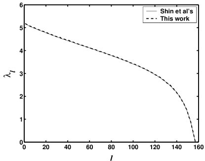
Figure 1: Comparison of the Lyapunov exponents at $T$=1.0, $D$=0.3, $B$=1.0.

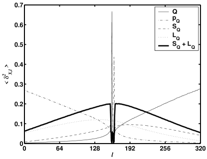
Figure 2: Mean-squared values of the projection at $T$=1.0, $D$=0.3, $B$=1.0.

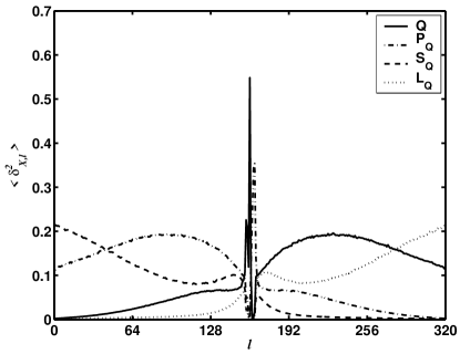
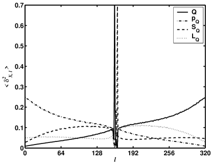
Figure 3: Same as in Fig.2, but at $T$=1.0, $D$=0.3, $B$=0.2 (top), and at $T$=0.1, $D$=0.3, $B$=1.0 (bottom).

Table 1: The largest Lyapunov exponent $\lambda_{1}$ and the smallest positive Lyapunov exponent $\lambda_{156}$, and four vanishing exponents ($\lambda_{157}$, $\lambda_{158}$, $\lambda_{159}$, and $\lambda_{160}$) for various bond length B at a fixed number density D=0.3 (upper) and D=0.5 (lower).

B	0.2		0.4		0.6		0.8		1.0
$\lambda_{1}$	4.320		4.574		4.791		4.989		5.179
$\lambda_{156}$	0.104		0.170		0.274		0.272		0.229
$\lambda_{157}$	0.025		0.046		0.041		0.034		0.030
$\lambda_{158}$	0.018		0.014		0.014		0.017		0.013
$\lambda_{159}$	0.010		0.008		0.012		0.012		0.011
$\lambda_{160}$	0.012		0.009		0.009		0.011		0.007

B	0.2		0.4		0.6		0.8		1.0
$\lambda_{1}$	6.158		6.526		6.557		6.327		5.746
$\lambda_{156}$	0.108		0.113		0.052		0.052		0.032
$\lambda_{157}$	0.068		0.056		0.028		0.015		0.013
$\lambda_{158}$	0.020		0.013		0.015		0.014		0.011
$\lambda_{159}$	0.014		0.011		0.010		0.011		0.012
$\lambda_{160}$	0.010		0.009		0.007		0.010		0.003

Table 1 shows the largest Lyapunov exponents $\lambda_{1}$, the smallest positive Lyapunov exponent $\lambda_{156}$, and four vanishing exponents ($\lambda_{157}$, $\lambda_{158}$, $\lambda_{159}$, and $\lambda_{160}$) for various bond length B at a fixed number density D=0.3, and D=0.5, respectively. Temperature is set to $T$=1.0 for both cases. The same trend for the largest Lyapunov exponent $\lambda_{1}$ was already shown in Ref.shin01 .

On the other hand, the dynamics of the tangent vectors in the subspace are slightly different. We calculate the mean-squared value of the projection of tangent vectors $\delta_{l}$ onto $TX$ subspace which is defined as usual

$$\langle\vec{\delta}^{2}_{X,l}\rangle=\langle\mathcal{P}(X)\vec{\delta}_{l}\cdot\mathcal{P}(X)\vec{\delta}_{l}\rangle.$$ (12)

Fig.2 shows the projection at $T$=1.0, $D$=0.3, $B$=1.0, where $Q$ denotes $x$, $y$, and $z$ components. In our model $\langle\vec{\delta}^{2}_{X,l}\rangle$ for $\vec{S}$ and $\vec{L}$ phase space and their tangent space $\delta\vec{S}$ and $\delta\vec{L}$ are not symmetric with respect to the center. A similar asymmetric behavior was also found in Ref.hoover01 . However, we find the Hamiltonian nature of the system, i.e., an increase of instability accumulated in one subspace is always accompanied with a decrease of instability in its conjugate subspace. In Fig.2 we also show $S_{Q}+L_{Q}$, which is symmetric with respect to the center, for comparison.

It is interesting to note that the overall patterns are symmetric if temperature is low or the bond length is small. In Fig.3 we show the projection at $T$=1.0, $B$=0.2, and at $T$=0.1, $B$=1.0, respectively. The density is set to $D$=0.3 for both cases. It is not clear to us why the projection depends on temperature or the bond length, and symmetry becomes broken as temperature or the bond length is increasing. We speculate that this might come from a relation between $\vec{S}$ and $\vec{L}$. Note that the correct conjugate momentum for rotation ischen01

$$\vec{\Pi}=I\dot{\vec{S}}=\vec{L}\times\vec{S},$$ (13)

not simply $\vec{L}$. More detailed analyses will be needed regarding the asymmetric behavior. It can be shown that the overall patterns are always symmetric if our coordinate system is transformed to that of Ref.shin01 , i.e., ($\vec{q}$, $\vec{p}$, $\theta$, $\phi$, $p_{\theta}$, $p_{\phi}$) (See Fig 4). Clearly, this shows that our coordinate system is consistent with that of Ref.shin01 .

In Table 2 we show comparison of total CPU time for our simulations and Shin et al.’s on the Lyapunov exponents. Our code is relatively inexpensive, although we need to implement two constraints in Eq.(8) and Eq.(9). In Ref.shin01 the coordinate transformation is needed to avoid singularity occurring in the equations of motion, and a sophisticated integrator is used because the coordinate transformation cannot be applied to the calculation of the Lyapunov exponents. These might consume a relatively large CPU time during the simulations.

Table 2: Comparison of total CPU time(in hours) for the simulations on a single node (Intel 3.06GHz CPU).

	This work(A)		Shin et al’s(B)		A/B
T=1.0, D=0.3, B=0.2	8.8h		16.5h		0.53
T=1.0, D=0.3, B=1.0	15.5h		24.6h		0.63
T=1.0, D=0.5, B=0.2	17.1h		28.3h		0.60

In summary, we propose a new approach to calculate Lyapunov exponents of the rigid diatomic molecules in three dimensions, which does not need a rescaling of the bond length, and it is computationally relatively inexpensive.

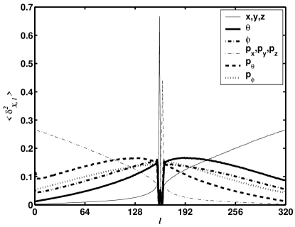
Figure 4: Same as in Fig. 2. After transforming of the coordinate system.

The authors would like to thank Dr. Dong-Chul Ihm for contributing to the early stages of this work. S.C. is grateful to Prof. H.A. Posch for helpful comments in the early stage of this work, and he also thanks Dr. C.-H. Cho and Dr. Y.-H. Shin for useful discussions. This work was supported by the Korea Research Foundation Grant No. KRF-2005-070-C00065.

References

- (1) Y.-H. Shin, D.-C. Ihm, and E.-K. Lee, Phys. Rev. E 64, 041106 (2001).
- (2) P. Gaspard, Chaos, Scattering and Statistical Mechanics, Cambridge University Press, Cambridge, 1998.
- (3) W.G. Hoover, Time Reversibility, Computer Simulation, and Chaos, World Scientific, Singapore, 1999.
- (4) J.R. Dorfman, An Introduction to Chaos in Nonequilibrium Statistical Mechanics, Cambridge University Press, Cambridge, 1999.
- (5) X. Zeng, R. Eykholt, and R.A. Pielke, Phys. Rev. Lett. 66, 3229 (1991).
- (6) F. Christiansen and H.H. Rugh, Nonlinearity 10, 1063 (1997).
- (7) G. Rangarajan, S. Habib, and R.D. Ryne, Phys. Rev. Lett. 80, 3747 (1998).
- (8) K. Ramasubramanian and M.S. Sriram, Phys. Rev E 60, R1126 (1999).
- (9) H.A. Posch and W.G. Hoover, J. Phys. : Conference Series 31, 9 (2006); and references therein.
- (10) I. Borzsák, H.A. Posch, and A. Baranyai, Phys. Rev. E 53, 3694 (1996).
- (11) Ch. Dellago and H.A. Posch, Physica A 237, 95 (1997).
- (12) L. Milanović, H.A. Posch, and W.G. Hoover, Chaos 8, 455 (1998).
- (13) L. Milanović, H.A. Posch, and W.G. Hoover, Molec. Phys. 95, 281 (1998).
- (14) O. Kum, Y.H. Shin, E.K. Lee, Phys. Rev. E 58, 7243 (1998).
- (15) L. Milanović, H.A. Posch, J. Molecular Liquids 96-97, 221 (2002).
- (16) I.P. Omelyan, I.M. Mryglod, and R. Folk, Phys. Rev. E 65, 056706 (2002).
- (17) B. Chen and J.H. Schenker, Applied Numerical Mathematics 38, 21 (2001).
- (18) I.P. Omelyan, I.M. Mryglod, and R. Folk, Phys. Rev. Lett. 86, 898 (2001).
- (19) G. Benettin, L. Galgani, and J.-M. Strelcyn, Phys. Rev. A 14, 2338 (1976).
- (20) W.G. Hoover and H.A. Posch, Phys. Lett. A 113, 82 (1985).
- (21) W.G. Hoover and H.A. Posch, Phys. Lett. A 123, 227 (1987).
- (22) H.A. Posch and W.G. Hoover, Phys. Rev. A 38, 473 (1988).
- (23) H.A. Posch and W.G. Hoover, Phys. Rev. A 39, 2175 (1989).
- (24) W.G. Hoover, H.A. Posch, and C.G. Hoover, J. Chem. Phys. 115, 5744 (2001).