Light-matter interaction in doped microcavities

Abstract

We discuss theoretically the light-matter coupling in a microcavity containing a quantum well with a two-dimensional electron gas. The high density limit where the bound exciton states are absent is considered. The matrix element of interband optical absorbtion demonstrates the Mahan singularity due to strong Coulomb effect between the electrons and a photocreated hole. We extend the non-local dielectric response theory to calculate the quantum well reflection and transmission coefficients, as well as the microcavity transmission spectra. The new eigenmodes of the system are discussed. Their implications for the steady state and time resolved spectroscopy experiments are analyzed.

I Introduction

The phenomena of coherent energy transfer between a microcavity photon and a quantum well exciton have been demonstrated experimentally for the first time in Ref. weisbuch, . Since when the linear and non-linear effects in quantum microcavities are extensively studied both experimentally and theoretically. deveaud_book ; Kavokin and Malpuech (2003)

The strong light-matter interaction manifests itself as the appearance of new eigen-modes, exciton-polaritons, being composite half-light – half-matter particles. The formation of the exciton-polaritons can be understood in the terms of two coupled oscillators describing the confined photon and exciton respectively. If the coupling constant $V_{R}$ exceeds the total damping rate (caused by the photon leakage through the mirrors and the exciton inhomogeneous broadening) two new eignemodes splitted by $2V_{R}$ appear. The microcavity transmission and reflection coefficients as the functions of the excitation energy and the detuning between exciton and photon energies show an anticrossing behavior familiar in the two-level interacting systems, which is the signature of the strong-coupling regime. In time-resolved experiments the coherent beats of emission are observed demonstrating the energy transfer between an exciton and a photon. rabi

The weak doping of the microcavity with electrons is shown to increase the scattering rates of the exciton-polaritons. Kavokin and Malpuech (2003); bloch In the moderate doping conditions where the quantum well absorbtion edge is determined by charged excitons ($X^{+}$ or $X^{-}$ trions), the strong coupling between photon and trion was demonstrated. Qarry et al. (2003) The situation is expected to be drastically different in the highly doped systems. In this case bound exciton states are known to vanish due to both the screening of the Coulomb potential and the state-filling effects, an interband absorbtion is governed by the Mahan singularity. Mahan (1967a); ROULET et al. (1969); Hawrylak (1991) If such a quantum well is embedded into the microcavity, the confined photon interacts with a continuum of states which should lead to the strong differences with the two-oscillator model.

In the present paper we consider the latter regime of light-matter coupling. We calculate the optical susceptibility of a two-dimensional electron gas confined in a quantum well with allowance for the interaction between Fermi-sea of electrons and a photocreated hole. Further, we use the non-local dielectric response theory in order to find the quantum well reflection and transmission coefficients. Then the transfer matrix method is applied to study the steady-state and time-domain responses of a microcavity with a doped quantum well. The results are interpreted in the framework of the simple quantum-mechanical model which describes the coupling between a discrete state (photon) and a continuum of electron-hole excitations.

The paper is organized as follows: an expression for the optical susceptibility of a two-dimensional electron gas with allowance for the Fermi-edge singularity is derived in Sec. II. Section III is devoted to the calculation of a quantum microcavity transmission coefficient. The implications of the Fermi-edge singularity on time-resolved response of the microcavity is discussed in Sec. IV.

II Susceptibility of a doped quantum well

Let us consider a doped quantum well made of a direct band semiconductor with the effective band gap (including quantum well size-quantization energy) $E_{g}$. We assume that the quantum well contains a two-dimensional electron gas with the concentration $N=k_{F}^{2}/2\pi$, where $k_{F}$ is the Fermi wave vector. The gas parameter $r_{s}=\sqrt{2}me^{2}/(\kappa_{0}\hbar^{2}k_{F})$, where $m$ is electron effective mass, $e$ is the elementary charge and $\kappa_{0}$ is the static dielectric constant, characterizes the ratio between the Coulomb interaction energy of electrons and their Fermi energy $E_{F}=\hbar^{2}k_{F}^{2}/2m$. Gas parameter is assumed to be the small parameter of our theory, $r_{s}\ll 1$, i.e. the Coulomb interaction of the Fermi-level electrons is negligible.

The absorbtion of a photon with an energy $\hbar\omega$ in the vicinity of $E_{g}+E_{F}$ creates an extra electron in the conduction band and a hole in the valence band. For simplicity we assume that the hole is infinitely heavy and interacts with electrons by a short range attractive potential $V(\bm{r})=V_{0}\delta(\bm{r})$ ($V_{0}<0$). Latter assumption is violated for the electrons with the wavevectors $k\ll k_{F}$ which form bound states with the hole and screen the long-range Coulomb potential. These bound states, however, have an energy close to $E_{g}$ and do not determine the optical properties of the quantum well for $\hbar\omega\approx E_{g}+E_{F}$. In this spectral range the interband matrix element of the optical absorbtion is strongly modified due to the combined effect of the electron-hole interaction and the step-like change of the density of available states as Mahan (1967a); ROULET et al. (1969); Hawrylak (1991); Pardee and Mahan (1973); Penn et al. (1981)

$$M_{k}=M^{0}_{k}\left(\frac{E_{F}}{\hbar\omega-E_{g}-E_{F}}\right)^{\frac{\delta}{\pi}}.$$ (1)

Here $k=\sqrt{2m(\hbar\omega-E_{g})/\hbar^{2}}$ is the photoexcited electron wavevector, $M^{0}_{k}$ is the bare matrix element (calculated without electron-hole interaction) and the power of singularity $\delta$ is given for the short-range potential by

$$\delta=\delta_{0}-\frac{\delta_{0}^{2}}{\pi},$$ (2)

where $\delta_{0}=-mV_{0}/2\hbar^{2}$ is the scattering phase-shift introduced by a hole in $s$-channel. Pardee and Mahan (1973); anderson67 The first term in Eq. (2) describes an excitonic enhancement of the absorbtion and the second term takes into account the ‘orthogonality catastrophe’: due to the interaction with hole the electron wavefunctions rearrange and become nearly orthogonal to the initial wavefunctions. This expression (1) is valid for $|\hbar\omega-E_{g}-E_{F}|\lesssim E_{F}$, otherwise $M_{k}\approx M^{0}_{k}\approx const$. An extra factor of the order of unity as well as the shift of the absorbtion edge may appear in Eq. (1) in a more elaborate approach. Penn et al. (1981) We disregard it for the purposes of the present paper.

The light matter interaction in the planar systems can be most conveniently described by the non-local dielectric response theory where the quantum well polarization $\bm{P}$, caused by the electromagnetic field $\bm{E}$ incident along the quantum well growth axis $z$, can be represented in the integral form Andreani et al. (1991); Kavokin and Malpuech (2003); Ivchenko (2005)

$$\bm{P}(z)=\int\pi(\omega,z,z^{\prime})\bm{E}(z^{\prime})\mathrm{d}z^{\prime},$$ (3)

where $\pi(\omega,z,z^{\prime})$ is so-called non-local susceptibility. It can be written as a sum over all allowed transitions, i.e.

$$\pi(\omega,z,z^{\prime})=\frac{1}{4}\hbar\kappa_{b}\omega_{LT}a_{B}^{3}\Phi(z)\Phi(z^{\prime})G(\omega),$$ (4)

$$G(\omega)=\frac{1}{\mathcal{S}}\sum_{\bm{k}}\left|\frac{M_{k}}{M_{k}^{0}}\right|^{2}\frac{1-n_{F}(k)}{E_{g}+\frac{\hbar k^{2}}{2m}-\hbar\omega-\mathrm{i}0},$$

where $\mathcal{S}$ is the normalization area, $\kappa_{b}$ is the background high-frequency dielectric constant, $a_{B}$ and $\omega_{LT}=4\hbar e^{2}p_{cv}^{2}/(E_{g}^{2}m_{0}^{2}\kappa_{b}a_{B}^{3})$ are the Bohr radius and longitudinal-transverse splitting of the bulk exciton, $p_{cv}$ is the interband dipole matrix element, $\Phi(z)=\varphi_{e}(z)\varphi_{h}(z)$ is the electron-hole pair envelope along the growth axis, and $n_{F}(k)=1$ for $k\leqslant k_{F}$ and $0$ otherwise is the Fermi distribution function. In Eq. (4) we assumed that the quantum well is thin enough that the Coulomb effect on the motion of electron and hole along $z$ axis can be neglected, we disregarded the inhomogeneous broadening of the electron states, and set temperature to be zero.

Substituting Eq. (1) into Eq. (4) one obtains a closed form expression for the susceptibility for $|\hbar\omega-E_{g}-E_{F}|\lesssim E_{F}$ and $\delta>0$:

$$G(\omega)=\frac{m}{2\hbar^{2}\sin{2\delta}}\left\{\begin{array}[]{cc}\left(-\mathcal{E}\right)^{-\frac{2\delta}{\pi}},&\mathcal{E}<0,\\ e^{2\mathrm{i}\delta}\mathcal{E}^{-\frac{2\delta}{\pi}},&\mathcal{E}>0.\\ \end{array}\right.$$ (5)

Here reduced energy $\mathcal{E}=(\hbar\omega-E_{g}-E_{F})/E_{F}$. One can see that below the threshold, $\mathcal{E}<0$, the susceptibility is real, while above the threshold, $\mathcal{E}>0$, the susceptibility contains both real and imaginary parts. Note that formally the integral describing the real part of $\pi(\omega,z,z^{\prime})$ in (4) is logarithmically divergent as $M_{k}/M^{0}_{k}\to 1$ for $k\to\infty$. To obtain a finite result either non-resonant terms in the susceptibility or corrections to the effective mass method are needed. In the doped system, however, for $\hbar^{2}k^{2}/2m\sim E_{F}$ the broadening of the single particle levels due to electron-electron scattering makes large $k$ contribution negligible and one may use Eq. (1) for the interband matrix element in a whole relevant spectral range.

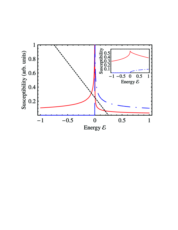
Figure 1: (Color online). Susceptibility of the doped quantum well $G$ [Eq. (5)], plotted as a function of $\mathcal{E}=(\hbar\omega-E_{g}-E_{F})/E_{F}$. Real part is shown by red solid line, blue dash-dot line represents the imaginary part of $G$. Black dotted line shows $\hbar\omega_{c}/E_{F}-\mathcal{E}$ ($\hbar\omega_{c}/E_{F}=0.25$) and the intersection points are the solutions of Eq. (14). The parameters used are: $\delta=0.63$, dimensionless light-matter coupling constant $\mathcal{C}=0.1$. An inset shows susceptibility calculated for negative value of $\delta=-0.63$.

If the enhancement power $\delta=0$ then the power-law singularity in susceptibility is replaced by the logarithmic one, $G(\omega)\propto\ln{(-\tilde{\mathcal{E}}/\mathcal{E})}$, where $\tilde{\mathcal{E}}$ is the cut-off energy. ivchenkopikus In the case of negative power $\delta<0$ in Eq. (1) the singularity is absent

$$G(\omega)=\frac{m}{2\hbar^{2}}\left\{\begin{array}[]{cc}\Gamma{\left(1-\frac{2\delta}{\pi}\right)}\Gamma{\left(\frac{2\delta}{\pi},-\frac{\mathcal{E}}{\tilde{\mathcal{E}}}\right)}\left(-\mathcal{E}\right)^{-\frac{2\delta}{\pi}},&\mathcal{E}<0,\\ \Re{\left\{\Gamma{\left(1-\frac{2\delta}{\pi}\right)}\Gamma{\left(\frac{2\delta}{\pi},-\frac{\mathcal{E}}{\tilde{\mathcal{E}}}\right)}\left(-\mathcal{E}\right)^{-\frac{2\delta}{\pi}}\right\}}+\mathrm{i}\mathcal{E}^{-\frac{2\delta}{\pi}},&\mathcal{E}>0,\\ \end{array}\right.$$ (6)

where $\Gamma(a,b)$ is incomplete gamma-function, $\tilde{\mathcal{E}}$ is the cut-off energy (which we introduce as $M_{k}\propto\mathcal{E}^{-\delta/\pi}e^{-\mathcal{E}/2\tilde{\mathcal{E}}}$). Note that in the vicinity of the threshold $G(\omega)$ remains finite. From now on we concentrate on the most interesting case of $\delta>0$ where the singularity is observed; we shortly discuss the light-matter coupling for negative $\delta$ below.

Figure 1 shows the dimensionless susceptibility $G$ as a function of $\mathcal{E}$ in the vicinity of the quantum well optical absorbtion edge. The parameters used are given in the caption to the figure. Note, that the value of $\delta\approx 0.63$ is exaggerated in the illustrative purposes, qualitatively all the results hold for smaller but positive values of $\delta$ as well. One can see that the imaginary part (dash-dot line) appears only for $\mathcal{E}>0$, i.e. for $\hbar\omega>E_{g}+E_{F}$. The real part (solid) is non-zero for any $\mathcal{E}$ and has a sharp asymmetric peak in the vicinity of $\mathcal{E}=0$. We note that the real part of $G$ keeps its sign on both sides of the absorbtion edge being in a constrast with the case of a single exciton resonance where $G(\omega)\propto(\omega_{exc}-\omega)^{-1}$ and changes its sign at exciton resonance frequency $\omega_{exc}$. For the sake of comparison, an inset to Fig. 1 shows suseptibility calculated in the case of negative $\delta$: the imaginary part starts from $0$ and real part takes a finite value at the threshold.

III Light reflection and transmission

In order to calculate the optical transmission of a microcavity containing a doped quantum well we first have to find the quantum well reflection and transmission coefficients, then to apply the transfer matrix method to analyze the microcavity transmission and new eigenmodes which arise due to the light-matter interaction.

We write Maxwell equation for the electric field vector $\bm{E}$ as Kavokin and Malpuech (2003); Ivchenko (2005)

$$\Delta\bm{E}+q^{2}\bm{E}=-4\pi\left(\frac{\omega}{c}\right)^{2}\left[\bm{P}+\frac{1}{q^{2}}\mathop{\rm grad}\nolimits\mathop{\rm div}\nolimits\bm{P}\right],$$ (7)

where $q$ is the light wavevector $q=\sqrt{\kappa_{b}}\omega/c$ and $\bm{P}$ is the polarization induced by the quantum well, Eq. (3). Let us assume that the light is incident along the normal to the quantum well plane from the negative direction of $z$-axis. One can show that $\mathop{\rm div}\nolimits\bm{E}=\mathop{\rm div}\nolimits\bm{P}\equiv 0$, thus vector equation (7) reduces to the single equation for the scalar field amplitude $E$ (in-plane component of $\bm{E}$). Its general solution corresponding to the absence of the light incident from $z>0$ can be written as Ivchenko (2005)

$$E(z)=E_{0}e^{\mathrm{i}qz}+2\pi\mathrm{i}q^{-1}\left(\frac{\omega}{c}\right)^{2}\int\mathrm{d}z^{\prime}e^{\mathrm{i}q|z-z^{\prime}|}P(z^{\prime}).$$ (8)

Here $E_{0}$ is the incident field amplitude. Eq. (8) can be reduced to linear algebraic one by the multiplication by $\Phi(z)$ and integration over $z$. It allows immediately to find the quantum well amplitude reflection coefficient:

$$r=\frac{\mathrm{i}QG(\omega)}{1-\mathrm{i}QG(\omega)},$$ (9)

where

$$Q=\frac{q}{2}\hbar\omega_{LT}\pi a_{B}^{3}\left[\int\Phi(z)e^{\mathrm{i}qz}\mathrm{d}z\right]^{2}.$$ (10)

Here integration is carried out within the quantum well, i.e. in the domain where $\Phi(z)$ does not vanish. In Eq. (9) the renormalization of the absorbtion edge frequency is neglected as it arises to the extent of the small parameter $qa$, where $a$ is the quantum well width. Within the same approximation one may omit factor $e^{\mathrm{i}qz}$ in Eq. (10). Amplitude transmission coefficient of the quantum well reads $t=1+r$. We note that $Q$ is related to the exciton radiative broadening in the undoped quantum well $\hbar\Gamma_{0}$ [Ref. Ivchenko, 2005] as $Q=\hbar\Gamma_{0}\phi^{-2}_{0}$, where $\phi_{0}$ is the exciton in-plane relative motion wavefunction taken at coinciding electron and hole coordinates.

Let us consider a microcavity with a doped quantum well embedded between two Bragg mirrors. The transfer matrix formalism allows us to write the microcavity transmission coefficient at normal incidence in the following compact form Kavokin and Malpuech (2003); Ivchenko (2005)

$$t_{qmc}=\frac{t_{m}\tilde{t}e^{\mathrm{i}\psi_{b}}}{1-\tilde{r}r_{m}e^{\mathrm{i}\psi_{b}}},$$ (11)

where $t_{m}$, $r_{m}$ are the transmission and reflection coefficients of Bragg mirrors (we assume that left and right mirrors are the same), $\psi_{b}=n_{b}k_{z}L_{b}$ with $L_{b}$ being the active layer width, and we have introduced the quantities

$$\tilde{r}=r+\frac{t^{2}r_{m}e^{\mathrm{i}\psi_{b}}}{1-rr_{m}e^{\mathrm{i}\psi_{b}}},\quad\tilde{t}=\frac{tt_{m}e^{\mathrm{i}\psi_{b}/2}}{1-rr_{m}e^{\mathrm{i}\psi_{b}}}.$$

Below we discuss the steady-state response of the microcavity, the time-resolved emission will be considered in the next section.

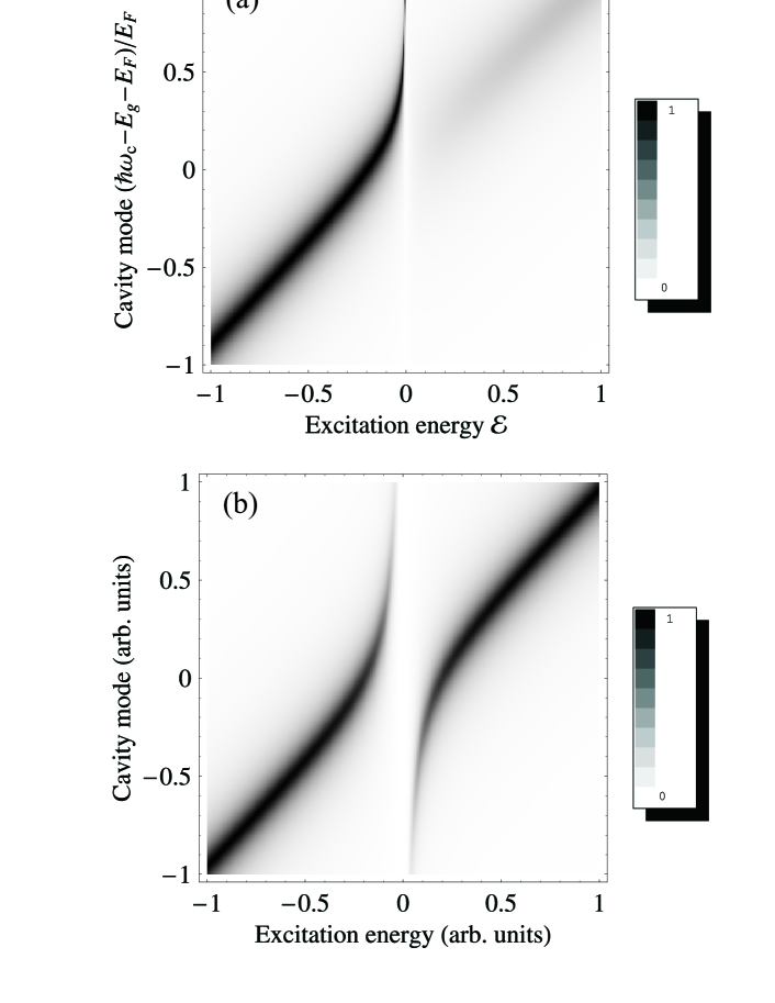
Figure 2: (Color online). Quantum microcavity transmission coefficient $|t_{qmc}|^{2}$ [Eq. (11)] as a function of the excitation energy $\mathcal{E}=(\hbar\omega-E_{g}-E_{F})/E_{F}$ and the cavity mode energy $(\hbar\omega_{c}-E_{F})/E_{F}$. (a) and (b) are the surface plots (the gray-level scale is shown to the right) corresponding to the Mahan singularity and discrete excitonic state, respectively. (c), (d) and (e) are the horizontal cuts of the panel (a) for different cavity mode energies $(\hbar\omega_{c}-E_{F})/E_{F}=-1$, $0$ and $1$, from the top to the bottom. The parameters used are: $\delta=0.63$, $\mathcal{C}=0.1$, $R=0.98$.

Figure 2 presents the microcavity transmission coefficient $|t_{qmc}|^{2}$ calculated as a function of excitation energy and cavity mode position. The maximum of the transmission coefficient [dark area of Fig. 2(a)] corresponds to the eigenmodes of the quantum microcavity. They can be found analytically as zeros of the denominator in Eq. (11):

$$\mathcal{D}=[r_{m}(2r+1)e^{\mathrm{i}\psi_{b}}-1](r_{m}e^{\mathrm{i}\psi_{b}}+1).$$ (12)

The second factor in Eq. (12) corresponds to the cavity modes which are not coupled to the two-dimensional electron gas. The first factor describes new (polaritonic) modes arising due to the light-matter interaction. Assuming that the relevant frequencies lie in the vicinity of the stop-band center of Bragg mirror one may use the following approximate expressions for the Bragg mirror reflection and transmission coefficients Kavokin and Malpuech (2003); Panzarini et al. (1999); Ivchenko (2005)

$$r_{m}=\sqrt{R}e^{\mathrm{i}\psi_{m}(\omega)},\qquad t_{m}=\pm\mathrm{i}r_{m}\sqrt{(1-R)/R}.$$ (13)

Here $R$ is the intensity reflection coefficient and $\psi_{m}(\omega)$ is a phase. In the vicinity of the stop-band center it is a linear function of $\omega$. Panzarini et al. (1999) Eq. (12) clearly shows that the only independent phase parameter is $\psi=\psi_{m}+\psi_{b}$, which can be recast in form $\psi=(\omega-\omega_{c})/\bar{\omega}$, where $\omega_{c}$ is the cavity resonance frequency, and $c/\bar{\omega}=(L_{DBR}+L_{b})n_{b}$ is the effective cavity length (including the active layer length, $L_{b}$, and the mirror penetration length, $L_{DBR}$) Kavokin and Malpuech (2003). Substituting Eq. (13) into the first factor of Eq. (12) under assumption that $(\omega-\omega_{c})/\bar{\omega}\ll 1$ and $R\to 1$ we arrive to

$$\omega_{c}-\omega=2Q\bar{\omega}G(\omega).$$ (14)

It is convenient to introduce the dimensionless coupling constant $\mathcal{C}=mQ\bar{\omega}/(\pi\hbar E_{F})$, which can be related to the coupling constant $V_{R}$ of the undoped cavity as $\mathcal{C}=(k_{F}a_{B}V_{R})^{2}/32E_{F}^{2}$.

Equation (14) has a very transparent physical meaning: it describes the linear coupling between the microcavity photon and the continuum of states of all electron-hole pair exciations. It is equivalent to the eigenenergy equation for the following Hamiltonian

$$\mathcal{H}=\hbar\omega_{c}c^{\dagger}c+\sum_{\bm{k}}\left(E_{g}+\frac{\hbar^{2}k^{2}}{2m}\right)a_{\bm{k}}^{\dagger}a_{\bm{k}}+$$ (15)

$$\sqrt{\frac{2Q\bar{\omega}\hbar}{\mathcal{S}}}\sum_{\bm{k}}\left|\frac{M_{k}}{M_{k}^{0}}\right|^{2}[1-n_{F}(k)](c^{\dagger}a_{\bm{k}}+ca^{\dagger}_{\bm{k}}),$$

where $c^{\dagger}$, $c$ are the creation (annihilation) operators for the cavity photon and $a_{\bm{k}}^{\dagger}$, $a_{\bm{k}}$ are the creation (annihilation) operators for electron-hole pair excitations. Thus, the description of the light matter interaction in the doped system is reduced to the quantum mechanical problem of the interaction between the discrete state and a continuum. suris

The graphical solution of Eq. (14) is represented in Fig. 1. The dotted line shows the left-hand side of Eq. (14) and the blue solid line shows the right hand side. All the states with $\hbar\omega\geq E_{g}+E_{F}$ belong to continuum. Thus, non-trivial solutions of Eq (14) can be for $\hbar\omega<E_{g}+E_{F}$ only. One may identify two regimes of light-matter coupling depending on the number of solutions of Eq. (14).

In the first case, the discrete state with an energy $\hbar\omega_{0}$ exists for all the values of $\hbar\omega$, i.e. $G(\omega)$ diverges for $\hbar\omega=E_{g}+E_{F}$. This is the case of the Mahan singularity in the optical absorbtion, Eq. (5), or of the undoped two-dimensional system. In the second regime, where $G[(E_{g}+E_{F})/\hbar]$ is finite, the discrete state exists only for $\hbar\omega_{c}<\hbar\omega_{m}$, where the limiting frequency $\omega_{m}=E_{g}+E_{F}+2Q\bar{\omega}G[(E_{g}+E_{F})/\hbar]$. This case can be realized if the ‘optical’ density of states $\propto|M_{k}|^{2}$ is zero at the threshold as it takes place for an undoped crystal in the vicinity of the fundamental absorbtion edge or for $\delta<0$, corresponding to the dominant contribution of the orthogonality catastrophe, Eq. (6).

In other words, with an increase of the cavity mode frequency $\omega_{c}$ the photon state repels from the continuum due to the light-matter interaction, but depending on the coupling strength it can either be pushed away from the continuum or can merge a continuum. It is illustrated in Fig. 2(a): as the cavity mode position shifts to higher energies, the energy corresponding to the maximum of transmission increases and approaches the singularity position $\hbar\omega=E_{g}+E_{F}$. The strong repulsion of the photonic state from the continuum is seen; in our case of singular susceptibility ($\delta>0$) the discrete photonic states survives for any cavity mode position, see panels (c)–(e). This discrete photonic state peak becomes narrower for larger $\hbar\omega_{c}$ [it is most pronounced in Fig. 2(e)] but the allowance for the inhomogeneous broadening of the Mahan singularity will smear this peak. Due to an enhanced absorbtion at $\hbar\omega>E_{g}+E_{F}$ the transmission tends to zero at $\hbar\omega$ approaching to $E_{g}+E_{F}$ from high-energy side. An additional maximum in transmission appears at $\hbar\omega>E_{g}+E_{F}$ at the energy approximately equal to bare cavity mode position $\hbar\omega_{c}$ becoming more pronounced with an increase of cavity mode energy. It can be attributed to the resonant state formed by the cavity mode ‘inside’ the continuum of electron-hole excitations and corresponds to the third intersection of the solid and dotted curves in Fig. 1, see next section.

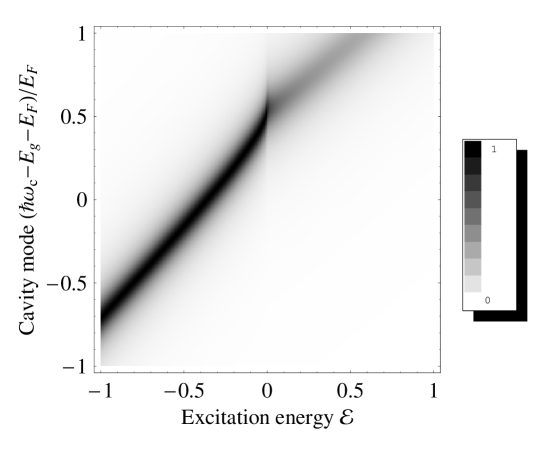
Figure 3: Quantum microcavity transmission coefficient $|t_{qmc}|^{2}$ [Eq. (11)] as a function of the excitation energy $\mathcal{E}=(\hbar\omega-E_{g}-E_{F})/E_{F}$ and the cavity mode energy $(\hbar\omega_{c}-E_{F})/E_{F}$ calculated for the case of absent singularity. The parameters used are: $\delta=-0.63$, $\mathcal{C}=0.1$, $R=0.98$.

For the smaller but non-negative values of $\delta$ the calculated transmission spectra are qualitatively the same. The decrease of $\delta$ leads to the sharper peak with larger wings of susceptibility’s real part. It results in less pronounced discrete state and smaller spacing between absorbtion edge and the last transmission maximum.

The case of the negative $\delta$ is presented in Fig. 3. In this case the discrete ‘dressed’ photonic state survives only up to $\omega_{c}=\omega_{m}$. The behaviour of the transmission maximum reflects the real part of susceptibility and a peak is seen in the vicinity of the absorbtion edge. The absorbtion above the edge is smaller as compared to the case of $\delta>0$ thus resonant states inside the continuum are more pronounced.

This situation depicted in Figs. 2(a), 3 is qualitatively different from that observed in undoped cavities tuned to the vicinity of exciton resonance, see Fig. 2(b). In this case cavity photon and exciton can be described as two oscillators. Their coupling leads to the repulsion and anticrossing of the levels, in the strong coupling regime two discrete states (polaritons) corresponding to the maxima of the transmission are present.

IV Time-resolved emission

The light-matter interaction manifests itself in the time resolved experiments as well. Consider an experiment where the bare photon mode is excited by a short pulse and the emission intensity is analyzed. In the case of the undoped quantum well and a microcavity tuned to the exciton resonance this intensity demonstrates the quantum beats, corresponding to the energy transfer between the photon and exciton states. rabi In the case of doped system the photon interacts with a continuum of states and the time-domain response is drastically different.

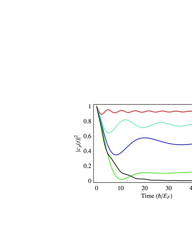
Figure 4: (Color online). The photon intensity $|c_{p}(t)|^{2}$ as a function of time calculated according to Eq. (18). Different curves correspond to different cavity mode energies $(\hbar\omega_{c}-E_{F})/E_{F}=-1$, $-0.25$, $0$, $0.5$ and $1$ (curves 1–5, respectively). The parameters used are: $\delta=0.63$, $\mathcal{C}=0.1$.

In order to find the time-resolved emission from the microcavity containing a doped quantum well we solve Schroedinger equation with Hamiltoninan (15) and represent the wavefunction of the system as

$$\Psi(t)=\left[c_{p}(t)c^{\dagger}+\sum_{\bm{k}}c_{\bm{k}}(t)a^{\dagger}_{\bm{k}}\right]|0\rangle.$$ (16)

Here $|0\rangle$ is the ‘vacuum state’, $c_{p}(t)$ and $c_{\bm{k}}(t)$ are time-dependent coefficients of the photon and continuums states. Substituting Eq. (16) into the temporal Schroedinger equation

$$\mathrm{i}\hbar\frac{\partial\Psi(t)}{\partial t}=\mathcal{H}\Psi(t),$$

one arrives to the system of linear coupled equations for the functions $c_{p}(t)$, $c_{\bm{k}}(t)$. It can be solved by Laplace transformation.

We consider the most interesting case of the initial excitation of the bare photon mode $[c_{p}(0)=1]$ and analyze the time dependence $c_{p}(t)$ which corresponds to the photon fraction of the polaritonic mode (i.e. quantum microcavity emission amplitude):

$$c_{p}(t)=\int_{\gamma-\mathrm{i}\infty}^{\gamma+\mathrm{i}\infty}\frac{e^{st}}{s+\mathrm{i}\omega_{c}-2\mathrm{i}Q\bar{\omega}G(\mathrm{i}\hbar s)}\frac{\mathrm{d}\hbar s}{2\pi\mathrm{i}},$$ (17)

where $\gamma$ is sufficiently large real number. We note that $\mathrm{i}0$ term in the denominator of $G(\omega)$ should be omitted in Eq. (17).

This integral can be calculated by the standard procedure. kyrola Note that the subintegral expression has following singularities. First, there may be a pole for the imaginary $s=-\mathrm{i}\omega_{0}$, there $\omega=\omega_{0}$ satisfies the bound-state equation (14) which corresponds to the discrete state. Second, there is a branch-cut along the positive part of the imaginary axis $E_{g}+E_{F}\leq-\mathrm{i}s$ which corresponds to the contribution of the continuum. As a result, integral (17) is recast in a form

$$c_{p}(t)=\mathop{\rm res}_{\omega=\omega_{0}}{\frac{e^{-\mathrm{i}\omega_{0}t}}{\omega-\omega_{c}+2Q\bar{\omega}G(\omega)}}+$$ (18)

$$\int_{E_{g}+E_{F}}^{\infty}\frac{e^{-\mathrm{i}\tilde{s}t}\alpha^{2}(\hbar\tilde{s})\mathrm{d}\hbar\tilde{s}}{\left[\hbar\tilde{s}-\hbar\omega_{c}+vp\int_{E_{g}+E_{F}}^{\infty}\frac{\alpha^{2}(E)}{E-\hbar\tilde{s}}\mathrm{d}E\right]^{2}+\pi^{2}\alpha^{4}(\tilde{s})},$$

where

$$\alpha(E)=\frac{mQ\bar{\omega}}{\pi\hbar^{2}}\left|\frac{M_{k}}{M_{k}^{0}}\right|^{2},\quad k=\sqrt{\frac{2m(E-E_{g})}{\hbar^{2}}}.$$

This result can be interpreted in the terms of eigenmodes of the system. The first term in Eq. (18) corresponds to the discrete state (i.e. “dressed photon”) contribution, while the second term describes the effects of the continuum. Initially excited bare photonic mode is divided among new eigenmodes: discrete state (if it exists) and a continuum. The part corresponding to the discrete state survives, while that of continuum is spread over all possible energies. The main contribution to the second term of Eq. (18) comes from the points $\tilde{s}_{i}$ where the subintegral expression has a sharp maximum (i.e. to the intersection points for $\mathcal{E}>0$ in Fig. 1). In a crude approximation each of such contributions reads

$$\exp{[-\mathrm{i}\tilde{s}_{i}t-\alpha^{2}(\hbar\tilde{s}_{i})\hbar^{-1}t]},$$

thus it can be considered as a quasi-bound state (or resonance). The microcavity emission $\propto|c_{p}(t)|^{2}$ will demonstrate the decaying quantum beats between the discrete state (dressed photon) and the continuum (resonances),

$$|c_{p}(t)|^{2}\propto\sum_{i}\cos{[(\omega_{0}-\tilde{s}_{i})t+\varphi_{i}]}\exp{[-\alpha^{2}(\hbar\tilde{s}_{i})\hbar^{-1}t]},$$ (19)

where $\varphi_{i}$ are the initial phases of the beats.

Fig. 4 shows the results of numerical integration in Eq. (18). The decaying beats are observed. The beats frequency is a non-monotonous function of detuning: it decreases as $\hbar\omega_{c}$ approaches $E_{g}+E_{F}$ from below (as the main contribution to beats are given by the first resonance near the Mahan singularity, see first intersection point in Fig. 1), reaches a minimum at $\hbar\omega_{c}\approx E_{g}+E_{F}$ and then increases, as the energy separation between the discrete state (with energy close to $E_{g}+E_{F}$) and the second resonance increases. The damping of the beats results from the non-commensurability of the continuum frequencies.

In this treatment we have disregarded the photon leakage through the Bragg mirrors and inhomogeneous broadening of the Fermi-edge singularity. Both of these effects give rise to an additional damping of the beats as well as to the overall decay of $c_{p}(t)$.

The time-domain response of the microcavity in the case where the singularity is absent, $\delta<0$ in Eq. (1) is qualitatively the same. In the case of $\omega_{c}<\omega_{m}$ the real discrete photonic state exists and the emission intensity is similar to that presented in Fig. 4. For $\omega_{c}>\omega_{m}$ only contribution of continuum remains and $c_{p}(t)$ decays to zero even without photon leakage through the mirrors and inhomogeneous broadening.

V Conclusions

To conclude, we have theoretically studied the light-matter coupling in the microcavities containing doped quantum wells. In such structures the cavity photon interacts with the continuum of the electron-hole pair excitations. The new eigenmodes of the system are the discrete state (corresponding to the ‘dressed’ cavity photon) and the continuum of electron-hole pairs modified by the interaction with the cavity photon. We have analyzed the effects of the ‘optical’ density of states on the bound state formation. It was shown that the step-like or singular behavior of the absorbtion coefficient at the threshold implies the bound state presence for any detuning between the cavity mode and the threshold energy. If the optical density of states is non-singular at the threshold, the bound photonic state survives only up to some limiting detuning. We have investigated the reflection and transmission spectra of the doped microcavities and shown that they are qualitatively different from those obtained in the undoped case where discrete excitonic state is coupled to the discrete photonic state. The time domain response of the doped microcavity is shown to demonstrate the damped beats revealing the energy transfer between the discrete state and the continuum and the energy spread in the continuum.

- (1) C. Weisbuch, M. Nishioka, A. Ishikawa, and Y. Arakawa, Phys. Rev. Lett. 69, 3314 (1992).
- Kavokin and Malpuech (2003) A. Kavokin and G. Malpuech, Cavity Polaritons, vol. 32 of Thin Films and Nanostructures (Elsevier, 2003).
- (3) Deveaud, Benoit (Ed.) The Physics of Semiconductor Microcavities From Fundamentals to Nanoscale Devices, Wiley-VCH (2006).
- (4) S. Jiang, S. Machida, Y. Takiguchi, and Y. Yamamoto, Appl. Phys. Lett. 73, 3031 (1998).
- (5) D. Bajoni, M. Perrin, P. Senellart, A. Lematre, B. Sermage, and J. Bloch, Phys. Rev. B 73, 205344 (2006).
- Qarry et al. (2003) A. Qarry, R. Rapaport, G. Ramon, E. Cohen, A. Ron, and L. N. Pfeiffer, Semicond. Sci. and Tech. 18, S331 (2003).
- Mahan (1967a) G. D. Mahan, Phys. Rev. 153, 882 (1967a); G. D. Mahan, Phys. Rev. 163, 612 (1967b).
- ROULET et al. (1969) B. Roulet, J. Gavoret, and P. Nozières, Phys. Rev. 178, 1072 (1969).
- Hawrylak (1991) P. Hawrylak, Phys. Rev. B 44, 3821 (1991).
- Pardee and Mahan (1973) W. J. Pardee and G. D. Mahan, Phys. Lett. A 45, 117 (1973).
- Penn et al. (1981) D. R. Penn, S. M. Girvin, and G. D. Mahan, Phys. Rev. B 24, 6971 (1981).
- (12) P. W. Anderson, Phys. Rev. Lett. 18, 1049 (1967).
- Andreani et al. (1991) L. C. Andreani, F. Tassone, and F. Bassani, Solid State Commun. 77, 641 (1991).
- Ivchenko (2005) E. L. Ivchenko, Optical Spectroscopy of Semiconductor Nanostructures (Alpha Science, 2005).
- (15) E.L. Ivchenko, G.E. Pikus, Superlattices and Other Heterostructures, (Springer, 2nd ed., 1997).
- Panzarini et al. (1999) G. Panzarini, L. C. Andreani, A. Armitage, D. Baxter, M. S. Skolnick, V. N. Astratov, J. S. Roberts, A. V. Kavokin, M. R. Vladimirova, and M.A.Kaliteevski, Fiz. Tverd. Tela 41, 1337 (1999).
- (17) For review see S. M. Kogan and R. A. Suris, Zh. Eksp. Teor. Fiz. 50, 1279 (1966) [Sov. Phys. JETP 23, 850 (1966)]; I. B. Levinson and E. I. Rashba, Usp. Fiz. Nauk 111, 683 (1973) [Sov. Phys. Usp. 16, 892 (1973)].
- (18) E. Kyrölä, J. Phys. B: At. Mol. Phys. 19, 1437 (1986).