Mixtures of ultracold fermions with unequal masses

Abstract

We analyze the phase diagram of superfluidity for two-species fermion mixtures from the Bardeen-Cooper-Schrieffer (BCS) to Bose-Einstein condensation (BEC) limit as a function of scattering parameter, population imbalance and mass anisotropy. We identify regions corresponding to normal, or uniform/non-uniform superfluid phases, and discuss topological quantum phase transitions in the BCS, unitarity and BEC limits. We derive the Ginzburg-Landau equation near the critical temperature, and show that it describes a dilute mixture of paired and unpaired fermions in the BEC limit. We also obtain the zero temperature low frequency and long wavelength collective excitation spectrum, and recover the Bogoliubov relation for weakly interacting dilute bosons in the BEC limit. Lastly, we discuss the effects of harmonic traps and the resulting density profiles in the BEC regime.

I Introduction

The evolution from Bardeen-Cooper-Schrieffer (BCS) state to Bose-Einstein condensation (BEC) is an important topic of current research for condensed matter, nuclear, atomic and molecular physics communities. Recent advances in atomic physics have allowed for the study of superfluid properties in symmetric two-component fermion superfluids (equal mass and equal populations) as a function of scattering length, where the theoretically predicted crossover from BCS to BEC was observed leggett ; nsr ; carlos .

Since the population of each component as well as the interaction strength between two components are experimentally tunable, these knobs enabled the study of the BCS to BEC evolution in asymmetric two-component fermion superfluids (equal mass but unequal populations) mit ; rice . In contrast with the crossover physics found in the symmetric case, these experiments have demonstrated the existence of phase transitions between normal and superfluid phases, as well as phase separation between superfluid (paired) and normal (excess) fermions as a function of population imbalance  liu ; yip-stability ; bedaque ; carlson ; pao ; son ; sheehy ; ho ; bulgac ; cheng ; machida ; pieri ; torma ; yi ; chevy ; silva ; haque .

Arguably one of the next frontiers of exploration in cold Fermi gases is the study of asymmetric two-component fermion superfluidity (unequal masses and equal or unequal populations) in two-species fermion mixtures from the BCS to the BEC limit. Earlier works on two-species fermion mixtures were limited to the BCS regime liu ; yip-stability ; bedaque ; lianyi . However, very recently, the evolution from BCS to BEC was preliminarily addressed in homogenous systems as a function of population imbalance and scattering length especially for ⁶Li and ⁴⁰K mixture and also for other mixtures including ⁶Li and ⁸⁷Sr and ⁴⁰K and ⁸⁷Sr mixtures iskin-mixture ; iskin-mixture2 ; parish . In addition, the superfluid phase diagram of trapped systems at unitarity was also analyzed as a function of population imbalance and mass anisotropy pao-mixture .

In this manuscript, we study the BCS to BEC evolution of asymmetric two-component fermion superfluids as a function of population imbalance and mass anisotropy, and extend our previous works iskin-mixture ; iskin-mixture2 in this area. Our main results are as follows. For a homogeneous system, we analyze the zero temperature phase diagram for ultra cold fermion mixtures as a function of mass anisotropy and population imbalance. We identify regions corresponding to normal, uniform or non-uniform superfluid phases, and discuss topological quantum phase transitions in the BCS, unitarity and BEC limits. We derive the Ginzburg-Landau theory near the critical temperature, and show that it describes a dilute mixture of weakly interacting paired and unpaired fermions in the BEC limit. We also derive the zero temperature low frequency and long wavelength collective excitation spectrum for zero population imbalance, and recover the Bogoliubov relation for weakly interacting dilute bosons in the BEC limit. In addition, we describe analytically the phase separation boundaries of the resulting Bose-Fermi mixture of paired fermions and unpaired fermions in the BEC limit. Lastly, we discuss the effects of harmonic traps and the resulting density profiles of paired and unpaired fermions in the BEC regime.

The rest of the paper is organized as follows. In Sec. II, we introduce the imaginary-time functional integration formalism, and obtain the self-consistency (order parameter and number) equations. In Sec. III, we discuss the evolution from BCS to BEC superfluidity at zero temperature within the saddle point approximation, and we analyze the order parameter, chemical potential, and stability of the saddle-point solutions. In Sec. IV, we discuss gaussian fluctuations near the critical temperature, and we obtain the low energy collective excitations and corrections to the saddle point phase diagram in the BEC region at zero temperature. In addition, we discuss the effects of harmonic traps on the density profile of paired and unpaired fermions at zero temperature. A summary of our conclusions is given in Sec. V. Lastly, we present in Appendices A, B, and C the elements of the inverse fluctuation matrix, and their low frequency and long wavelength expansion coefficients at finite and zero temperatures.

II Functional Integral Formalism

To describe a dilute two-species Fermi gas in three dimensions, we start from the Hamiltonian ($\hbar=1$)

$$H=\sum_{\mathbf{k},\sigma}\xi_{\mathbf{k},\sigma}a_{\mathbf{k},\sigma}^{\dagger}a_{\mathbf{k},\sigma}+\sum_{\mathbf{k},\mathbf{k^{\prime}},\mathbf{q}}U(\mathbf{k},\mathbf{k^{\prime}})b_{\mathbf{k},\mathbf{q}}^{\dagger}b_{\mathbf{k^{\prime}},\mathbf{q}},$$ (1)

where the pseudo-spin $\sigma$ labels both the type and hyperfine states of atoms represented by the creation operator $a_{\mathbf{k},\sigma}^{\dagger}$, and $b_{\mathbf{k},\mathbf{q}}^{\dagger}=a_{\mathbf{k}+\mathbf{q}/2,\uparrow}^{\dagger}a_{-\mathbf{k}+\mathbf{q}/2,\downarrow}^{\dagger}$. Here, $\xi_{\mathbf{k},\sigma}=\epsilon_{\mathbf{k},\sigma}-\mu_{\sigma}$, where $\epsilon_{\mathbf{k},\sigma}=k^{2}/(2m_{\sigma})$ is the energy and $\mu_{\sigma}$ is the chemical potential of the fermions. Notice that we allow for the fermions to have different masses $m_{\sigma}$ and different populations controlled by independent chemical potentials $\mu_{\sigma}$. The attractive fermion-fermion interaction $U(\mathbf{k},\mathbf{k^{\prime}})$ can be written in a separable form as $U(\mathbf{k},\mathbf{k^{\prime}})=-g\Gamma^{*}_{\mathbf{k}}\Gamma_{\mathbf{k^{\prime}}}$ where $g>0$, and $\Gamma_{\mathbf{k}}=1$ for the zero-range s-wave contact interaction considered in this manuscript.

II.1 Effective action

The gaussian effective action for $H$ is

$$S_{\rm Gauss}=S_{0}+\frac{\beta}{2}\sum_{q}\bar{\Lambda}^{\dagger}(q)\mathbf{F}^{-1}(q)\bar{\Lambda}(q),$$ (2)

where $\beta=1/T$ and $q=(\mathbf{q},v_{\ell})$ with bosonic Matsubara frequency $v_{\ell}=2\ell\pi/\beta$. Here, the saddle point action is given by

$$S_{0}=\beta\frac{|\Delta_{0}|^{2}}{g}-\sum_{p}\rm{Tr}\ln[\mathbf{G}^{\rm sp}(p)/\beta]^{-1},$$ (3)

where $p=(\mathbf{k},w_{\ell})$ with fermionic Matsubara frequency $w_{\ell}=(2\ell+1)\pi/\beta$, $\Delta_{\mathbf{k}}=\Delta_{0}\Gamma_{\mathbf{k}}$ is the order parameter, and $(\mathbf{G}^{\rm sp})^{-1}(p)$ is the inverse fermion propagator. The matrix $(\mathbf{G}^{\rm sp})^{-1}(p)$ is defined by

$$(\mathbf{G}^{\rm sp})^{-1}(p)=\left(\begin{array}[]{cc}iw_{\ell}-\xi_{\mathbf{k},\uparrow}&\Delta_{\mathbf{k}}\\ \Delta_{\mathbf{k}}^{*}&iw_{\ell}+\xi_{\mathbf{k},\downarrow}\end{array}\right).$$ (4)

Furthermore, the vector $\bar{\Lambda}^{\dagger}(q)$ is the order parameter fluctuation field and $\mathbf{F}^{-1}(q)$ is the inverse fluctuation propagator. The matrix elements of $\mathbf{F}^{-1}(q)$ are given by

$$\mathbf{F}^{-1}_{1,1}(q) = \frac{V}{g}-\frac{1}{\beta}\sum_{p}\mathbf{G}^{\rm sp}_{\uparrow,\uparrow}(\frac{q}{2}+p)\mathbf{G}^{\rm sp}_{\downarrow,\downarrow}(\frac{q}{2}-p)|\Gamma_{\mathbf{k}}|^{2},$$ (5)

$$\mathbf{F}^{-1}_{1,2}(q) = \frac{1}{\beta}\sum_{p}\mathbf{G}^{\rm sp}_{\uparrow,\downarrow}(\frac{q}{2}+p)\mathbf{G}^{\rm sp}_{\uparrow,\downarrow}(\frac{q}{2}-p)|\Gamma_{\mathbf{k}}|^{2}.$$ (6)

Notice that $\mathbf{F}^{-1}_{2,1}(q)=(\mathbf{F}^{-1}_{1,2})^{*}(q)$ and $\mathbf{F}^{-1}_{2,2}(q)=\mathbf{F}^{-1}_{1,1}(-q)$. These matrix elements are described further in appendix A. The fluctuation term in the action leads to a correction to the thermodynamic potential, which can be written as $\Omega_{{\rm Gauss}}=\Omega_{0}+\Omega_{{\rm fluct}}$ with $\Omega_{0}=S_{0}/\beta$ and $\Omega_{{\rm fluct}}=(1/\beta)\sum_{q}\ln\det[\mathbf{F}^{-1}(q)/\beta]$. Next, we derive the self-consistency equations.

II.2 Self-consistency equations

The saddle point condition $\delta S_{0}/\delta\Delta_{0}^{*}=0$ or the relation

$$\Delta_{\mathbf{k^{\prime}}}=-\frac{1}{\beta}\lim_{\tau\to 0}\sum_{p}U(\mathbf{k},\mathbf{k^{\prime}})\mathbf{G}^{\rm sp}_{\uparrow,\downarrow}(p)\exp(iw_{\ell}\tau)$$ (7)

leads to an equation for the order parameter

$$\frac{1}{g}=\sum_{\mathbf{k}}\frac{|\Gamma_{\mathbf{k}}|^{2}}{2E_{\mathbf{k},+}}{\cal X}_{\mathbf{k},+},$$ (8)

where ${\cal X}_{\mathbf{k},\pm}=({\cal X}_{\mathbf{k},1}\pm{\cal X}_{\mathbf{k},2})/2$ with ${\cal X}_{\mathbf{k},s}=\tanh(\beta E_{\mathbf{k},s}/2).$ Notice that, at low temperatures $T\approx 0$, $\theta(-E_{\mathbf{k,s}})=\lim_{\beta\to\infty}{\cal X}_{\mathbf{k},s}$, where $\theta(x)$ is the Heaviside function. Here, $E_{\mathbf{k},\pm}=(E_{\mathbf{k},1}\pm E_{\mathbf{k},2})/2$ and $\xi_{\mathbf{k},\pm}=(\xi_{\mathbf{k},\uparrow}\pm\xi_{\mathbf{k},\downarrow})/2=k^{2}/(2m_{\pm})-\mu_{\pm},$ where

$$E_{\mathbf{k},1} = (\xi_{\mathbf{k},+}^{2}+|\Delta_{\mathbf{k}}|^{2})^{1/2}+\xi_{\mathbf{k},-},$$ (9)

$$E_{\mathbf{k},2} = (\xi_{\mathbf{k},+}^{2}+|\Delta_{\mathbf{k}}|^{2})^{1/2}-\xi_{\mathbf{k},-}$$ (10)

are the quasiparticle and negative of the quasihole energies respectively, $m_{\pm}=2m_{\uparrow}m_{\downarrow}/(m_{\downarrow}\pm m_{\uparrow})$ and $\mu_{\pm}=(\mu_{\uparrow}\pm\mu_{\downarrow})/2.$ Notice that $m_{+}$ is twice the reduced mass of the $\uparrow$ and $\downarrow$ fermions, and that the equal mass case corresponds to $|m_{-}|\to\infty$. As usual, we eliminate $g$ in favor of the scattering length $a_{F}$ via the relation

$$\frac{1}{g}=-\frac{m_{+}V}{4\pi a_{F}}+\sum_{\mathbf{k}}\frac{|\Gamma_{\mathbf{k}}|^{2}}{2\epsilon_{\mathbf{k},+}},$$ (11)

where $\epsilon_{\mathbf{k},\pm}=(\epsilon_{\mathbf{k},\uparrow}\pm\epsilon_{\mathbf{k},\downarrow})/2.$

The order parameter equation has to be solved self-consistently with number equations $N_{\sigma}=-\partial\Omega/\partial{\mu_{\sigma}}$ which have two contributions $N_{\sigma}=N_{0,\sigma}+N_{{\rm fluct},\sigma}$. The first term $N_{0,\sigma}=-\partial\Omega_{0}/\partial{\mu_{\sigma}}$ or the relation

$$N_{0,\sigma}=\frac{\gamma_{\sigma}}{\beta}\lim_{\tau\to 0}\sum_{p}\mathbf{G}^{\rm sp}_{\sigma,\sigma}(p)\exp(i\gamma_{\sigma}w_{\ell}\tau)$$ (12)

leads to the saddle point contribution, and is given by

$$N_{0,\sigma}=\sum_{\mathbf{k}}\left(\frac{1-\gamma_{\sigma}{\cal X}_{\mathbf{k},-}}{2}-\frac{\xi_{\mathbf{k},+}}{2E_{\mathbf{k},+}}{\cal X}_{\mathbf{k},+}\right).$$ (13)

Here, $\gamma_{\uparrow}=+1$ and $\gamma_{\downarrow}=-1$. Similarly, the second term $N_{{\rm fluct},\sigma}=-\partial\Omega_{{\rm fluct}}/\partial{\mu_{\sigma}}$ leads to the fluctuation contribution, and is given by

$$N_{{\rm fluct},\sigma}=-\frac{1}{\beta}\sum_{q}\frac{\partial[\det\mathbf{F}^{-1}(q)]/\partial{\mu_{\sigma}}}{\det\mathbf{F}^{-1}(q)}.$$ (14)

While the saddle point contribution is sufficient for a semi-quantitative analysis at zero temperature ($T\approx 0$), inclusion of the fluctuation contribution is necessary to recover BEC physics at finite temperatures ($T\to T_{c}$).

When populations of the pseudo-spin components are balanced ($N_{\uparrow}=N_{\downarrow}$), the results for $|\Delta_{0}|$ and $\mu_{+}$ ($\mu_{-}$ is irrelevant in this case) of $m_{\uparrow}\neq m_{\downarrow}$ case can be obtained from the results for $|\Delta_{0}|$ and $\mu$ of $m=m_{\uparrow}=m_{\downarrow}$ case via a substitution of $m\to m_{+}$. However, when populations of the pseudo-spin components are imbalanced ($N_{\uparrow}\neq N_{\downarrow}$), we need to solve all three self-consistency equations, since population imbalance is achieved when either $E_{\mathbf{k},1}$ or $E_{\mathbf{k},2}$ is negative in some regions of momentum space, which is discussed next.

III Saddle point results

At low temperatures $T\approx 0$, the saddle point self-consistency (order parameter and number) equations are sufficient to describe the evolution of superfluidity from the BCS to the BEC limit. In this section, we analyze amplitude of the order parameter $|\Delta_{0}|$ and chemical potentials $\mu_{\sigma}$ as a function of mass anisotropy $m_{r}=m_{\uparrow}/m_{\downarrow}$ and population imbalance $P=N_{-}/N_{+}$ for a set of fixed scattering parameters $1/(k_{F,+}a_{F})$. Here $N_{\pm}=(N_{\uparrow}\pm N_{\downarrow})/2$ and $k_{F,\pm}^{3}=(k_{F,\uparrow}^{3}\pm k_{F,\downarrow}^{3})/2$. Because of the parabolic dispersion relation, the density of $\uparrow$ fermions is $n_{\uparrow}=k_{F,{\uparrow}}^{3}/(6\pi^{2})$ and the density of $\downarrow$ fermions is $N_{\downarrow}=k_{F,{\downarrow}}^{3}/(6\pi^{2})$. Here, the Fermi momenta $k_{F,{\uparrow}}$ and $k_{F,{\downarrow}}$ are determined from the Fermi energies $\epsilon_{F,\sigma}=k_{F,\sigma}^{2}/(2m_{\sigma})$. Therefore, the total fermion density is

$$n=n_{\uparrow}+n_{\downarrow}=\frac{k_{F,+}^{3}}{3\pi^{2}}.$$ (15)

Using the notations described in the preceding paragraph, we can solve the self-consistency Eqs. (8), (11) and (13). For instance, in Fig. 1, we show self-consistent solutions of $|\Delta_{0}|$, $\mu_{+}$ and $\mu_{-}$ (in units of $\epsilon_{F,+}$) as a function of $m_{r}$ when $P=0.5$ and $1/(k_{F,+}a_{F})=0$. Here, $\epsilon_{\rm F,\pm}=k_{F,\pm}^{2}/(2m_{\pm})$. With increasing mass anisotropy (or decreasing $m_{r}$), we find that both $|\Delta_{0}|$ and $\mu_{+}$ increase until $m_{r}\approx 0.4$. However, further decrease in $m_{r}$ beyond $m_{r}\approx 0.4$ leads to a saturation of both $|\Delta_{0}|$ and $\mu_{+}$ with a small cusp in both quantities. The cusp is best seen in Fig. 1 at small grazing angles. Therefore, the evolution from $m_{r}=1$ to $m_{r}\to 0$ is non-analytic when $m_{r}\approx 0.4$, and the evolution is not a crossover. These cusps in $|\Delta_{0}|$ and $\mu_{+}$ are more pronounced for higher $|P|$, and they signal a topological quantum phase transition discussed below. Notice that, for $P=0$, the evolution of $|\Delta_{0}|$ and $\mu_{+}$ is analytic for all $m_{r}$, and the evolution is just a crossover.

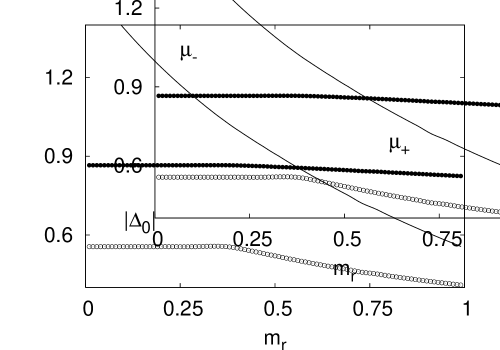
Figure 1: Plots of $|\Delta_{0}|$, $\mu_{+}$ and $\mu_{-}$ (in units of $\epsilon_{F,+}$) as a function of $m_{r}$, when $P=0.5$ and $1/(k_{F,+}a_{F})=0$ (unitarity limit). Notice the presence of small cusps in $|\Delta_{0}|$ and $\mu_{+}$ when $m_{r}\approx 0.4$ which signal a topological quantum phase transition discussed below. These cusps are more pronounced for higher $|P|$ (not shown), but are best seen in this figure at small grazing angles.

Next, we discuss the stability of uniform superfluidity using two criteria  pao ; gubankova ; lianyi2 ; sheehy2 ; pao-stability : positive definite compressibility $\mathbf{\kappa}(T)$ and superfluid density $\mathbf{\rho}(T)$ matrices.

III.1 Stability of uniform superfluidity

In order to analyze the phase diagram at $T=0$, we solve the saddle point self-consistency (order parameter and number) equations for all $P$ and $m_{r}$ for a set of $1/(k_{F,+}a_{F})$, and check the stability of saddle point solutions for the uniform superfluid phase using two criteria.

The first criterion requires that the compressibility matrix $\mathbf{\kappa}(T)$ is positive definite, where the elements of $\mathbf{\kappa}(T)$ are $\kappa_{\sigma,\sigma^{\prime}}(T)=-\partial^{2}\Omega_{0}/(\partial\mu_{\sigma}\partial\mu_{\sigma^{\prime}}).$ This criterion is related (identical) to the condition that the curvature

$$\frac{\partial^{2}\Omega_{0}}{\partial\Delta_{0}^{2}}=\sum_{\mathbf{k}}|\Delta_{\mathbf{k}}|^{2}\left(\frac{{\cal X}_{\mathbf{k},+}}{E_{\mathbf{k},+}^{3}}-\beta\frac{{\cal Y}_{\mathbf{k},+}}{2E_{\mathbf{k},+}^{2}}\right).$$ (16)

of the saddle point thermodynamic potential $\Omega_{0}$ with respect to the saddle point parameter $\Delta_{0}$ needs to be positive lianyi2 ; pao-stability . Here, ${\cal Y}_{\mathbf{k},\pm}=({\cal Y}_{\mathbf{k},\uparrow}\pm{\cal Y}_{\mathbf{k},\downarrow})/2$ with ${\cal Y}_{\mathbf{k},s}={\rm sech}^{2}(\beta E_{\mathbf{k},s}/2)$. Notice that, at low temperatures $T\approx 0$, $\delta(E_{\mathbf{k,s}})=\lim_{\beta\to\infty}\beta{\cal Y}_{\mathbf{k},s}/4$ where $\delta(x)$ is the delta function. When at least one of the eigenvalues of $\mathbf{\kappa}(T)$, or the curvature $\partial^{2}\Omega_{0}/\partial\Delta_{0}^{2}$ is negative, the uniform saddle point solution does not correspond to a minimum of $\Omega_{0}$, and a non-uniform superfluid phase is favored.

The second criterion requires that superfluid density matrix $\mathbf{\rho}(T)$ to be positive definite, where the elements of $\mathbf{\rho}(T)$ are defined by $\rho_{i,j}(T)=(1/\beta)\sum_{p}\{{\rm Tr}[\mathbf{G}^{\rm sp}(p)\widetilde{\mathbf{M}}]\delta_{i,j}+k_{i}k_{j}{\rm Tr}[\mathbf{G}^{\rm sp}(p)\mathbf{G}^{\rm sp}(p)]\},$ where $\widetilde{\mathbf{M}}$ is a diagonal mass matrix with elements $\widetilde{\mathbf{M}}_{i,j}=\gamma_{\sigma}m_{\sigma}\delta_{i,j}$ with $\gamma_{\uparrow}=1$ and $\gamma_{\downarrow}=-1$, and $\delta_{i,j}$ is the Kronecker delta. After the evaluation of the fermionic Matsubara frequency, we obtain

$$\rho_{ij}(T)=(m_{\uparrow}N_{\uparrow}+m_{\downarrow}N_{\downarrow})\delta_{i,j}-\frac{\beta}{2}\sum_{\mathbf{k}}k_{i}k_{j}{\cal Y}_{\mathbf{k},+}.$$ (17)

When at least one of the eigenvalues of $\mathbf{\rho}(T)$ is negative, a spontaneously generated gradient of the phase of the order parameter appears, leading to a non-uniform superfluid phase. Notice that the $\mathbf{\rho}(T)$ matrix is reducible to the scalar

$$\rho_{0}(T)=m_{\uparrow}N_{\uparrow}+m_{\downarrow}N_{\downarrow}-\frac{\beta}{6}\sum_{\mathbf{k}}k^{2}{\cal Y}_{\mathbf{k},+},$$ (18)

in the s-wave case.

Before discussing ground state phase diagrams, we would like to add an additional criterion to fine tune the classification of the various phases that emerge as a result of unequal masses, interactions, and population imbalance. For this purpose we discuss next, the quasiparticle excitation spectrum and its connection to topological quantum phase transitions.

III.2 Topological quantum phase transitions

The excitation spectrum of quasiparticles is determined by energies $E_{\mathbf{k},1}$ and $E_{\mathbf{k},2}$ defined in Eq. (9). Using these relations, one can identify surfaces in momentum space where these energies have zeros, indicating that the quasiparticle excitation spectrum changes from a gapped to a gapless phase, with a corresponding change in the momentum distribution as well. These changes in the Fermi surfaces of quasiparticles are topological in nature. Thus, we identify topological quantum phase transitions associated with the disappearance or appearance of momentum space regions of zero quasiparticle energies when either $1/(k_{F,+}a_{F})$, $P$, and/or $m_{r}$ is changed. These topological transitions are shown as dotted lines in Figs. 3 through 5. These phases are characterized by the number of zeros of $E_{\mathbf{k},1}$ and $E_{\mathbf{k},2}$ (zero energy surfaces in momentum space) such that I) $E_{\mathbf{k},1}$ has no zeros and $E_{\mathbf{k},2}$ has only one, and II) $E_{\mathbf{k},1}$ has no zeros and $E_{\mathbf{k},2}$ has two zeros. In the case of unequal masses, the superfluid has gapless quasiparticle excitations in both phases I and II, when there is population imbalance, e.g., $N_{\uparrow}\neq N_{\downarrow}$. We illustrate these cases in Figs. 2(a) and 2(b), respectively, for $N_{\uparrow}>N_{\downarrow}$. The case of no population imbalance $P=0$ ($N_{\uparrow}=N_{\downarrow}$) corresponds to case III, where $E_{\mathbf{k},1}$ and $E_{\mathbf{k},2}$ have no zeros and are always positive, and thus the superfluid has always gapped quasiparticle excitations.

The transitions among phases I, II and III indicate a change in topology in the lowest quasiparticle band, similar to the Lifshitz transition in ordinary metals lifshitz-60 and non-swave superfluids volovik-92 ; borkowski-98 ; duncan-00 ; botelho-05 ; iskinprl . The topological transition here is unique, because it involves an s-wave superfluid, and could be potentially observed for the first time through the measurement of the momentum distribution or thermodynamic properties. Notice that the topological transition occurs without changing the symmetry of the order parameter as the Landau classification demands for ordinary phase transitions. However, thermodynamic signatures of the topological transition are present at low temperatures in the compressibility, specific heat, superfluid density, etc…, because the quasiparticle excitation spectrum changes dramatically. The temperature dependence of the quasiparticle contributions to these properties are exponentially activated [$\sim\exp(-E_{g}/T)$] for the gapped phase (III), or have a power law behavior (with different powers of $T$) in the gapless phases (I and II).

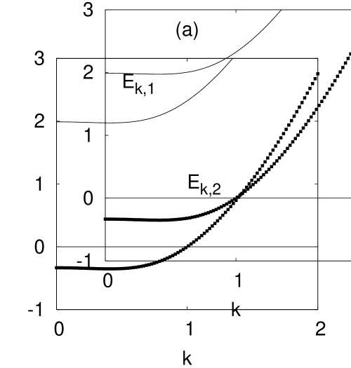
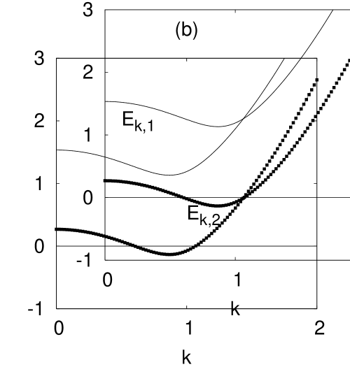
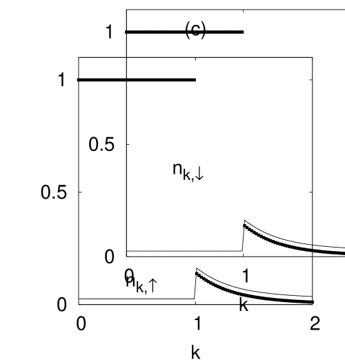
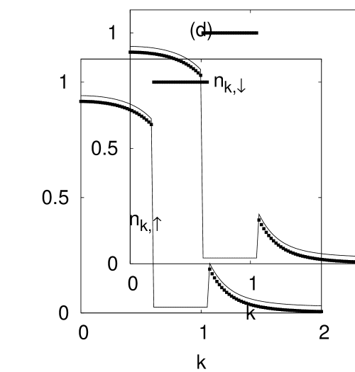
Figure 2: Schematic plots of $E_{\mathbf{k},1}$ (thin lines) and $E_{\mathbf{k},2}$ (thick lines) versus $k$ for (a) phase I and (b) phase II. Corresponding momentum distributions $n_{\mathbf{k},\uparrow}$ (thin lines) and $n_{\mathbf{k},\downarrow}$ (thick lines) are shown in (c) phase I and (d) phase II. Notice that the zero of $n_{\mathbf{k},\uparrow}$ is slightly shifted upwards from the zero of $n_{\mathbf{k},\downarrow}$, for better visualization.

The zero temperature momentum distributions

$$n_{\mathbf{k},\sigma}=\frac{1-\gamma_{\sigma}{\cal X}_{\mathbf{k},-}}{2}-\frac{\xi_{\mathbf{k},+}}{2E_{\mathbf{k},+}}{\cal X}_{\mathbf{k},+}$$ (19)

for phases I and II are extracted from Eq. (13). For momentum space regions where $E_{{\bf k},1}>0$ and $E_{{\bf k},2}>0$, the corresponding momentum distributions are equal $n_{{\bf k},\uparrow}=n_{{\bf k},\downarrow}$. However, when $E_{{\bf k},1}>0$ and $E_{{\bf k},2}<0$, then $n_{{\bf k},\uparrow}=0$ and $n_{{\bf k},\downarrow}=1$. We illustrate these cases in Figs. 2(c) and 2(d) for parameters of Figs. 2(a) and 2(b), respectively. Notice that the zero of $n_{\mathbf{k},\uparrow}$ is shifted slightly upwards to distinguish it from $n_{\mathbf{k},\downarrow}$ in the regions of momentum space where $n_{\mathbf{k},\uparrow}=n_{\mathbf{k},\downarrow}$. Although this topological transition is quantum ($T=0$) in nature, signatures of the transition should still be observed at finite temperatures within the quantum critical region, where the momentum distributions are smeared out due to thermal effects. Although the primary signature of this topological transition is seen in the momentum distribution, the isentropic $\kappa_{S}$ or isothermal $\kappa_{T}$ compressibilities and the speed of sound $c_{s}$ would have a cusp at the topological transition line similar to that encountered in $|\Delta_{0}|$ (see Fig. 1) as a function of the mass anisotropy $m_{r}$. The cusp (discontinuous change in slope) in $\kappa_{S}$, $\kappa_{T}$ or $c_{s}$ gets larger with increasing population imbalance.

Having discussed the finer topological classification of possible superfluid phases, we take all the criteria together (positive compressibility, positive curvature of thermodynamic potential, positive superfluid density, and topological character) to present next the resulting ground state phase diagrams.

III.3 Ground state phase diagrams

Based on all the previous criteria, we construct the $P$ versus $m_{r}$ phase diagram for seven sets of interaction strengths: $1/(k_{F,+}a_{F})=-2$, $-1$ and $-0.25$ on the BCS side shown in Fig. 3; $1/(k_{F,+}a_{F})=0$ at unitarity shown in Fig. 4; and $1/(k_{F,+}a_{F})=0.25$, $1$ and $2$ on the BEC side shown in Fig. 5. In these diagrams, the $\uparrow$ ($\downarrow$) label always corresponds to lighter (heavier) mass such that lighter (heavier) fermions are in excess when $P>0$ $(P<0)$. Notice that this choice spans all possible population imbalances and mass ratios.

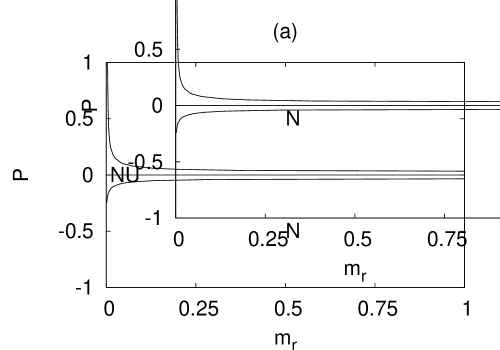
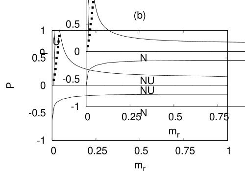
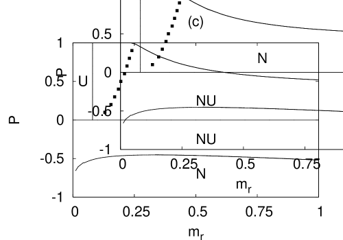
Figure 3: Phase diagram of $P=(N_{\uparrow}-N_{\downarrow})/(N_{\uparrow}+N_{\downarrow})$ versus $m_{r}=m_{\uparrow}/m_{\downarrow}$ on the BCS side when a) $1/(k_{F,+}a_{F})=-2$ b) $1/(k_{F,+}a_{F})=-1$ and c) $1/(k_{F,+}a_{F})=-0.25$. We show normal (N), uniform (U) or non-uniform (NU) superfluid phases. The dotted line (black squares) separate topologically distinct regions.

In Figs. 3-5, we indicate the regions of normal (N), and uniform (U) or non-uniform (NU) superfluid phases. The black squares indicate the transition line that separates topological phases I and II. In all phase diagrams, phase I (II) always appears to the left (right) of the dotted lines for $P>0$, while phase I (II) always appears to the right (left) of the dotted lines for $P<0$.

The normal phase is characterized by a vanishing order parameter ($\Delta_{0}=0$), while the uniform superfluid phase is characterized by $\rho_{0}(0)>0$ and $\partial^{2}\Omega_{0}/\partial\Delta_{0}^{2}>0$. The non-uniform superfluid phase is characterized by $\rho_{0}(0)<0$ and/or $\partial^{2}\Omega_{0}/\partial\Delta_{0}^{2}<0$, and it should be of the LOFF-type having one wavevector modulation only near the BCS limit FF ; LO , although closer to unitarity, we expect the non-uniform phase to be substantially different from the LOFF phases either having spatial modulation that would encompass several wavevectors or presenting complete phase separation between paired and unpaired fermions. However, from numerical calculations, the superfluid density criterion seems to be weaker for all parameter space and the non-uniform superfluid phase is characterized by $\partial^{2}\Omega_{0}/\partial\Delta_{0}^{2}<0$, which indicates possible phase separation, since at least one of the eigenvalues of the compressibility matrix $\kappa_{\sigma,\sigma^{\prime}}$ also becomes negative. Therefore, for a homogeneous system paired (or superfluid) fermions and unpaired (or excess) fermions coexist in the uniform superfluid regions, they are phase separated in non-uniform superfluid regions, and the topological transition from phase I to phase II may not be accessible. However, in a harmonic trap with a large superfluid region at the center, the topological phases should be observable since the central region is essentially a “uniform superfluid” with the excess fermions at the edge iskinmixture. The peculiar momentum distribution of different topological phases would be smeared out by the trapping potential, but their marked signatures should still be present. Furthermore, these topological phases may be accessible in trapped systems at finite temperature duan-qpt , or in optical lattices iskin-lattice .

As shown in Fig. 3(a) and 3(b), we find a small region of uniform superfluidity on the BCS side only when the mass anisotropy is small and the lighter fermions are in excess ($P>0$). Thus, to probe the largest amount of phases on the BCS side, mixtures consisting of ⁶Li and ⁴⁰K ($m_{r}\approx 0.15$) or ⁶Li and ⁸⁷Sr ($m_{r}\approx 0.07$) are good candidates. In the rest of the phase diagram, we find a quantum phase transition from the non-uniform superfluid to the normal phase beyond a critical population imbalance for both positive and negative $P$. The phase space of uniform superfluidity expands while that of the normal phase shrinks with increasing interaction strength as shown in Figs. 3(b) and 3(c).

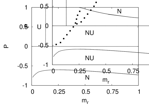
Figure 4: Phase diagram of $P=(N_{\uparrow}-N_{\downarrow})/(N_{\uparrow}+N_{\downarrow})$ versus $m_{r}=m_{\uparrow}/m_{\downarrow}$ at the unitarity limit when $1/(k_{F,+}a_{F})=0$. We show normal (N), uniform (U) or non-uniform (NU) superfluid phases. The dotted line (black squares) separate topologically distinct regions.

This general trend continues into the unitarity limit [$1/(k_{F,+}a_{F})=0$] as shown in Fig. 4. Since this limit is theoretically important as well as experimentally accessible, it is useful to analyze the phase diagram as a function of population imbalance and mass anisotropy. Notice that Fermi mixtures corresponding to mass ranges $0<m_{r}<0.23$, like ⁶Li and ⁸⁷Sr ($m_{r}\approx 0.07$) and ⁶Li and ⁴⁰K ($m_{r}\approx 0.15$) have phase diagrams which are qualitatively different from those corresponding to mass ratios $0.23<m_{r}<0.45$ like ⁶Li and ²⁵Mg ($m_{r}\approx 0.24$) and ⁶Li and ²H ($m_{r}\approx 0.33$), since a topological transition line may be accessible in the second range. Furthermore, only NU and N phases are accessible at unitarity for Fermi mixtures in the range of mass ratios $0.45<m_{r}<1$ like ⁴⁰K and ⁸⁷Sr ($m_{r}\approx 0.64$) or any equal mass mixtures. Notice that our results for the case of equal masses ($m_{r}=1$) are in close agreement with recent MIT experiments mit in a trap. At unitarity, our non-uniform superfluid to normal state boundary occurs at $P\approx\pm 0.73$, and the MIT group obtains $P\approx\pm 0.70(4)$ for their superfluid to normal boundary.

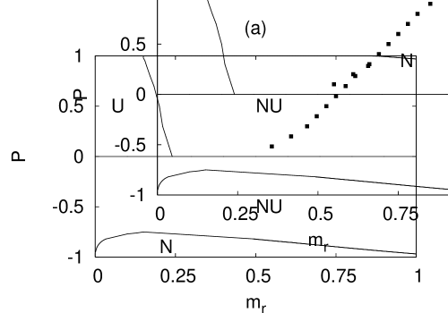
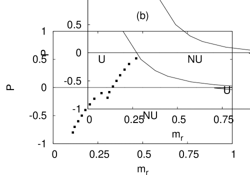
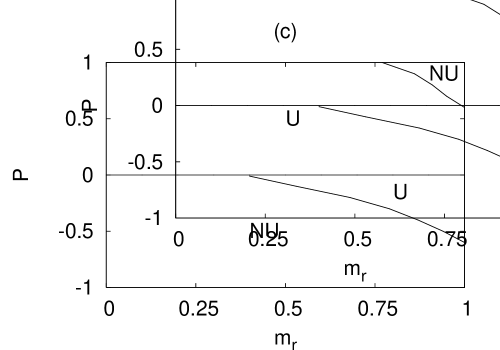
Figure 5: Phase diagram of $P=(N_{\uparrow}-N_{\downarrow})/(N_{\uparrow}+N_{\downarrow})$ versus $m_{r}=m_{\uparrow}/m_{\downarrow}$ on the BEC side when a) $1/(k_{F,+}a_{F})=0.25$, b) $1/(k_{F,+}a_{F})=1$ and c) $1/(k_{F,+}a_{F})=2$. We show normal (N), uniform (U) or non-uniform (NU) superfluid phases. The dotted line (black squares) separate topologically distinct regions.

Additional increase of interaction strength beyond unitarity on the BEC side leads to further expansion (shrinkage) of the uniform superfluid (normal) region as shown in Fig. 5(a) and 5(b). When heavier fermions are in excess ($P<0$), a uniform superfluid phase is not possible for any mass anisotropy until a critical interaction strength is reached. The critical interaction strength corresponds to $1/(k_{F,+}a_{F})\approx 0.8$ for $m_{r}=1$. Further increase of interaction strength towards the BEC limit [$1/(k_{F,+}a_{F})>1$], leads to further expansion (shrinkage) of the uniform (non-uniform) superfluid region as shown in Fig. 5(c), and only the uniform superfluid phase exists in the extreme BEC limit [$1/(k_{F,+}a_{F})\gg 1$] even for $P<0$ (not shown).

Having discussed the ground state phase diagrams, we present next fluctuation effects beyond the saddle point approximation.

IV Gaussian fluctuations

In this section, we discuss the (gaussian) fluctuation effects around the saddle point solutions at finite and zero temperatures. Near the critical temperature ($T\approx T_{c}$) we discuss the time-dependent Ginzburg-Landau (TDGL) equation, and at zero temperature ($T=0$) we analyse the collective phase (or Goldstone) mode as well as the effects of harmonic trap in the BEC limit, which are discussed next.

IV.1 Time-dependent Ginzburg-Landau equation near critical temperatures

Our basic motivation here is to investigate the low frequency and long wavelength behavior of the order parameter near $T_{c}$ where $\Delta_{0}=0$, and derive the TDGL equation carlos . We use the small $\mathbf{q}$ and $iv_{\ell}\to\omega+i\delta$ expansion of

$$L^{-1}(q)=\frac{1}{g}-\sum_{\mathbf{k}}\frac{1-n_{f}(\xi_{\mathbf{k}+\mathbf{q}/2,\uparrow})-n_{f}(\xi_{\mathbf{k}-\mathbf{q}/2,\downarrow})}{\xi_{\mathbf{k}+\mathbf{q}/2,\uparrow}+\xi_{\mathbf{k}-\mathbf{q}/2,\downarrow}-iv_{\ell}}|\Gamma_{\mathbf{k}}|^{2},$$

where $L^{-1}(q)=\mathbf{F}^{-1}_{1,1}(q)$, to obtain the TDGL equation

$$\left[a+b|\Lambda(x)|^{2}-\sum_{i,j}\frac{c_{ij}}{2}\nabla_{i}\nabla_{j}-id\frac{\partial}{\partial t}\right]\Lambda(x)=0$$ (20)

in the real space $x=(\mathbf{x},t)$ representation. Here, $n_{f}(x)=1/[\exp(\beta x)+1]$ is the Fermi distribution.

Expressions for the coefficients $a$, $b$, $c_{ij}$ and $d$ are presented in appendix B. The condition $a=0$ corresponds to the Thouless criterion, and the coefficient of the nonlinear term is positive ($b>0$) guaranteeing the stability of the effective theory. The kinetic energy coefficient $c_{ij}$ is an effective inverse mass tensor which reduces to a scalar $c$ in the s-wave case. The time-dependent coefficient $d$ is a complex number, and its imaginary part reflects the decay of Cooper pairs into the two-particle continuum for $\mu_{+}>0$. However, for $\mu_{+}<0$, the imaginary part of $d$ vanishes and the behavior of the order parameter $\Lambda(x)$ is propagating reflecting the presence of stable (long lived) bound states.

Since a uniform superfluid phase is more stable in the BEC side, we calculate analytically all coefficients in the BEC limit where $|\mu_{\pm}|\sim|\epsilon_{b}|/2\gg T_{\rm c}$. We obtain $a=a_{1}+a_{2}=-Vm_{+}^{2}(2\mu_{+}-\epsilon_{b})a_{F}/(8\pi)+Vm_{+}n_{e}a_{F}^{2}$, $b=b_{1}+b_{2}=Vm_{+}^{3}a_{F}^{3}/(16\pi)-Vm_{+}^{2}(\partial n_{e}/\partial\mu_{e})a_{F}^{4}$, $c=Vm_{+}^{2}a_{F}/[8\pi(m_{\uparrow}+m_{\downarrow})]$, and $d=Vm_{+}^{2}a_{F}/(8\pi)$. Here, $e$ labels the excess type of fermions and $n_{e}$ is the density of unpaired fermions. Through the rescaling $\Psi(x)=\sqrt{d}\Lambda(x)$, we obtain the equation of motion for a dilute mixture of weakly interacting bosons and fermions

$$-\mu_{B}\Psi(x) + \left[U_{BB}|\Psi(x)|^{2}+U_{BF}n_{e}(x)\right]\Psi(x)$$ (21)

$$- \frac{\nabla^{2}\Psi(x)}{2m_{B}}-i\frac{\partial\Psi(x)}{\partial t}=0,$$

with bosonic chemical potential $\mu_{B}=-a_{1}/d=2\mu_{+}-\epsilon_{b},$ mass $m_{B}=d/c=m_{\uparrow}+m_{\downarrow},$ and repulsive boson-boson $U_{BB}=Vb_{1}/d^{2}=4\pi a_{F}/m_{+}$ and boson-fermion $U_{BF}=Va_{1}/(dn_{e})=8\pi a_{F}/m_{+}$ interactions. This procedure also yields the spatial density of unpaired fermions given by

$$n_{e}(x) = [a_{2}/d+b_{2}|\Psi(x)|^{2}/d^{2}]/U_{BF}$$ (22)

$$= n_{e}-U_{BF}(\partial n_{e}/\partial\mu_{e})|\Psi(x)|^{2}.$$

Since $\partial n_{e}/\partial\mu_{e}>0$ the unpaired fermions avoid regions where the boson field $|\Psi(x)|$ is large. Thus, in a harmonic trap, the bosons condense at the center and the unpaired fermions tend to be at the edges. Notice that, Eq. (21) reduces to the Gross-Pitaevskii equation for equal masses with $P=0$ carlos , and to the equation of motion for equal masses with $P\neq 0$ pieri .

Next, we recall the standard definitions of the interactions in terms of the scattering lenghts $U_{BB}=4\pi a_{BB}/m_{B}$ and $U_{BF}=4\pi a_{BF}/m_{BF}$, where $m_{B}$ is the mass of the bosons and $m_{BF}=2m_{e}m_{B}/(m_{B}+m_{e})$ is twice the reduced mass of a boson of mass $m_{B}$ and an excess fermion of mass $m_{e}$. Combining these definitions with our results for $U_{BB}$ and $U_{BF}$ in terms of the fermion-fermion scattering length $a_{F}$, we can directly relate the boson-boson scattering parameter

$$a_{BB}=\frac{m_{B}}{m_{+}}a_{F}=\left[1+\frac{m_{\uparrow}}{2m_{\downarrow}}+\frac{m_{\downarrow}}{2m_{\uparrow}}\right]a_{F}$$ (23)

and the boson-fermion scattering parameter

$$a_{BF}=\frac{4m_{B}m_{e}}{m_{+}(m_{B}+m_{e})}a_{F}$$ (24)

to $a_{F}$. Notice that these expressions reduce to $a_{BB}=2a_{F}$ and $a_{BF}=8a_{F}/3$ for equal masses carlos ; pieri . A better estimate for $a_{BB}$ can be found in the literature gora .

Since the effective boson-fermion system is weakly interacting, the BEC temperature is $T_{c}=2\pi[n_{B}/\zeta(3/2)]^{2/3}/m_{B},$ where $\zeta(x)$ is the Zeta function and $n_{B}=(n-n_{e})/2$.

Notice that, the effective total number equation for the boson-fermion mixture can be written as

$$N\approx\sum_{\mathbf{k}}n_{f}(\xi_{\mathbf{k},e})+2\sum_{\mathbf{q}}n_{b}\left[\frac{|\mathbf{q}|^{2}}{2m_{B}}-\widetilde{\mu}_{B}\right],$$ (25)

where $n_{b}(\varepsilon)=1/[\exp(\beta\varepsilon)-1]$ is the Bose distribution and $\widetilde{\mu}_{B}\to 0^{-}$ includes also the Hartree shift. In the limit when $T_{c}\to 0$, we obtain the critical chemical potential for unpaired fermions at the normal-to-stable uniform superfluid boundary as given by $\mu_{e}=2^{2/3}(m_{+}/m_{e})\epsilon_{F,+},$ where $e=(\uparrow,\downarrow)$ labels excess type of atoms. Since, $\mu_{+}\to\epsilon_{b}/2$ in this limit, the critical chemical potential imbalance is given by $\mu_{-}=\gamma_{e}[-\epsilon_{b}/2+2^{2/3}(m_{+}/m_{e})\epsilon_{F,+}],$ where $\epsilon_{b}=-1/(m_{+}a_{F}^{2})$ is the binding energy, and $\gamma_{\uparrow}=+1$ and $\gamma_{\downarrow}=-1$.

This concludes our analysis for the homogenous mixture of two types of ultra-cold fermions at finite temperatures. Next we discuss collective excitations at zero temperature.

IV.2 Sound velocity at zero temperature

In order to obtain the collective mode spectrum, we use the effective action defined in Eq. (2) and express $\Lambda(q)=[\lambda(q)+i\theta(q)]/\sqrt{2}$ in terms of the amplitude $\lambda(q)$ and phase $\theta(q)$ fields, respectively. Using the matrix elements of $\mathbf{F}^{-1}$ defined in Eqs. (5) and (6) and described in appendix A, we can obtain the matrix elements of the fluctuation matrix in the rotated basis $(\lambda(q),\theta(q))$. The diagonal elements of the fluctuation matrix in the rotated basis become $\mathbf{M}^{-1}_{\lambda,\lambda}(q)=[\mathbf{F}^{-1}_{1,1}+\mathbf{F}^{-1}_{1,2}+\mathbf{F}^{-1}_{2,1}+\mathbf{F}^{-1}_{2,2}]/2$ and $\mathbf{M}^{-1}_{\theta,\theta}(q)=[\mathbf{F}^{-1}_{1,1}-\mathbf{F}^{-1}_{1,2}-\mathbf{F}^{-1}_{2,1}+\mathbf{F}^{-1}_{2,2}]/2,$ while the off-diagonal elements become $\mathbf{M}^{-1}_{\lambda,\theta}(q)=i[\mathbf{F}^{-1}_{1,1}-\mathbf{F}^{-1}_{1,2}+\mathbf{F}^{-1}_{2,1}-\mathbf{F}^{-1}_{2,2}]/2$ with $\mathbf{M}^{-1}_{\theta,\lambda}(q)=(\mathbf{M}^{-1}_{\lambda,\theta})^{*}(q).$

The collective modes are found from the poles of the fluctuation matrix $\mathbf{M}(q)$ determined by the condition $\det\mathbf{M}^{-1}(q)=0$, when the usual analytic continuation $iv_{\ell}\rightarrow w+i0^{+}$ is performed. The easiest way to get the phase collective modes is to integrate out the amplitude fields to obtain a phase-only effective action. To obtain the long wavelength dispersions for the collective modes at $T=0$, we consider $|P|\to 0$ or $k_{F,+}=k_{F,\uparrow}=k_{F,\downarrow}$ limit, and expand the matrix elements of $\mathbf{F}^{-1}(q)$ to second order in $|\mathbf{q}|$ and $w$ to get $\mathbf{M}_{\lambda,\lambda}^{-1}(q)=A+C|\mathbf{q}|^{2}-Dw^{2},$ $\mathbf{M}_{\theta,\theta}^{-1}(q)=Q|\mathbf{q}|^{2}-Rw^{2}$ and $\mathbf{M}_{\lambda,\theta}^{-1}(q)=iBw,$ such that

$$\mathbf{M}^{-1}(\mathbf{q},w)=\left(\begin{array}[]{cc}A+C|\mathbf{q}|^{2}-Dw^{2}&iBw\\ -iBw&Q|\mathbf{q}|^{2}-Rw^{2}\end{array}\right).$$

The expansion coefficients are given in the Appendix B. Thus, there are two branches for the collective excitations, but we focus only on the lowest energy one correponding to the Goldstone mode with dispersion $w(\mathbf{q})=v|\mathbf{q}|,$ where

$$v=\sqrt{\frac{AQ}{AR+B^{2}}}$$ (27)

is the speed of sound. Extra care is required when $P\neq 0$ since Landau damping causes collective excitations to decay into the two-quasiparticle continuum even for the s-wave case, since gapless fermionic (quasiparticle) excitations are present (see Fig. 2).

The BCS limit is characterized by the criteria $\mu_{+}>0$ and $\mu_{+}\approx\epsilon_{F,+}\gg|\Delta_{0}|$. The expansion of the matrix elements to order $|{\mathbf{q}}|^{2}$ and $w^{2}$ is performed under the condition $[w,|\mathbf{q}|^{2}/(2m_{+})]\ll|\Delta_{0}|$. The coefficient that couples phase and amplitude fields vanish ($B=0$) in this limit. Thus, there is no mixing between the phase and amplitude modes. The zeroth order coefficient is $A={\cal D},$ and the second order coefficients are $C=Q/3={\cal D}v_{F,\uparrow}v_{F,\downarrow}/(36|\Delta_{0}|^{2}),$ and $D=R/3={\cal D}/(12|\Delta_{0}|^{2}).$ Here, $v_{F,\sigma}=k_{F,\sigma}/m_{\sigma}$ is the Fermi velocity and ${\cal D}=m_{+}Vk_{F,+}/(2\pi^{2})$ is the density of states per spin at the Fermi energy. Thus, we obtain

$$v=\sqrt{\frac{v_{F,\uparrow}v_{F,\downarrow}}{3}}=\sqrt{v_{\uparrow}v_{\downarrow}},$$ (28)

with $v_{\sigma}=v_{F,\sigma}/\sqrt{3}$, which reduces to the Anderson-Bogoliubov relation when the masses are equal.

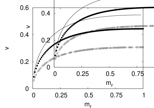
Figure 6: Sound velocity $v$ (in units of $v_{F,+}=k_{F,+}/m_{+}$) versus $m_{r}$ for $1/(k_{F,+}a_{F})=-1$ (solid line), $1/(k_{F,+}a_{F})=0$ (solid squares) and $1/(k_{F,+}a_{F})=1$ (hollow squares). Here, populations are equal ($P=0$).

On the other hand, the BEC limit is characterized by the criteria $\mu_{+}<0$ and $\xi_{\mathbf{k},+}\gg|\Delta_{0}|$. The expansion of the matrix elements to order $|{\mathbf{q}}|^{2}$ and $w^{2}$ is performed under the condition $[w,|\mathbf{q}|^{2}/(2m_{+})]\ll|\mu_{+}|$. The coefficient $B\neq 0$ indicates that the amplitude and phase fields are mixed. The zeroth order coefficient is $A=\kappa|\Delta_{0}|^{2}/(2|\mu_{+}|),$ the first order coefficient is $B=\kappa,$ and the second order coefficients are $C=Q=\kappa/[2(m_{\uparrow}+m_{\downarrow})]$ and $D=R=\kappa/(8|\mu_{+}|),$ where $\kappa={\cal D}/(32\sqrt{|\mu_{+}|\epsilon_{F,+}}).$ Thus, we obtain

$$v=\frac{|\Delta_{0}|}{\sqrt{4(m_{\uparrow}+m_{\downarrow})|\mu_{+}|}}=\sqrt{v_{\uparrow}v_{\downarrow}}$$ (29)

with $v_{\sigma}=\sqrt{2\pi n_{\sigma}a_{F}/m_{\sigma}^{2}}$. Notice that the sound velocity is very small and its smallness is controlled by the scattering length $a_{F}$. Furthermore, in the theory of weakly interacting dilute Bose gas, the sound velocity is given by $v_{B}=\sqrt{4\pi a_{BB}n_{B}/m_{B}^{2}}.$ Making the identification that the density of pairs is $n_{B}=n_{+}$, the mass of the bound pairs is $m_{B}=m_{\uparrow}+m_{\downarrow}$ and that the Bose scattering length is

$$a_{BB}=\frac{m_{B}}{m_{+}}a_{F}=\left[1+\frac{m_{\uparrow}}{2m_{\downarrow}}+\frac{m_{\downarrow}}{2m_{\uparrow}}\right]a_{F},$$ (30)

$v_{B}$ reduces to the well known Bogoliubov relation when the masses are equal. Therefore, the strongly interacting Fermi gas with two species can be described as a weakly interacting Bose gas at zero temperature as well as at finite temperatures iskin-mixture . Notice that $a_{BB}$ reduces to $a_{BB}=2a_{F}$ for equal masses jan in the Born approximation. A better estimate for $a_{BB}$ can be found in the literature gora .

In Fig. 6, we show the sound velocity as a function of the mass ratio $m_{r}$ for three values of the scattering parameter $1/(k_{F,+}a_{F})=-1,0$ and $1$ corresponding to the BCS side [$1/(k_{F,+}a_{F})=-1$], unitarity [$1/(k_{F,+}a_{F})=0$], and to the BEC side [$1/(k_{F,+}a_{F})=1$]. Notice that the speed of sound could be measured for a given $m_{r}$ using similar techniques as in the single species case $m_{r}=1$ thomas ; grimm .

This concludes our analysis for collective excitations in the homogenous mixture of a two types of fermions at zero temperature. We discuss next the effective field theory between paired and unpaired fermions.

IV.3 Weakly interacting paired and excess fermions (Bose-Fermi mixtures) at zero temperature

In this section, we concentrate on the BEC regime, where the paired and unpaired (excess) fermions can be described by a mixture of molecular bosons and fermions. In this limit, the resulting equation of motion is identical to Eq. (21) near the critical temperature, except that all parameters are evaluated at zero temperature. Thus, at low temperatures the system continues to behave as a dilute mixture of weakly interacting bosons (formed from paired fermions) and unpaired fermions, and can be described by the free energy density

$${\cal F}(\mathbf{x})=E(\mathbf{x})-\mu_{e}n_{e}(\mathbf{x})-\mu_{B}|\Psi(\mathbf{x})|^{2},$$ (31)

where the energy density is

$$E(\mathbf{x})=K_{B}+K_{F}+\frac{1}{2}U_{BB}|\Psi(\mathbf{x})|^{4}+U_{BF}n_{e}(\mathbf{x})|\Psi(\mathbf{x})|^{2}.$$

Here, $K_{B}$ is the kinetic energy density of bosons (assumed to be much smaller than all the other energies) and $K_{F}$ is the kinetic energy density of fermions. Averaging these energy densities over the spatial coordinates $F=\int d\mathbf{x}{\cal F}(\mathbf{x})/V$ leads to a ground state average free energy density

$$F=\frac{1}{2}U_{BB}n_{B}^{2}+U_{BF}n_{e}n_{B}+\frac{3}{5}\epsilon_{F,e}n_{e}-\mu_{e}n_{e}-\mu_{B}n_{B},$$

where $n_{e}$ ($n_{B}$) is the average density of fermions (bosons), and $\epsilon_{F,e}$ is the fermi energy of the excess fermions. Using the positivity of the Bose-Fermi compressibility matrix $\kappa_{\alpha,\beta}=\partial\mu_{\alpha}/\partial n_{\beta}$, where $\alpha,\beta=e,B$, one can show that bosons and fermions phase separate when the condition

$$n_{e}\geq\frac{4\pi}{3}\left(\frac{\pi}{m_{e}}\right)^{3}\left(\frac{U_{BB}}{U_{BF}^{2}}\right)^{3}$$ (32)

is satisfied viverit .

Using the boson-boson and boson-fermion interactions $U_{BB}=4\pi a_{BB}/m_{B}$ and $U_{BF}=4\pi a_{BF}/m_{BF}$, the scattering paramaters indicated in Eqs. (23) and (24), as well as the relations $|P|=n_{e}/n$, $n=n_{\uparrow}+n_{\downarrow}=k_{F,+}^{3}/(3\pi^{2})$ and $n_{B}=(n-n_{e})/2$, then phase separation occurs when

$$|P|\geq\frac{1}{2}\left(\frac{\pi}{8}\right)^{3}\left(\frac{m_{+}/m_{e}}{k_{F,+}a_{F}}\right)^{3}.$$ (33)

Here $e$ labels excess type of fermions, and $m_{e}$ is the mass of the unpaired fermions, and $m_{+}$ is twice the reduced mass of the $\uparrow$ and $\downarrow$ fermions. This expression is quantitatively correct in its region of validity, i.e., when $1/(k_{F,+}a_{F})\gg 1$, however, it still gives semi-quantitative results for $1/(k_{F,+}a_{F})\gtrsim 2$. For instance, in the case of an equal mass mixture, this expression would suggest that the resulting Bose-Fermi mixture is uniform when $1/(k_{F,+}a_{F})>2.5$ for $|P|\to 0.5$, and when $1/(k_{F,+}a_{F})>3.2$ for $|P|\to 1$. From our numerical calculations we find $1/(k_{F,+}a_{F})>1.9$ for $|P|\to 0.5$, and when $1/(k_{F,+}a_{F})>2.4$ for $|P|\to 1$.

The analytic expression given in Eq. (33) may be used as a guide for the boundary between phase separation (non-uniform) and the mixed phase (uniform) for any mixture of fermions. In particular, this relation serves as an estimator for the phase bounday for future experiments performed in the BEC limit of unequal mass fermions with population imbalance. This relation can be rewritten in terms of the mass ratio $m_{r}=m_{\uparrow}/m_{\downarrow}$ by realizing that the ratio $m_{+}/m_{e}=2m_{r}/(1+m_{r})$ when $\downarrow$ (heavier) fermions are in excess, and that $m_{+}/m_{e}=2/(1+m_{r})$ when $\uparrow$ (lighter) fermions are in excess. Thus, when $\downarrow$ (heavier) fermions are in excess, the critical polarization below which phase separation (non-uniform phase) occurs is

$$P_{c,\downarrow}^{(1)}=-\frac{1}{2}\left(\frac{\pi}{4k_{F,+}a_{F}}\right)^{3}\left(\frac{m_{r}}{1+m_{r}}\right)^{3},$$ (34)

while, when $\uparrow$ (lighter) fermions are in excess, the critical polarization above which phase separation (non-uniform phase) occurs is

$$P_{c,\uparrow}^{(1)}=+\frac{1}{2}\left(\frac{\pi}{4k_{F,+}a_{F}}\right)^{3}\left(\frac{1}{1+m_{r}}\right)^{3}.$$ (35)

Notice that in the equal mass ($m_{r}=1$) case $P_{c,\downarrow}^{(1)}=-P_{c,\uparrow}^{(1)}$ as required by symmetry.

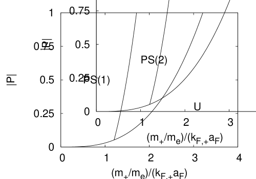
Figure 7: Phase diagram of $|P|=|N_{\uparrow}-N_{\downarrow}|/(N_{\uparrow}+N_{\downarrow})$ versus $(m_{+}/m_{e})/(k_{F,+}a_{F})$ in the BEC limit. We show the uniform superfluid (U) phase where paired and unpaired fermions coexist, and the phase separated non-uniform superfluid phases PS(1) and PS(2). The PS(1) region labels phase separation between pure unpaired (excess) and pure tightly paired fermions (bosons), while the PS(2) region labels phase separation between pure unpaired (excess) fermions and a mixture of unpaired and tightly paired fermions.

In addition, we can also describe analytically a finer structure of non-uniform (phase separated) superfluid phases deep into the BEC regime. For a weakly interacting Bose-Fermi mixture, the phase separated region consists two regions: PS(1), where there is phase separation between pure fermions and pure bosons (tightly paired fermions), and PS(2), where there is phase separation between pure fermions and a mixture of fermions and bosons (tighly bound fermions). Following the method of Ref. viverit , we obtain analytically the condition

$$n_{e}\geq\frac{1125\pi^{4}}{128m_{e}^{4}}\frac{U_{BB}^{3}}{U_{BF}^{6}}-\frac{5}{8}n_{B},$$ (36)

for the transition from the PS(2) to the PS(1) phase.

Using our effective boson-boson ($U_{BB}$) and effective boson-fermion $U_{BF}$ interactions, we can rewrite this relation as

$$|P|\geq\frac{8}{11}\left(\frac{15\pi}{64}\right)^{3}\left(\frac{m_{+}/m_{e}}{k_{F,+}a_{F}}\right)^{3}-\frac{5}{11},$$ (37)

where we used $n_{B}=(n-n_{e})/2$ as the boson density and $|P|=n_{e}/n$. These phase boundaries can also be expressed in terms of $m_{r}$ and $1/(k_{F,+}a_{F})$ as follows. When $\downarrow$ (heavier) fermions are in excess, the critical polarization below which the transition from PS(2) to PS(1) occurs is

$$P_{c,\downarrow}^{(2)}=-\frac{1}{11}\left(\frac{15\pi}{16k_{F,+}a_{F}}\right)^{3}\left(\frac{m_{r}}{1+m_{r}}\right)^{3}+\frac{5}{11},$$ (38)

while, when $\uparrow$ (lighter) fermions are in excess, the critical polarization above which the transition from PS(2) to PS(1) occurs is

$$P_{c,\uparrow}^{(2)}=+\frac{1}{11}\left(\frac{15\pi}{16k_{F,+}a_{F}}\right)^{3}\left(\frac{1}{1+m_{r}}\right)^{3}-\frac{5}{11}.$$ (39)

Notice that in the equal mass ($m_{r}=1$) case $P_{c,\downarrow}^{(2)}=-P_{c,\uparrow}^{(2)}$ as required by symmetry.

In Fig. 7, we show phase diagram of uniform and non-uniform superfluidity as a function of population imbalance $|P|$ and $(m_{+}/m_{e})/(k_{F,+}a_{F})$, which is strictly valid in the BEC limit when $1/(k_{F,+}a_{F})\gg 1$. In this figure, we show the uniform superfluid (U) phase where tightly paired and unpaired fermions coexist, and phase separated (non-uniform) superfluid (PS) phases. The PS(1) region labels phase separation between pure unpaired (excess) and pure tightly paired fermions (bosons), while the PS(2) region labels phase separation between pure unpaired (excess) fermions and a mixture of unpaired and tightly paired fermions. The phase boundary between U and PS(2) phases is determined from Eq. (33), and the phase boundary between PS(2) and PS(1) phases is determined from Eq. (37). For a fixed mass anisotropy $m_{r}$, when $|P|$ is large, we find phase transitions from PS(1) to PS(2) to U phase as the interaction strength $1/(k_{F,+}a_{F})$ increases. However, when $|P|$ is small, we find a phase transition from the PS(1) to the U phase as $1/(k_{F,+}a_{F})$ increases. This last result is unphysical and signals the breakdown of the approximations.

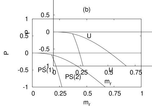
Figure 8: Phase diagram of $P=(N_{\uparrow}-N_{\downarrow})/(N_{\uparrow}+N_{\downarrow})$ versus $m_{r}=m_{\uparrow}/m_{\downarrow}$ in the BEC limit when (a) $1/(k_{F,+}a_{F})=3$ and (b) $1/(k_{F,+}a_{F})=4$. We show the uniform superfluid (U) phase where paired and unpaired fermion coexist, and phase separated non-uniform superfluid phases PS(1) and PS(2).

In Fig. 8, we show the phase diagram of population imbalance $P$ versus mass anisotropy $m_{r}=m_{\uparrow}/m_{\downarrow}$ in the BEC limit when (a) $1/(k_{F,+}a_{F})=3$ and (b) $1/(k_{F,+}a_{F})=4$. We indicate the uniform superfluid (U) phase where paired and unpaired fermion coexist, and phase separated non-uniform superfluid phases PS(1) and PS(2). The phase boundary between U and PS(2) phases is determined from Eq. (34) when $P<0$, and from Eq. (35) when $P>0$. In addition, the phase boundary between PS(2) and PS(1) phases is determined from Eq. (38) when $P<0$, and PS(1) phase does not exist when $P>0$. Notice that these phase diagrams are very similar to the one given in Fig. 5(c), with the added refinement of the non-uniform superfluid phases PS(1) and PS(2). For a fixed interaction strength $1/(k_{F,+}a_{F})$, when $|P|$ is large, we find phase transitions from PS(1) to PS(2) to U phase as the mass anisotropy $m_{r}$ increases. However, when $|P|$ is small, we find a phase transition from the PS(1) to the U phase as $m_{r}$ increases. This last result is unphysical and again signals the breakdown of the approximations.

To summarize, we analyzed analytically the structure of non-uniform (phase separated) superfluid phases in the BEC regime. However to understand the ultracold atomic experiments, one needs also to consider the trapping potential, which is discussed next.

IV.4 Effects of trapping potential

For simplicity, we approximate the trapping potential by an isotropic harmonic function where the potential energy is $V_{\sigma}(\mathbf{x})=\alpha_{\sigma}|\mathbf{x}|^{2}/2$ such that the local chemical potentials are given by

$$\mu_{\sigma}(\mathbf{x})=\mu_{\sigma}-\frac{1}{2}\alpha_{\sigma}|\mathbf{x}|^{2}.$$ (40)

Here, $\alpha_{\sigma}$ is proportional to the trapping frequency of the $\sigma$ type fermion, which is typically different for each kind of atom. In general, it is quite difficult to make completely isotropic traps and harmonic traps are typically elongated such that $V_{\sigma}(\mathbf{x})=\alpha_{\sigma,x}x^{2}/2+\alpha_{\sigma,y}y^{2}/2+\alpha_{\sigma,z}z^{2}/2$ with $\alpha_{\sigma,x}=\alpha_{\sigma,y}\gg\alpha_{\sigma,z}$. However, the same qualitative behavior occurs in the elongated or spherically symmetric (isotropic) traps, and we will confine ourselves for simplicity to the isotropic case. When experimental data becomes available and all the numbers are known, one can revisit this problem for detailed comparison between theory and experiment.

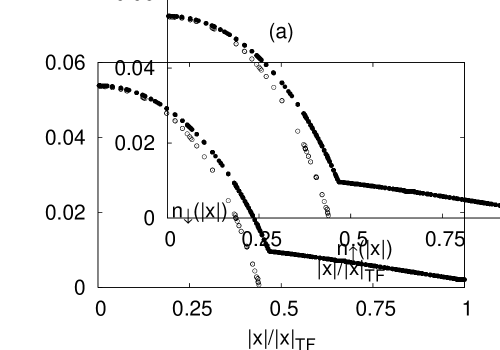
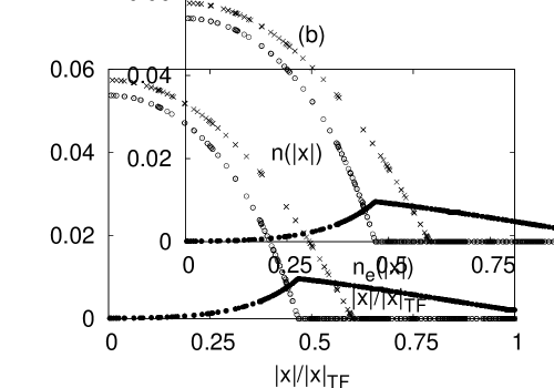
Figure 9: (a) Density $n_{\sigma}(|\mathbf{x}|)$ of fermions (in units of $k_{F,+}^{3}$), and (b) total density of fermions $n(|\mathbf{x}|)$ (hollow circles) and density of unpaired fermions $n_{e}(|\mathbf{x}|)$ (solid circles) versus trap radius $|\mathbf{x}|/|\mathbf{x}|_{TF}$. Here $P=0.5$ and $1/(k_{F,+}a_{F})=2$. In (b), we also compare $n(|\mathbf{x}|)$ for $P=0$ when $1/(k_{F,+}a_{F})=2$ (crosses).

Again, we confine our discussion to the BEC regime, and obtain the equation of motion for a dilute mixture of weakly interacting bosons and fermions at zero temperature

$$-\mu_{B}\Psi(x)+\left[U_{BB}|\Psi(x)|^{2}+U_{BF}n_{e}(x)\right]\Psi(x)+$$

$$[V_{\uparrow}(\mathbf{x})+V_{\downarrow}(\mathbf{x})]\Psi(x)-\frac{\nabla^{2}\Psi(x)}{2m_{B}}=i\frac{\partial\Psi(x)}{\partial t},$$ (41)

where the spatial density of unpaired fermions is

$$n_{e}(x)=n_{ex}(\mathbf{x})-U_{BF}\frac{\partial n_{ex}(\mathbf{x})}{\partial\mu_{e}}|\Psi(x)|^{2}.$$ (42)

These results are quite similar to the case of equal masses pieri . Notice that setting $V_{\sigma}=0$ reduces the problem to the free space case discussed in the previous subsection. Here, $n_{e}(\mathbf{x})=(1/V)\sum_{\mathbf{k}}n_{f}\left[\epsilon_{\mathbf{k},e}-\mu_{e}(\mathbf{x})\right],$ where $n_{f}(\varepsilon)=1/[\exp(\beta\varepsilon)+1]$ is the Fermi distribution. In the BEC limit when $a_{F}\to 0^{+}$, we can approximate the local density of unpaired fermions as

$$n_{e}(x)\approx\frac{1}{V}\sum_{\mathbf{k}}n_{f}\left[\epsilon_{\mathbf{k},e}-\mu_{e}(\mathbf{x})+U_{BF}|\Psi(x)|^{2}\right],$$ (43)

which at zero temperature leads to

$$n_{e}(\mathbf{x})=\frac{1}{6\pi^{2}}\{2m_{e}\left[\mu_{e}(\mathbf{x})-U_{BF}n_{B}(\mathbf{x})\right]\}^{3/2}.$$ (44)

Notice that the density of bosons at zero temperature is given by $n_{B}(\mathbf{x})=|\Psi(\mathbf{x})|^{2}$. Therefore, we need to solve Eq. (41) self-consistently with the number of unpaired (excess) $N_{e}=\int d\mathbf{x}n_{e}(\mathbf{x})$ and paired (bound) $N_{bf}=2\int d\mathbf{x}n_{B}(\mathbf{x})$ fermions such that the total number of fermions is $N=N_{e}+N_{bf}$.

Next we solve the self-consistency equations for a ⁶Li and ⁴⁰K mixture ($m_{r}=0.15$) within the Thomas-Fermi (TF) approximation, where the kinetic energy term in Eq. (41) is neglected. This leads to a coupled equation for density of paired and unpaired fermions

$$n_{B}(\mathbf{x})\approx\frac{\mu_{B}-V_{\uparrow}(\mathbf{x})-V_{\downarrow}(\mathbf{x})-U_{BF}n_{e}(\mathbf{x})}{U_{BB}}.$$ (45)

In our numerical analysis, we choose for convenience $\alpha_{\uparrow}=\alpha_{\downarrow}=\alpha$, $1/(k_{F,+}a_{F})=2$ and $P=0.5$ such that $N_{\uparrow}=3N_{\downarrow}$. However, in a more realistic case $\alpha_{\uparrow}\neq\alpha_{\downarrow}=\alpha$, since atoms with different masses may experience different trapping potentials due to their different polarizabilities.

In Fig. 9(a), we show the density $n_{\sigma}(|\mathbf{x}|)$ of $\sigma$ type fermion (in units of $k_{F,+}^{3}$) as a function of $|\mathbf{x}|/|\mathbf{x}|_{TF}$, where $|\mathbf{x}|_{TF}$ is the TF radius defined by $\epsilon_{F,+}=k_{F,+}^{2}/(2m_{+})=\alpha|\mathbf{x}|_{TF}^{2}/2$. We also scale the total number of fermions with $N=k_{F,+}^{3}|\mathbf{x}|_{TF}^{3}/24$. We find that the density of $\uparrow$ and $\downarrow$ fermions are similar close to the center of the trapping potential, while most of the excess fermions are close to the edges. In Fig. 9(b), we show the total density $n(|\mathbf{x}|)=n_{\uparrow}(|\mathbf{x}|)+n_{\downarrow}(|\mathbf{x}|)$ as well as unpaired fermions $n_{e}(|\mathbf{x}|)=n_{\uparrow}(|\mathbf{x}|)-n_{\downarrow}(|\mathbf{x}|)$. In both figures, we find a clear indication of phase separation between paired and unpaired fermions. In Fig. 9(b), we also compare the total density of fermions $n(|\mathbf{x}|)$ for the same parameters when the populations are balanced $N_{\uparrow}=N_{\downarrow}$. When $P\neq 0$, the total local density of fermions at the center of the trap is reduced in comparison to the $P=0$ case for the same fermion scattering parameter, since the unpaired fermions are pushed away from the center of the trap due to $U_{BF}$. These findings for unequal masses are similar to previous results on equal mass mixtures pieri ; torma ; yi ; chevy ; silva ; haque .

Lastly, for the parameters used, the harmonic trap tends to favor phase separation into a PS(1)-type phase where one has almost pure fermion and almost pure boson regions. In a harmonic trap it may be still possible to realize the PS(2)-type phase where one has an almost pure fermion region and an almost pure mixed phase of bosons and fermions, provided that good control over the trapping potentials is possible. Having concluded our discussion of the effects of a trapping potential, we present next the summary of our conclusions.

V Conclusions

In summary, we analyzed the phase diagram of ultra cold mixtures of two types of fermions (e.g., ⁶Li and ⁴⁰K; ⁶Li and ⁸⁷Sr; or ⁴⁰K and ⁸⁷Sr) from the BCS to the BEC limit as a function of scattering parameter, population imbalance, and mass anisotropy. We found that the zero temperature phase diagram of population imbalance versus scattering parameter is asymmetric for unequal masses, having a larger stability region for uniform superfluidity when the lighter fermions are in excess. This result is in sharp contrast with the symmetric phase diagram for equal masses.

In addition, we discussed topological quantum phase transitions associated with the disappearance or appearance of momentum space regions of zero quasiparticle energies when either the scattering parameter or population imbalance are changed. These quantum phase transitions are reflected in the momentum distribution as well as in thermodynamic properties, however they seem to lie in the non-uniform region of the phase diagram, but may survive at the center of a harmonic trap iskinprl . Furthermore this phase may be observable at finite temperatures in trapped systems duan-qpt , or in optical lattices iskin-lattice .

We also analyzed gaussian fluctuations around the saddle point order parameter both at finite and zero temperatures. Near the critical temperature, we derived the Ginzburg-Landau equation, and showed that it describes a dilute mixture of composite bosons (tightly bound fermions) and excess (unpaired) fermions in the BEC limit. At zero temperature, we obtained analytically the dispersion of collective excitations in the BCS and BEC limits, and showed numerically the evolution from the BCS to BEC regimes in the case of zero population imbalance. In addition, we discussed analytically how phase separation between paired fermions and excess fermions emerges analytically at zero temperature in the BEC limit. Lastly, we discussed the effects of a harmonic trapping potential, and concluded that phase separation between paired and unpaired fermions is favored even in the BEC limit.

VI Acknowledgements

We thank NSF (DMR-0304380) for support, and S.-K. Yip for e-mail correspondence regarding the stability criteria based on the compressibility matrix.

Appendix A Inverse fluctuation propagator

In this Appendix, we present explicitly the elements of the inverse fluctuation propagator $\mathbf{F}^{-1}(q)$. The diagonal matrix element of $\mathbf{F}^{-1}(q)$ is given by

$$\mathbf{F}_{1,1}^{-1}=\frac{1}{g} + \sum_{\mathbf{k}}\big{\{}v_{\frac{\mathbf{q}}{2}-\mathbf{k}}^{2}u_{\frac{\mathbf{q}}{2}+\mathbf{k}}^{2}\frac{n_{f}(E_{\frac{\mathbf{q}}{2}-\mathbf{k},1})-n_{f}(E_{\frac{\mathbf{q}}{2}+\mathbf{k},1})}{iv_{\ell}+E_{\frac{\mathbf{q}}{2}-\mathbf{k},1}-E_{\frac{\mathbf{q}}{2}+\mathbf{k},1}}$$ (46)

$$- u_{\frac{\mathbf{q}}{2}-\mathbf{k}}^{2}v_{\frac{\mathbf{q}}{2}+\mathbf{k}}^{2}\frac{n_{f}(E_{\frac{\mathbf{q}}{2}-\mathbf{k},2})-n_{f}(E_{\frac{\mathbf{q}}{2}+\mathbf{k},2})}{iv_{\ell}-E_{\frac{\mathbf{q}}{2}-\mathbf{k},2}+E_{\frac{\mathbf{q}}{2}+\mathbf{k},2}}$$

$$+ u_{\frac{\mathbf{q}}{2}+\mathbf{k}}^{2}u_{\frac{\mathbf{q}}{2}-\mathbf{k}}^{2}\frac{1-n_{f}(E_{\frac{\mathbf{q}}{2}+\mathbf{k},1})-n_{f}(E_{\frac{\mathbf{q}}{2}-\mathbf{k},2})}{iv_{\ell}-E_{\frac{\mathbf{q}}{2}+\mathbf{k},1}-E_{\frac{\mathbf{q}}{2}-\mathbf{k},2}}$$

$$- v_{\frac{\mathbf{q}}{2}+\mathbf{k}}^{2}v_{\frac{\mathbf{q}}{2}-\mathbf{k}}^{2}\frac{1-n_{f}(E_{\frac{\mathbf{q}}{2}-\mathbf{k},1})-n_{f}(E_{\frac{\mathbf{q}}{2}+\mathbf{k},2})}{iv_{\ell}+E_{\frac{\mathbf{q}}{2}-\mathbf{k},1}+E_{\frac{\mathbf{q}}{2}+\mathbf{k},2}}$$

$$\big{\}}|\Gamma_{\mathbf{k}}|^{2}$$

and the off-diagonal matrix element of $\mathbf{F}^{-1}(q)$ is given by

$$\mathbf{F}_{1,2}^{-1} = \sum_{\mathbf{k}}u_{\frac{\mathbf{q}}{2}+\mathbf{k}}v_{\frac{\mathbf{q}}{2}+\mathbf{k}}u_{\frac{\mathbf{q}}{2}-\mathbf{k}}v_{\frac{\mathbf{q}}{2}-\mathbf{k}}\big{\{}$$ (47)

$$\frac{n_{f}(E_{\frac{\mathbf{q}}{2}-\mathbf{k},1})-n_{f}(E_{\frac{\mathbf{q}}{2}+\mathbf{k},1})}{iv_{\ell}+E_{\frac{\mathbf{q}}{2}-\mathbf{k},1}-E_{\frac{\mathbf{q}}{2}+\mathbf{k},1}}$$

$$- \frac{n_{f}(E_{\frac{\mathbf{q}}{2}-\mathbf{k},2})-n_{f}(E_{\frac{\mathbf{q}}{2}+\mathbf{k},2})}{iv_{\ell}-E_{\frac{\mathbf{q}}{2}-\mathbf{k},2}+E_{\frac{\mathbf{q}}{2}+\mathbf{k},2}}$$

$$- \frac{1-n_{f}(E_{\frac{\mathbf{q}}{2}+\mathbf{k},1})-n_{f}(E_{\frac{\mathbf{q}}{2}-\mathbf{k},2})}{iv_{\ell}-E_{\frac{\mathbf{q}}{2}+\mathbf{k},1}-E_{\frac{\mathbf{q}}{2}-\mathbf{k},2}}$$

$$+ \frac{1-n_{f}(E_{\frac{\mathbf{q}}{2}-\mathbf{k},1})-n_{f}(E_{\frac{\mathbf{q}}{2}+\mathbf{k},2})}{iv_{\ell}+E_{\frac{\mathbf{q}}{2}-\mathbf{k},1}+E_{\frac{\mathbf{q}}{2}+\mathbf{k},2}}\big{\}}|\Gamma_{\mathbf{k}}|^{2}$$

where $u_{\mathbf{k}}^{2}=(1+\xi_{\mathbf{k},+}/E_{\mathbf{k},+})/2$ and $v_{\mathbf{k}}^{2}=(1-\xi_{\mathbf{k},+}/E_{\mathbf{k},+})/2,$ and $n_{f}(x)=1/[\exp(\beta x)+1]$ is the Fermi distribution.

For the s-wave case considered in this manuscript, a well defined low frequency and long wavelength expansion is possible in two limits: (I) at zero temperature ($T=0$) when population imbalance is zero $P=0$ such that the Fermi functions in Eqs. (46) and (47) vanish, and (II) near the critical temperature ($T\approx T_{c}$) where $|\Delta_{0}|\to 0$ such that $v_{\frac{\mathbf{q}}{2}\pm\mathbf{k}}$ (when $\xi_{\frac{\mathbf{q}}{2}\pm\mathbf{k},+}>0$) and $u_{\frac{\mathbf{q}}{2}\pm\mathbf{k}}$ (when $\xi_{\frac{\mathbf{q}}{2}\pm\mathbf{k},+}<0$) in Eqs. (46) and (47) vanish. Other than these two limits, there is Landau damping which causes the collective modes to decay into the two quasiparticle continuum.

Appendix B Expansion coefficients at $T=T_{c}$

In this Appendix, we derive the coefficients $a,b,c_{ij},d$ of the time dependent Ginzburg-Landau theory described in Eq. (20). We perform a small $\mathbf{q}$ and $iv_{\ell}\to w+i0^{+}$ expansion of the effective action near the critical temperature ($T\approx T_{c}$), where we assume that the fluctuation field $\Lambda(\mathbf{x},t)$ is a slowly varying function of $\mathbf{x}$ and $t$. The zeroth order coefficient $L^{-1}(0,0)$ is given by

$$a=\frac{1}{g}-\sum_{\mathbf{k}}\frac{X_{\mathbf{k},+}}{2\xi_{\mathbf{k},+}}|\Gamma_{\mathbf{k}}|^{2}$$ (48)

where $X_{\mathbf{k},\pm}=(X_{\mathbf{k},\uparrow}\pm X_{\mathbf{k},\downarrow})/2$ and $X_{\mathbf{k},\sigma}=\tanh(\beta\xi_{\mathbf{k},\sigma}/2).$ The second order coefficient $\partial^{2}L^{-1}(\mathbf{q},0)/(\partial q_{i}\partial q_{j})$ evaluated at $\mathbf{q}=0$ is given by

$$c_{i,j} = \sum_{\mathbf{k}}\left[\left(\frac{X_{\mathbf{k},\uparrow}Y_{\mathbf{k},\uparrow}}{m_{\uparrow}^{2}}+\frac{X_{\mathbf{k},\downarrow}Y_{\mathbf{k},\downarrow}}{m_{\downarrow}^{2}}\right)\frac{\beta^{2}k_{i}k_{j}}{32\xi_{\mathbf{k},+}}\right.$$ (49)

$$+ \left(\frac{2k_{i}k_{j}C_{-}}{m_{-}\xi_{\mathbf{k},+}}-\delta_{i,j}C_{+}\right)\frac{\beta}{16\xi_{\mathbf{k},+}}$$

$$+ \left.\left(\frac{\delta_{i,j}}{2m_{+}}-\frac{k_{i}k_{j}}{m_{-}^{2}\xi_{\mathbf{k},+}}\right)\frac{X_{\mathbf{k},+}}{4\xi_{\mathbf{k},+}^{2}}\right]|\Gamma_{\mathbf{k}}|^{2},$$

where $C_{\pm}=(Y_{\mathbf{k},\uparrow}/m_{\uparrow}\pm Y_{\mathbf{k},\downarrow}/m_{\downarrow})/2,$ and $Y_{\mathbf{k},\sigma}={\rm sech}^{2}(\beta\xi_{\mathbf{k},\sigma}/2).$ Here, $\delta_{i,j}$ is the Kronecker delta. The coefficient of the fourth order term is approximated by its value at $\mathbf{q}=\mathbf{0}$, and given by

$$b=\sum_{\mathbf{k}}\left(\frac{X_{\mathbf{k},+}}{4\xi_{\mathbf{k},+}^{3}}-\frac{\beta Y_{\mathbf{k},+}}{8\xi_{\mathbf{k},+}^{2}}\right)|\Gamma_{\mathbf{k}}|^{4},$$ (50)

The time-dependent coefficient has real and imaginary parts, and for the $s$-wave case is given by

$$d=\lim_{w\to 0}\sum_{\mathbf{k}}X_{\mathbf{k},+}\left[\frac{1}{8\xi_{\mathbf{k},+}^{2}}+i\pi\frac{\delta(2\xi_{\mathbf{k},+}-w)}{2w}\right]|\Gamma_{\mathbf{k}}|^{2}$$ (51)

where $\delta(x)$ is the Delta function.

Appendix C Expansion coefficients at $T=0$

In this Appendix, we perform a small $\mathbf{q}$ and $iv_{\ell}\to w+i0^{+}$ expansion of the effective action at zero temperature ($T=0$). From the rotated fluctuation matrix ${\mathbf{M}}^{-1}$ expressed in the amplitude-phase basis, we can obtain the expansion coefficients necessary to calculate the collective modes. We calculate the coefficients only for the case of zero population imbalance $P=0$, as extra care is needed when $P\neq 0$ due to Landau damping. In the long wavelength $(|\mathbf{q}|\to 0)$, and low frequency $(w\to 0)$ limits the condition $\{w,\frac{q_{i}q_{j}}{2m_{+}}\}\ll\min\{2E_{\mathbf{k},+}\},$ is used.

The coefficients necessary to obtain the matrix element $\mathbf{M}_{\lambda,\lambda}^{-1}(q)$ are

$$A=\sum_{\mathbf{k}}\frac{|\Delta_{0}|^{2}}{2E_{\mathbf{k},+}^{3}}$$ (52)

corresponding to the $(\mathbf{q}=0,w=0)$ term,

$$C = \sum_{\mathbf{k}}\left[\xi_{\mathbf{k},+}\frac{E_{\mathbf{k},+}^{2}-3|\Delta_{0}|^{2}}{8m_{+}E_{\mathbf{k},+}^{5}}-\left(\frac{E_{\mathbf{k},+}^{2}-10|\Delta_{0}|^{2}}{m_{+}^{2}}\right.\right.$$ (53)

$$+ \left.\left.\frac{10|\Delta_{0}|^{4}}{m_{+}^{2}E_{\mathbf{k},+}^{2}}+\frac{E_{\mathbf{k},+}^{2}-|\Delta_{0}|^{2}}{m_{-}^{2}}\right)\frac{k^{2}}{24E_{\mathbf{k},+}^{5}}\right]$$

corresponding to the $|\mathbf{q}|^{2}$ term, and

$$D=\sum_{\mathbf{k}}\frac{E_{\mathbf{k},+}^{2}-|\Delta_{0}|^{2}}{8E_{\mathbf{k},+}^{5}}$$ (54)

corresponding to the $w^{2}$ term.

The coefficients necessary to obtain the matrix element $\mathbf{M}_{\theta,\theta}^{-1}(q)$ are

$$Q=\sum_{\mathbf{k}}\left[\frac{\xi_{\mathbf{k},+}}{8m_{+}E_{\mathbf{k},+}^{3}}-\left(\frac{E_{\mathbf{k},+}^{2}-3|\Delta_{0}|^{2}}{m_{+}^{2}}+\frac{E_{\mathbf{k},+}^{2}}{m_{-}^{2}}\right)\frac{k^{2}}{24E_{\mathbf{k},+}^{5}}\right]$$ (55)

corresponding to the $|\mathbf{q}|^{2}$ term, and

$$R=\sum_{\mathbf{k}}\frac{1}{8E_{\mathbf{k},+}^{3}}$$ (56)

corresponding to the $w^{2}$ term.

The coefficient necessary to obtain the matrix element $\mathbf{M}_{\lambda,\theta}^{-1}(q)$ is

$$B=\sum_{\mathbf{k}}\frac{\xi_{\mathbf{k},+}}{4E_{\mathbf{k},+}^{3}}$$ (57)

corresponding to the $w$ term. These coefficients can be evaluated in the BCS and BEC limits, and are given in Sec. IV.2.

References

- (1) A. J. Leggett, in Modern Trends in the Theory of Condensed Matter (Springer-Verlag, Berlin 1980), p. 13.
- (2) P. Nozieres and S. Schmitt-Rink, J. Low. Temp. Phys. 59, 195 (1985).
- (3) C. A. R. Sá de Melo, M. Randeria, and J. R. Engelbrecht, Phys. Rev. Lett. 71, 3202 (1993).
- (4) M. W. Zwierlein, A. Schirotzek, C. H. Schunck and W. Ketterle, Science 311, 492 (2006).
- (5) G. B. Partridge, W. Lui, R. I. Kamar, Y. Liao, and R. G. Hulet, Science 311, 503 (2006).
- (6) W. V. Liu and F. Wilczek, Phys. Rev. Lett. 90, 047002 (2003).
- (7) S. -T. Wu and S. -K. Yip, Phys. Rev. A 67, 053603 (2003).
- (8) P. F. Bedaque, H. Caldas, and G. Rupak, Phys. Rev. Lett. 91, 247002 (2003).
- (9) J. Carlson and S. Reddy, Phys. Rev. Lett. 95, 060401 (2005).
- (10) C. H. Pao, S.-T. Wu, and S. K. Yip, Phys. Rev. B 73, 132506 (2006).
- (11) D. T. Son and M. A. Stephanov, Phys. Rev. A 74 013614 (2006).
- (12) D. E. Sheehy and L. Radzihovsky, Phys. Rev. Lett. 96, 060401 (2006).
- (13) T. L. Ho and H. Zhai, cond-mat/0602568.
- (14) A. Bulgac, M. M. Forbes and A. Schwenk, Phys.Rev.Lett. 97, 020402 (2006).
- (15) Z.-C. Gu, G. Warner, and F. Zhou, cond-mat/0603091.
- (16) T. Mizushima, K. Machida, and M. Ichioka, Phys. Rev. Lett. 94, 060404 (2005).
- (17) P. Pieri and G. C. Strinati, Phys. Rev. Lett 96, 150404 (2006).
- (18) J. Kinnunen, L. M. Jensen, and P. Torma , Phys. Rev. Lett. 96, 110403 (2006).
- (19) W. Yi and L. M. Duan, Phys. Rev. A 73, 031604 (2006).
- (20) F. Chevy, Phys. Rev. Lett. 96, 130401 (2006).
- (21) T. N. De Silva and E. J. Mueller, Phys. Rev. A 73, 051602(R) (2006).
- (22) M. Haque and H. T. C. Stoof, Phys. Rev. A 74, 011602 (2006).
- (23) L. Y. He, M. Jin and P. F. Zhuang, Phys. Rev. B 74, 024516 (2006).
- (24) M. Iskin and C. A. R. Sá de Melo, Phys. Rev. Lett. 97, 100404 (2006).
- (25) M. Iskin and C. A. R. Sá de Melo, cond-mat/0606624 (unpublished).
- (26) M. M. Parish, F. M. Marchetti, A. Lamacraft, B. D. Simons, cond-mat/0608651.
- (27) C. H. Pao, S.-T. Wu, and S. K. Yip, cond-mat/0604572.
- (28) E. Gubankova, A. Schmitt, and F. Wilczek, Phys.Rev. B 74 , 064505 (2006).
- (29) L. Y. He, M. Jin and P. F. Zhuang, cond-mat/0606322.
- (30) D. E. Sheehy and L. Radzihovsky, cond-mat/0608172.
- (31) C. H. Pao, S.-T. Wu, and S. K. Yip, cond-mat/0608501.
- (32) I. M. Lifshitz, Zh. Eksp. Teor. Fiz. 38, 1569 (1960).
- (33) G. E. Volovik, Exotic Properties of Superfluid , World Scientific, Singapore (1992).
- (34) L. S. Borkowski, and C. A. R. Sá de Melo, cond-mat/9810370 (unpublished).
- (35) R. D. Duncan and C. A. R. Sá de Melo, Phys. Rev. B 62, 9675 (2000).
- (36) S. S. Botelho, and C. A. R. Sá de Melo, Phys. Rev. B 71, 134507 (2005).
- (37) M. Iskin and C. A. R. Sá de Melo, Phys. Rev. Lett. 96, 040402 (2006).
- (38) P. Fulde and R. A. Ferrell, Phys. Rev. 135, A550 (1964).
- (39) A. I. Larkin and Y. N. Ovchinnikov, Sov. Phys. JETP 20, 762 (1965).
- (40) W. Yi and L. M. Duan, Phys. Rev. Lett. 97, 120401 (2006).
- (41) M. Iskin and C. A. R. Sá de Melo, cond-mat/0612496.
- (42) J. R. Engelbrecht, M. Randeria, and C. A. R. Sá de Melo, Phys. Rev. B 55, 15153 (1997).
- (43) D. S. Petrov, C. Salomon, and G. V. Shlyapnikov, J. Phys. B: At. Mol. Opt. Phys. 38, S645 (2005).
- (44) J. Kinast, A. Turlapov, and J. E. Thomas, Phys. Rev. Lett. 94, 170404 (2005).
- (45) M. Bartenstein, M. Bartenstein, A. Altmeyer, S. Riedl, S. Jochim, C. Chin, J. Hecker Denschlag, and R. Grimm, Phys. Rev. Lett. 92, 203201 (2004).
- (46) L. Viverit, C. J. Pethick, and H. Smith, Phys. Rev. A 61, 053605 (2000).