Complex systems Structures and organization in complex systems Networks and genealogical trees Order-disorder transformations; statistical mechanics of model systems

Scale-Freeness for Networks as a Degenerate Ground State: A Hamiltonian Formulation

Abstract

The origin of scale-free degree distributions in the context of networks is addressed through an analogous non-network model in which the node degree corresponds to the number of balls in a box and the rewiring of links to balls moving between the boxes. A statistical mechanical formulation is presented and the corresponding Hamiltonian is derived. The energy, the entropy, as well as the degree distribution and its fluctuations are investigated at various temperatures. The scale-free distribution is shown to correspond to the degenerate ground state, which has small fluctuations in the degree distribution and yet a large entropy. We suggest an implication of our results from the viewpoint of the stability in evolution of networks.

Complex networks have undergone a rapid surge of interest and a number of review articles already exist [1, 2]. A striking observation in this field is that many real networks have a broad scale-free like degree distribution. Why is this and what does it imply for the evolution mechanism of the networks? The preferential attachment [3] has been proposed as such a mechanism, where the scale-freeness is directly linked to the growing number of nodes in the network: once a link is in place it stays in place. This model mechanism has become a successful prototype explanation in many cases [1, 2]. In the present context, it corresponds to the extreme limit with only growing and no rewiring of links [4], whereas the opposite extreme is no growing and only rewiring. The fact that also the latter extreme can lead to scale-free degree distributions was explicitly demonstrated by the discovery of the merging-type evolution [5, 6], or the non-growth network model [7]. Furthermore, one can devise a scale-free evolution as an in-between of these two extremes. For example, you can combine slow growing with the merging type evolution and still get scale-free distributions [5] and you can combine preferential growing with deletion of nodes and also get broad degree distributions for somewhat less fast growing networks [8]. However, the distinction remains: In the one case the scale-freeness is linked to the network growing process and in the other to the rewiring of links.

In the present Letter, we try to get a better understanding of scale-freeness through rewiring by using a statistical mechanical formulation, applied for a non-network model without growing. We characterize this model in terms of a ground state energy, a temperature, and an entropy. It is found that the scale-free distribution is unique in the sense that it combines small deviations from the average degree distribution with a high entropy, or equivalently a large number of available states.

Our model consists of $N$ “towns” (=boxes) with the total of $N\langle k\rangle$ “inhabitants” (=balls) with $\langle k\rangle$ being the average number of inhabitants per town [9]. We assume that a randomly picked person $A$ chooses a person $B$ randomly and then moves to the $B$’s town with a certain probability. The rate of moving from a town with $k_{1}$ inhabitants to one with $k_{2}$ inhabitants, $R(k_{1},k_{2})$, is assumed to be separable, i.e., $R(k_{1},k_{2})=g(k_{1})f(k_{2})$, which means that the attraction or repulsion of a town of a certain size is the same for all people. The question is then what distribution of town sizes this leads to in a steady state. There is a one-to-one correspondence between this model and a corresponding network: The inhabitants corresponds to link-ends so that each link is associated with two specific persons. The link-ends are randomly chosen and randomly moved to other link-ends and attached to the same node. However, in networks one usually also introduces the topological constraints a) the network is connected, b) only one link connects two different nodes, and c) no link starts and ends on the same node. In practice these topological constraints only introduces significant statistical differences between the network and the town model for the case when the random rewiring in steady state leads to nodes with of order $N\langle k\rangle$ inhabitants[10].

The probability $P(k,t)$ that a town has $k$ inhabitants at time $t$ evolves following the master equation

$$N\frac{\partial P(k,t)}{\partial t}= -{\cal F}(k,t)f(k)+{\cal F}(k-1,t)f(k-1)$$ (1)

$$-{\cal F}(k,t)g(k)+{\cal F}(k+1,t)g(k+1),$$

where ${\cal F}(k,t)\equiv kP(k,t)/[\sum_{k}kP(k,t)]=kP(k,t)/\langle k\rangle$ is the probability of choosing a person from a town of size $k$. The two terms with the negative signs in Eq. (1) describe the decrease of $P(k)$ when a person moves in and out of a town of size $k$, respectively. Note that this for a network corresponds to rewiring one link at a time [11]. The two functions $f(k)$ and $g(k)$ are required to satisfy the condition $\sum_{k}kP(k)f(k)/\langle k\rangle=\sum_{k}kP(k)g(k)/\langle k\rangle=1$ in order to ensure that precisely one person on the average moves at each time step. The second and the last terms correspond to when a person moves from and to a town of size $k+1$ and $k-1$, respectively, which increase the inhabitants in the towns of size $k$. From the steady state condition together with the normalization conditions one obtains the detailed balance conditions for $f(k)$ for moving into a town, and $g(k)$ for moving out of a town. There is in fact only one possibility:

$$f(k) = \frac{(k+1)P(k+1)}{\left[1-\frac{P(1)}{\langle k\rangle}\right]kP(k)}\mbox{ \ \ for $k\geq 1$},$$ (2)

$$g(k) = \frac{1}{1-\frac{P(1)}{\langle k\rangle}}\mbox{ \ \ for}\ k\geq 2,$$ (3)

and $f(0)=0$ and $g(1)=0$. In this model, a sole inhabitant is not allowed to leave the town [$g(1)=0$], and you never move to an empty town because there is none to encounter [$f(0)=0$]. We stress that Eqs. (1)-(3) constitute the only possibility under the given assumptions.

The next step is to choose an update rule which is consistent with the above conditions: We start from two random persons $A$ and $B$. Suppose that $A$ ($B$) lives in a town of size $k_{1}$ ($k_{2}$). We then also randomly choose two persons $C$ and $D$ who live in towns of size $k_{2}+1$ and $k_{1}-1$, respectively. A possible update rule is that $A$ $either$ moves to $B$’s town $or$ $C$ moves to $D$’s town. We know from the detailed balance that the number of $A$’s moving to $B$’s is on the average equal to the number of $C$’s moving to $D$’s. The probability for $A$ to move to $B$’s town using this update is given by $\frac{f(k_{2})}{f(k_{2})+f(k_{1}-1)}$ and the probability for $C$ moving to $D$’s town is then $\frac{f(k_{1}-1)}{f(k_{2})+f(k_{1}-1)}$. The latter probability is then within this update rule equivalent to $A$ $not$ moving to $B$. Next, one notes that if we refer these two probabilities to moving or not moving $A$ to $B$’s town, respectively, then detailed balance is in fact automatically fulfilled. So our particular update rule is equivalent to randomly choosing two persons $A$ and $B$ and then moving $A$ to $B$’s town with the probability $\frac{f(k_{2})}{f(k_{2})+f(k_{1}-1)}$. The $relative$ probability for $A$ to move or not to move to $B$’s town, respectively, can consequently be expressed in terms of the Boltzmann-type factor $e^{\ln f(k_{2})-\ln f(k_{1}-1)}$. We rewrite this as $e^{-\Delta E}$ with $\Delta E_{1\rightarrow 2}=\ln f(k_{1}-1)-\ln f(k_{2})=\ln k_{1}P(k_{1})-\ln(k_{1}-1)P(k_{1}-1)-[\ln(k_{2}+1)P(k_{2}+1)-\ln k_{2}P(k_{2})]$ which is equivalent to assigning the energy $\epsilon(k)=\sum_{i=1}^{k}[\ln(iP(i))-\ln((i-1)P(i-1))]=\ln kP(k)$ to a town of size $k$. This means that the total energy of the Town model is

$$E=-N\sum_{k=1}P(k)\ln[kP(k)],$$ (4)

where $NP(k)$ is the average number of towns with $k$ inhabitants. We note that this implies that any predetermined distribution $P(k)$ can be recovered from a Monte Carlo (MC) algorithm with the canonical distribution $e^{-\hat{E}/T}$ with $T=1$ and $\hat{E}=-N\sum_{k=1}n(k)\ln[kP(k)]$, where $Nn(k)$ is the number of towns with $k$ inhabitants [12, 13]. The point in the present context is that $\hat{E}$ is the Hamiltonian for a given fixed $P(k)$ which yields the correct average energy $\langle\hat{E}\rangle=E=-N\sum_{k=1}P(k)\ln[kP(k)]$.

We also note that the relation between the entropy $S$ and the probability distribution $P(k)$ applies to the present case of a fixed number of people $N\langle k\rangle$ living in $N$ towns: There are then $N!$ ways to associate a given sequence of $N$ different labels with a town. However all towns with the same $k$ are equivalent. So the number of different states are $N_{s}=\frac{N!}{\Pi_{k}(NP(k))!}$  which by Stirling’s approximation gives the entropy

$$S=-N\sum_{k}P(k)\ln P(k).$$ (5)

This means that there is a one-to-one correspondence between $P(k)$ and $S$. Thus we can change variables and instead of keeping $P(k)$ fixed we keep $S$ fixed.

In order to find the extremum corresponding to these constraints we need three Lagrangian multipliers $a$, $b$, and $c$ corresponding to normalization condition for $P$, constant average number of people per town $\langle k\rangle$, and constant entropy $S.$ Thus in these variables the detailed balance condition determines $P(k)$ via the minimization of the functional [14]

$$G[P]=\sum_{k=1}P(k)[\ln kP(k)+a+bk-c\ln P(k)],$$ (6)

$\Longrightarrow\ln P(k)+\ln k+1+a+bk-c\ln P(k)-c=0$ and hence the solution

$$P(k)={\cal A}\frac{\exp(-k/\lambda)}{k^{\gamma}}$$ (7)

with $\gamma=1/(1-c)$, $\lambda=(1-c)/b$, and ${\cal A}=\exp(1-a/(1-c))$. We stress that Eq. (7) is unique and thus covers all possible solutions for the detailed balance equation of the form Eq. (1) except solutions with order $N\langle k\rangle$ inhabitants and other discrete solutions which fall outside variational calculus (see below). In order to finish the translation into a statistical mechanical formulation we observe that each of the possible solutions correspond to different free energies. In statistical mechanics such solutions correspond to different temperatures $T$. The solution for $T=0$ is the ground state and hence the absolute minimum of $G[P(k)={\cal A}\frac{\exp(-k/\lambda)}{k^{\gamma}}]$ with respect to the variables ${\cal A}$, $\lambda$, and $\gamma$. Minimization of $G[P]$ in Eq. (6) gives the ground state solution $P(k)={\cal A}k^{-\gamma_{0}}$ with ${\cal A}$ and $\gamma_{0}$ determined from the normalization and the constant $\langle k\rangle$ condition. Or, in other words $\gamma_{0}(\langle k\rangle)$ is a unique function of the average town population $\langle k\rangle$. Consequently, the Hamiltonian which gives the correct ground state is uniquely given by

$$H=N\sum_{k=1}n(k)\left(\frac{1}{\gamma_{0}}\ln n(k)+\ln k\right),$$ (8)

where $Nn(k)$ is the number of towns with $k$ inhabitants. (Note that the term $\sum_{k=1}n(k)[a+bk]$ has been dropped because it does not depend on $n(k)$). The statistical mechanics is specified by the Boltzmann factor given by $\exp(-H/T)$. The point is now that each one of the solutions $P(k)=A\frac{\exp(-k/\lambda)}{k^{\gamma}}$ are recovered as an statistical mechanical equilibrium solution; one for each temperature $T$. This completes the statistical mechanical formulation of the town model. This formulation is in accord with the entropy-maximum formulation by Jaynes [15] in the sense that the solution we obtain for each given $T$ contains the maximum unbiased information you can have subject to the imposed constraints.

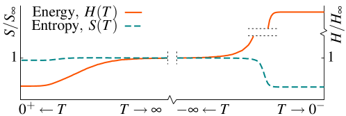
Figure 1: Energy $H(T)$ and entropy $S(T)$ as a function of $T$ for the town model. For $T=0$ the entropy is finite which means that the ground state is degenerate. As $T$ increases from $0$ to $\infty$, the entropy only increases slightly, which means that the ground state has almost as many available states as at $T=\infty$. On the negative-temperature side from $T=-\infty$ to $T=-0$ the energy increases whereas the entropy decreases since the number of available states decreases. (Note the cuts and shortenings of the horizontal and vertical axes.)

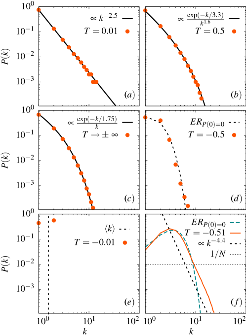
Figure 2: Distribution of town sizes $P(k)$ as a function of $T$ for $N=1000$ and $\gamma_{0}=2.5$ which gives $\langle k\rangle=1.56$. (a) For $T\simeq 0$ the distribution is scale-free. (b)-(c) As $T$ increases from $0$ to $\infty$, the scale-free distribution gradually changes to $P(k)\sim\exp(-k/\lambda)/k$. (d)-(e) As the temperature is increased through $-\infty$ to $-0$, the distribution continues to narrow and finally approaches as much as possible the single-sized town state in (d), where the vertical dashed line denotes the solution at $T=-0$ of the single-sized towns of the size $\langle k\rangle=1.56$. The solution for $T=-0.5$ is for practical purposes very close the the ER-solution denoted as a dashed curve in (d), for which the boundary condition $P(0)=0$ is used in the ER-calculation for the purpose of comparison. (f) Comparison for the case of $N=100$ and $\langle k\rangle=4$ between $P(k)$ at a negative $T$ and the ER distribution: As a larger value $\langle k\rangle=4$ is used, the difference is somewhat larger than in (d) for $\langle k\rangle=1.56$.

In Fig. 1, we plot the energy and entropy as functions of $T$: Both increase from $T=0$ to $T=\infty$, while from $T=-\infty$ to $T=-0$ the entropy decreases but the energy increases. The corresponding distribution of town sizes are illustrated in Fig. 2: It varies from the scale-free distribution with $\lambda=0$ at $T=0$ and then narrows to the totally random distribution with $\gamma=1$ and $\lambda>0$ at $T=\pm\infty$. On the negative-temperature side it continues to narrow down to $T=-0$. We stress that the Hamiltonian $H$ in Eq. (8) is the only Hamiltonian which contains the complete spectrum of possible solutions consistent with the detailed balance condition for the corresponding average distribution $P(k)$ Eq. (1). Also note that the Hamiltonian (8) includes the discrete solutions (which cannot be obtained directly from variational calculus).

From a dynamical point of view the town model evolves in time according to a Metropolis MC dynamics: At each time step a random person chooses another random person and moves or does not move to the town of the latter person according to a rate which depends on the energy difference given by the Hamiltonian. The point we are making is that this formulation combines maximum randomness with detailed balance [16, 17]: Provided that the only constraint is the detailed balance given by Eq. (1), then our description is unique and connects each solution $P(k)=\langle n(k)\rangle$ with the corresponding averaged fluctuations in time $\Delta(k)=\sqrt{\langle n(k)^{2}\rangle-\langle n(k)\rangle^{2}}$. Alternatively expressed: Our Metropolis algorithm defines the unique random rewiring process which gives rise to the average degree distribution $P(k)$ defined by Eq. (1).

Although Eq. (1) is a quite general form of detailed balance, it does not cover all possibilities. This is because there are alternative ways to introduce the randomness. A second possibility is to instead choose a random person and then a random town. This is described by the Hamiltonian $H=N\sum_{k}n(k)\ln k!$, and the corresponding distributions goes from single sized towns at $T=0$ to the ER(Erdős-Rényi) distribution at $T=\infty$ and continues towards the maximum entropy state $P(k)\sim\exp(-k/\lambda)$ on the negative-temperature side until it collapses to a discontinuous star-type distribution [18]: From a statistical mechanical point of a view the system collapses from a low-energy and high-entropy state via a first-order transition to a high-energy and low-entropy state [18]. The third obvious possibility is to choose two random towns, which only gives the trivial maximum entropy state $P(k)\sim\exp(-k/\lambda)$. We also note that our randomness ”random person to random person” is reminiscent of preferential attachment since choosing a random person is equivalent to choosing a random town with a probability $\sim kP(k)$ and then choosing one of its inhabitants with probability $1$. We note that distributions which are approximately of the ER-form are obtained for a negative $T$ in case of the random-person-to-random-person Hamiltonian as shown in Fig. 2. The deviation comes for the largest towns as is further illustrated in Fig. 2(f). The point here is that it is in practice difficult to distinguish between various random processes on the basis of only the distribution $P(k)$.

Our investigation of the town model suggests that the deviation, $\Delta(k)$, from the average distribution during a steady state process (or more generally any evolution process) is an essential and informative characteristics of a network which complements the average distribution function $P(k)$. In Fig. 3(a) the total noise $\Delta=\sum_{k}\Delta(k)$ is plotted as a function of $T$ for the town model. The most striking feature is the vanishing of $\Delta$ as $T\rightarrow+0$, which means that the deviation from the average $P(k)$ goes to zero. In the same limit $P(k)$ becomes scale-free and the number of available states is large, as discussed in connection with Figs. 1 and 2. As $T$ increases the noise also increases and goes through a maximum before it drops to zero when the number of available different states decreases to a number of order one. Figure 3(b) gives some examples of $\Delta(k)$ as a function of town size for some distributions: ”The smaller $T$ the smaller $\Delta(k)$”-connection is illustrated by the scale-free distribution for $T=0.05$ and $\langle k\rangle=2$ in Fig. 3(b). This is compared to the corresponding result for the preferential attachment, which gives the same $P(k)$ but a larger noise. In a similar way the large noise case for the ER-like distribution at $T=0.51$ and $\langle k\rangle=4$ is compared to the noise of the corresponding true ER-distribution (see Fig. 2(f)). As seen from Fig. 3(b) both have large deviations from the average distribution, although the ER-deviation is somewhat smaller.

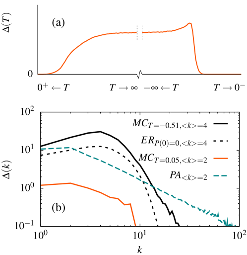
Figure 3: (a) Fluctuations $\Delta(T)$ as a function of $T$. As $T\longrightarrow+0$ the fluctuations vanish and the distribution $P(k)$ becomes scale-free. (b) The fluctuations $\Delta(k)$ as a function of the town size $k$ for a variety of distributions $P(k)$.

We have shown that the detailed balance under rather general conditions leads to a unique equilibrium Hamiltonian which connects the distribution function $P(k)$ to a fluctuation distribution $\Delta(k)$. In principle, this means that given a distribution $P(k)$ the corresponding fluctuation distribution will tell whether or not the dynamics of the system is consistent with detailed balance under the specified conditions. Thus the fluctuation distribution $\Delta(k)$ is a characteristics which complements the average distribution $P(k)$. Preliminary tests on some real networks suggest that this might be a useful characteristics in practice [18]. In addition, we have shown that the ground state of the Hamiltonian for the town model is the highly degenerate scale-free distribution. This state is characterized by many possible states combined with very small fluctuations. We speculate that, in as far as large changes and fluctuations might be fatal and many different possibilities beneficial for the evolution of a system, the scale-free distribution might sometimes be an evolutionary winner.

B.J.K. was supported by grant No. R01-2005-000-10199-0 from the Basic Research Program of the Korea Science and Engineering Foundation, P.M. and S.B. from Swedish VR contract 50412501.

References

- [1] Albert R. and Barabási A.-L., Rev. Mod. Phys., 74 (2002) 47.
- [2] Strogatz S., Nature, 410 (2001) 268; Dorogovtsev S. and Mendes J., Adv. Phys., 51 (2002) 1079; Evolution of Networks:From Biological Nets to the Internet and WWW (Oxford University Press, 2003); Newman M.E.J., Barabási A.-L. and Watts D.J., The Structure and Dynamics of Networks (Princeton University Press, 2006); Boccaletti S., Latora V., Morena Y., Chavez M. and Hwang D.-U., Phys. Rep., 424 (2006) 175.
- [3] Barabási A.-L., Albert R. and Jeong H., Science, 286 (1999) 509.
- [4] Both a growing network and preferential attachment of added links are required for the preferential attachment scheme to produce a scale-free distribution. See, e.g., [1].
- [5] Kim B.J., Trusina A., Minnhagen P. and Sneppen K., Eur. Phys. J. B, 43 (2005) 369.
- [6] Thurner S. and Tsallis C., Europhys. Lett., 72 (2005) 197.
- [7] Laird S. and Jensen H.J., Europhys. Lett., 76 (2006) 71.
- [8] Grönlund A., Sneppen K. and Minnhagen P., Physica Scripta, 71 (2005) 608.
- [9] Our model is a dynamic variant of the balls in boxes model. See, e.g., Bialas P., Bogacz L., Burda Z. and Johnston D., Nucl. Phys. B, 575 (2000) 599.
- [10] Minnhagen P. and Bernhardsson S., Chaos (in press).
- [11] Strictly speaking, it means that at each time step only a small fraction of the links can be simultaneously moved. This fraction has to be small enough for the chance of randomly picking two link-ends on the same node to be insignificant.
- [12] Burda Z., Correia J. and Krzywicki A., Phys. Rev. E, 64 (2001) 046118.
- [13] Berg J. and Lässig M., Phys. Rev. Lett., 89 (2002) 228701.
- [14] We are free to choose the sign of without affecting the content of the formulation.
- [15] Jaynes E.T., Phys. Rev., 106 (1957) 620.
- [16] Palla G., Derenyi I., Farkas I. and Vicsek T., Phys. Rev. E, 69 (2004) 046117.
- [17] Park J. and Newman M.E.J., Phys. Rev. E, 70 (2004) 066117.
- [18] Bernhardsson A. and Minnhagen P., Phys. Rev. E, 74 (2006) 026104.