Quantum Rings with Rashba spin orbit coupling: a path integral approach

Abstract

We employ a path integral real time approach to compute the DC conductance and spin polarization for electrons transported across a ballistic Quantum Ring with Rashba spin-orbit interaction. We use a piecewise semiclassical approximation for the particle orbital motion and solve the spin dynamics exactly, by accounting for both Zeeman coupling and spin-orbit interaction at the same time. Within our approach, we are able to study how the interplay between Berry phase, Ahronov Casher phase, Zeeman interaction and weak localization corrections influences the quantum interference in the conductance within a wide range of externally applied fields. Our results are helpful in interpreting recent measurements on interferometric rings.

I Introduction

In classical physics, a charged particle moving in an external magnetic field $B$ feels a (Lorentz) force only in the regions in which $B$ is different from zero. Instead, in 1959 Ahronov and Bohm (AB)aharonovbohm showed that the wave packet representing the state of a quantum particle can be influenced by an external vector potential $\vec{A}$, even if the corresponding magnetic field is zero, provided that the particle is moving in a space with a nontrivial topology (holes). To be more specific, the wavefunction of the charged particle may acquire a nonzero phase, when undergoing a closed path in a space threaded by an external magnetic flux.

Nowadays, mesoscopic quantum rings (QR’s) allow to have direct access to the phase of the electron wavefunction, since their size is smaller than the distance over which the phase randomizes, as a consequence of scattering against impurities and interactions. The total rate of particles coming from the two arms of the ring and interfering at the exit contact can be directly probed by measuring the QR conductance. Indeed, interference effects have been observed in metal QRs many years agowebb . In addition, since electrons are spinful particles, the spin part of the wavefunction is influenced by the magnetic field via the Zeeman term in the Hamiltonian. Moreover, a more subtle effect arises when there is a magnetic field non-orthogonal to the plane of the orbiting particle because, as a consequence of the orbital motion, its spin dynamics is instantaneously governed by a time-dependent Hamiltonian anandans . This time dependence ends up in an extra phase acquired by the particle wavefunction which is named after Berry berry ; anandan , who put in foreground its topological properties when the orbits are closed.

Recently, semiconductor technology allows to grow samples (for instance made by InAs or InGaAs) with sizeable spin orbit interaction (SOI). Rashbarashba first pointed out that the SOI strength can be controlled by means of voltage gates. This feature has been recently found experimentally meijer ; miller . Because of the SOI, an electric field $E$ orthogonal to the orbit provides a momentum dependent effective magnetic field felt by the electron spin in orbital motion. Such a field can be equally well described by a vector potential that adds an extra phase to the wavefunctionaronov . This phase was spelled out by Ahronov and Casher ac , as a “dual” AB effect, with charge and spin interchanged (together with $B$ and $E$).

During the last years, the effects of SOI on the AB oscillations have been observed in semiconductor based QR by several groups yau ; nitta ; morpurgo ; kato . It has been recognized that, in the presence of both $B$ and $E$ orthogonal to the orbit plane, the effective, momentum dependent total $B$ field is tilted w.r. to the vertical direction. The resulting Berry phase influences the interference pattern. Such a result is of the utmost interest because the Rashba-SOI (RSOI) turns out to be a tool to tune the Berry phase and, ultimately, the conductance, as well as the spin polarization of the outgoing electrons. In Ref. molenkamp , it is clearly shown that the AB interference fringes can be modified by tuning an external electrostatic potential.

In a recent publicationnoiletter we have included all these phenomena affecting the interference of an electron ballistically transported in a ring, also accounting for some dephasing at the contacts. We have also shown that the AB peak in the Fourier transform of the magnetoconductance displays satellite peaks due to the RSOI. It has been suggested that satellite peaks observed in recent experimentsshayegan have the same origin. In the present work we review the theory by presenting the full calculation. In addition, we include the semiclassical paths leading to weak localization correctionsnonloso , and we discuss the rotation of the spin polarization, during the transport across the ring.

During the last years, several theoretical techniques have been employed to study quantum transport in a QR. In Ref.s loss , an imaginary time path integral approachfeynman is developed to study the conductance of a strictly one dimensional (1D) QR and its conductance fluctuations in the diffusive limit. In Ref. tserkov a real time path integral approach is applied in the limit of negligible Zeeman splitting. Several papers have discussed the conductance properties and the spin selective transport of QR’s in the strictly 1D ballistic limit, by means of a spin dependent scattering matrix approach molnar ; frustaglia ; shen ; dario ; citro . In the absence of the magnetic flux, the conductance shows quasi-periodic oscillations in the SOI stength, which can be modified by switching the magnetic field on. Numerical calculations souma ; lozano ; wu have shown that in the 2D case there are only quantitative modifications of the 1D results that do not qualitatively affect the physics.

In this paper we extend the real time path integral approach previously developed in Ref.noiletter to study the conductance and the spin transport properties of a ballistic quantum ring in the presence of both RSOI and of an external magnetic flux orthogonal to the ring plane. We use a “piecewise” saddle point approximation for the orbital motion, keeping the full quantum dynamics of the spin. This approach allows us to take into account, in a nonperturbative way, both the RSOI and AB phase and to include also the Zeeman spin splitting.

Our numerical approach evaluates all paths contributing to the quantum propagator. The scattering at the leads can be forward or backward, according to the probability amplitudes given by the S-matrix. Weak localization corrections can be easily extracted from our result. We also allow for some diffusiveness at the contacts by adding a random phase factor in the motion.

The DC conductance is derived from the Landauer formula landauer ${\cal{G}}={e^{2}}/{\hbar}\sum_{\sigma\sigma^{\prime}}\left|A(\sigma;\sigma^{\prime}|E)\right|^{2}$, where $A(\sigma;\sigma^{\prime}|E)$ is the probability amplitude for an electron entering the ring with energy $E$ and spin polarization $\sigma^{\prime}$ to exit with spin polarization $\sigma$. We also report the change in the spin polarization the electron transported across the ring.

The structure of the paper is as follows:

• In Section II we introduce the Feynman propagator for a spinful electron injected at the Fermi energy in the ring.

• In Section III we discuss the topology of the allowed paths and the scattering of the electron at the leads.

• In Section IV we represent our path integral in the coherent spin basishaldane ; plet and derive the saddle point equations of motion, whose classical counterpart is described in detail in Appendix A. This allows us to justify the choice of a piecewise semiclassical approximation for the orbital motion of the electron in the ring.

• In Section V we present the details of the calculation by rewriting the path integral as a collection of single arm propagators. These are the building blocks to be calculated in the next section.

• In Section VI we analyze how the orbital motion affects the full quantum dynamics of the electron spin for each arm of the ring and chirality. The spin propagator is derived in Appendix B, in the basis corresponding to the rotating reference frame in the spin space.

• In Section VII we discuss the dependence of the conductance on the external fields and on the overall transmission across the ring.

• In Section VIII we focus on the spin polarization of the outcoming electron.

• Section IX includes a short summary and our conclusions.

II The transmission amplitude

Our model Hamiltonian will be the two-dimensional Hamiltonian for a particle with spin-1/2 $\vec{S}$, in an orthogonal magnetic field, with spin-orbit coupling to an orthogonal electric field (Rashba coupling). It is given by

$$H[\vec{p},\vec{r},\vec{S}]=\frac{1}{2m}\left(\vec{p}+\frac{e}{c}\vec{A}_{0}\right)^{2}-\omega_{c}\>S_{z}+{H}_{so}$$ (1)

$$H_{so}=\frac{2\alpha}{\hbar^{2}}\left({\hat{z}}{\times}\left({\vec{p}+\frac{e}{c}\vec{A}_{0}}\right)\right){\cdot}{\vec{S}}\>\>\>\>,$$

where $\alpha$ is the spin orbit coupling constant, in units $eV\>$Å, $\vec{S}=\hbar\vec{\sigma}/2$ (${\sigma_{x},\sigma_{y},\sigma_{z}}$ are the Pauli matrices), $\vec{A}_{0}(\vec{r})=\frac{B}{2}(-y,x,0)$ is the vector potential generating the uniform field $B$, normal to the ring surface, taken in the symmetric gauge, $\omega_{c}=geB/2mc$ is the cyclotron frequency. In real nanostructures based on InAs or InGaAs the $g$ factor can strongly deviate from the value of two. However the result we present here, are fully general as they depend on the ratio $\alpha/\hbar\omega_{c}R$ which can be tuned by acting on $\alpha$. Since we will assume only a single channel to be avaliable for electron propagation across the ring, we will picture the single channel ring as a $1-d$ circle of radius $R$, connected to two leads. Accordingly, the position of the particle within the ring is parametrized by the angle $\varphi$ and the vector potential has just the azimutal component $A_{\varphi}=\phi/2\pi R$, where $\phi$ is the magnetic flux threading the ring.

In order to study the conduction properties of the ring, one needs the propagation amplitude for an electron entering the ring with spin polarization $\mu_{0}$ to exit with spin polarization $\mu_{f}$, at energy $E_{0}$. This is given by

$$A(\mu_{f};\mu_{0}|E_{0})=\int_{0}^{\infty}\>\frac{dt_{f}}{\tau_{0}}\>e^{i\frac{E_{0}t_{f}}{\hbar}}\>\langle{\vec{r}}_{f},\mu_{f},t_{f}|{\vec{r}}_{0},\mu_{0},t_{0}\rangle\>\>\>\>,$$ (2)

where $\langle{\vec{r}}_{f},\mu_{f},t_{f}|{\vec{r}}_{0},\mu_{0},t_{0}\rangle$ is the amplitude for a particle entering the ring at the point $\vec{r}_{0}$ and at the time $t_{0}$ with spin polarization $\mu_{0}$ to exit at the point $\vec{r}_{f}$ at the time $t_{f}$ with spin polarization $\mu_{f}$. In our tensor product notation, we define $|{\vec{r}},\mu\rangle=|{\vec{r}}\rangle\>\otimes\>|\mu\rangle\$. $\tau_{0}=mR^{2}/(2\hbar)$ is the time scale for the quantum motion.

In order to compute $\langle{\vec{r}}_{f},\mu_{f},t_{f}|{\vec{r}}_{0},\mu_{0},t_{0}\rangle$ , we resort to a path integral representation for the orbital part of the amplitude. Since we parametrize the orbital motion of the particle in terms of the angle $\varphi$, we provide the pertinent Lagrangian, ${\mathcal{L}}_{orb}$, as a function of $\varphi,\dot{\varphi}$. It is given by

$${\mathcal{L}}_{orb}[\varphi(t),\dot{\varphi}(t),\vec{\sigma}]=\frac{m}{2}R^{2}\dot{\varphi}^{2}(t)-\frac{\phi}{\phi_{0}}\hbar\dot{\varphi}(t)+\frac{\alpha^{2}\>m}{2\hbar^{2}}+\frac{\hbar^{2}}{8mR^{2}}\>\>\>\>.$$ (3)

The last two contributions to Eq.(3) are a constant, coming from the spin-orbit term, and the Arthursmorette term, which is required when a path integration is performed in cylindrical coordinates. Since both contributions are constant, they can be lumped into the incoming energy $E_{0}$ and therefore they will be omitted henceforth. By taking into account the spin degree of freedom, as well, we represent the propagation amplitude as

$$\langle{\vec{r}}_{f},\mu_{f},t_{f}|{\vec{r}}_{0},\mu_{0},t_{0}\rangle=\langle{\vec{r}}_{f},\mu_{f}|e^{-i\int_{t_{0}}^{t_{f}}\>dt\>H}|{\vec{r}}_{0},\mu_{0},t_{0}\rangle=\int_{\varphi(t_{0})=\varphi_{0}}^{\varphi(t_{f})=\varphi_{f}}\!\!\!\!{\cal D}\varphi\>e^{-i\int_{0}^{t_{f}}dt\;\left[\tau_{0}\dot{\varphi}^{2}-q\dot{\varphi}\right]}\>\langle\mu_{f}|\hat{U}_{spin}(t_{f},t_{0})|\mu_{0}\rangle\>\>\>\>,$$ (4)

where $q=\phi/\phi_{o}$, $\phi_{o}$ being the flux quantum $hc/e$.

$$\hat{U}_{spin}(t_{f},t_{0})={\bf T}\exp\left[-\frac{i}{\hbar}\>\int_{t_{0}}^{t_{f}}dt^{\prime}\>\hat{H}_{spin}(t^{\prime})\right]\>\>\>.$$ (5)

is the full spin propagator and the spin Hamiltonian $\hat{H}_{spin}(t)$ is given by

$$\frac{1}{\hbar}\hat{H}_{spin}(t)=\left[\begin{array}[]{cc}\frac{\omega_{c}}{2}&\gamma\dot{\varphi}e^{-i\varphi(t)}\\ \gamma\dot{\varphi}e^{i\varphi(t)}&-\frac{\omega_{c}}{2}\end{array}\right]\>\>\>\>,$$ (6)

with $\gamma=2\alpha\tau_{0}/(\hbar R)$nota . In Sections IV and V we show that the amplitude of Eq.(4) can be approximated by choosing a piecewise semiclassical orbital motion for the particle in each arm of the ring, while keeping the full quantum dynamics of the spin. In particular, we will see that, within the physically relevant range of parameters, the orbital motion can be approximated as a uniform rotation (with constant angular velocity), which makes the spin dynamics to be the one of a spin-1/2 in an effective, rotating, external magnetic field. Yet, in order to explain how we deal with quantum backscattering at the contacts between ring and arms and corresponding dephasing effects, we will introduce our formalism in the next section, by discussing a simplified version of our problem: a spinless electron propagating across a mesoscopic ring.

III Feyman’s paths for a Spinless particle transmitted across a ring

In this section we introduce our formalism by computing the transmission amplitude for a spinless electron of mass $m$ and charge $-e$, traveling across the ring in an orthogonal magnetic field. For a realistic device, at each lead one has to take into account three possible scattering processes, consistently with the conservation of the total current. This is described in terms of a unitary $S-$matrix that, in the symmetric case in which the two arms are symmetric, is given by

$$\mathcal{S}=\left(\begin{array}[]{c c c}-\frac{1}{2}(1+\bar{r})&\frac{1}{2}(1-\bar{r})&\sqrt{\frac{1}{2}(1-\bar{r}^{2})}\\ \frac{1}{2}(1-\bar{r})&-\frac{1}{2}(1+\bar{r})&\sqrt{\frac{1}{2}(1-\bar{r}^{2})}\\ \sqrt{\frac{1}{2}(1-\bar{r}^{2})}&\sqrt{\frac{1}{2}(1-\bar{r}^{2})}&\bar{r}\end{array}\right)\>\>\>\>.$$ (7)

The numerical labeling of the S-matrix elements referring to the three terminals of each contact fork, are explained in Fig.(1, 1a). Assuming, for simplicity, that the scattering matrix is the same for both leads, Eq.(7) will hold both at the left-hand lead, and at the right-hand lead of the ring.

In particular, $\mathcal{S}_{3,3}=\bar{r}$ is the reflection amplitude for a wave coming from the left lead, $\mathcal{S}_{1(2),1(2)}=-\frac{1}{2}(1+\bar{r})$ the reflection amplitude for a wave incoming from the upper/lower arm, $\mathcal{S}_{1(2),2(1)}=\frac{1}{2}(1-\bar{r})$ is the transmission amplitude from the upper (lower) to the lower (upper) arm and $\mathcal{S}_{1(2),3}=\mathcal{S}_{3,1(2)}=\sqrt{\frac{1}{2}(1-\bar{r}^{2})}$ is the transmission amplitude from the upper/lower arm to outside of the ring.

In Fig.(1) we show the simplest paths of the electrons in the ring including forward scattering at the contacts, only. The contribution to the total amplitude coming from such paths, in which the electron enters the ring at an angle $\varphi_{0}$ at time $t_{0}$ and exits at $\varphi_{f}$ at time $t_{f}$, is given by

$${\cal{A}}(\varphi_{f},t_{f};\varphi_{0},t_{0})=\sum_{n=-\infty}^{+\infty}\int_{\varphi(t_{0})=\varphi_{i}}^{\varphi(t_{f})=\varphi_{f}+2\pi n}\!\!\!\!\!\!\!{\cal{D}}\varphi(\tau)\>e^{-i{\cal{S}}[\varphi[t)]/\hbar}$$

$$=\sum_{n=-\infty}^{+\infty}e^{-iq\>(\varphi_{f}-\varphi_{i}+2\pi n)}\int_{\varphi(t_{0})=\varphi_{i}}^{\varphi(t_{f})=\varphi_{f}+2\pi n}\!\!\!\!\!\!\!\!\!\!\!\!\!\!\!\!\!\!\!\!\!\!\!\!\!\!\!\!{\cal{D}}\varphi(t)\>e^{-i\frac{mR^{2}}{2\hbar}\int_{t_{0}}^{t_{f}}dt\>\dot{\varphi}^{2}(t)}\>,$$ (8)

where we have summed over paths in which the electron winds $n+1/2$ times in the ring, before exiting it. Positive (negative) $n$ values imply clockwise (counterclockwise) propagation along the ring.

This propagator can be evaluated exactly moran . However we report here just the saddle point evaluation, for comparison with the spinful case. Minimizing the action gives the classical equation of motion (together with the pertinent boundary conditions for a path winding $n+1/2$ times):

$$\ddot{\varphi}(t)=0\>\>\>;\varphi(t_{i})=\varphi_{i}\>,\varphi(t_{f})=\varphi_{f}+2\pi n\>\>\>\>.$$ (9)

Let us assume that the particle is injected in the ring at $\varphi_{0}=0$ and comes out at $\varphi_{f}=\pi$ in a time $T=t_{f}$. Eq.(8) gives:

$${\cal{A}}(\pi,0,t_{f})=e^{i\pi q}\>\sqrt{\frac{\tau_{0}}{\pi it_{f}}}\>{\sum_{n=-\infty}^{+\infty}}^{\prime}e^{-i\pi^{2}(2|n|-1)^{2}\tau_{0}/t_{f}-i2\pi nq}$$

$$\>\>\>\>,$$ (10)

where the prime in the sum takes into account the fact that one does not sum over $n=0$, and the square root at the prefactor accounts for the gaussian fluctuations. Of course, this propagator is periodic in $q$ of period $q=1$ up to a minus sign.

More involuted paths arise if one takes into account backscattering processes in which the electron can get backscattered within the same ring’s arm from which it is coming. For instance, the paths $(2f)$ and $(2h)$, as well as $(2g)$ and $(2i)$ in Fig.(2), include looping in opposite directions around the ring’s hole. Interference between clockwise and counterclockwise windings leads to weak localization corrections. We denote these corresponding paths (including also $(2c)$ and $(2d)$ ) as “reversed paths”$(RP)$. In our approach, all order paths are numerically generated up to the convergency and the $S-$matrix of Eq.(7 ) is implemented in the numerical algorithm.

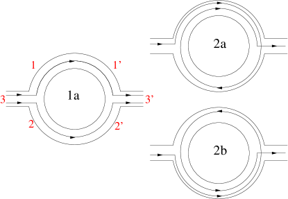
Figure 1: (color online) First and second order paths included in the calculation of the transmission amplitude across the ring, from left to right, including forward scattering only. Numbers $1,2,3(1^{\prime},2^{\prime},3^{\prime})$ in Fig. 1a refer to the labeling of the terminals in Eq.(7.)

Figure 2: Second order paths of the transmission amplitude from left to right including backscattering at the leads. Paths $(2f)$ and $(2h)$, as well as $(2g)$ and $(2i)$ contribute to the weak localization corrections.

In conclusion, we have established that the paths contributing to the transmission amplitude can be built up by adding four types of elementary paths: $u_{\rightarrow}$ forward orbiting in the upper arm of the ring ($\varphi\in(0,\pi)$), $u_{\leftarrow}$ backward orbiting in the upper arm of the ring ($\varphi\in(\pi,0)$), $d_{\rightarrow}$ forward orbiting in the lower arm of the ring ($\varphi\in(2\pi,\pi)$), $d_{\leftarrow}$ backward orbiting in the lower arm of the ring ($\varphi\in(\pi,2\pi)$). In Section V, we will generalize such an approach, while in the next Section we discuss the Feynman path-integral representation of the propagation amplitude for a spinful electron propagating along one of these elementary paths.

IV Quantum amplitude and semiclassical orbital motion for a spinful electron in the ring

In this section, we construct the Feynman representation in the basis of the coeherent spin states, for the propagation amplitude of an electron moving along one of the arms of the ring with a given chirality. To discuss the saddle-point approximation we need the equations of motion coming from the condition that the action is stationary. The coherent spin state basis provides a straightforward route to perform a semiclassical approximation involving both orbital, and spin degrees of freedom, at the same time. In particular, we will show under which conditions the classical orbital motion $\dot{\varphi}=cnst$, can be retained, as in the spinless case. Accordingly, the spin dynamics will be that of a “quantum magnetic moment” in a time-dependent external magnetic field.

Let $\Omega$ denote the orientation of the spin $\vec{S}$ and $|\Omega\rangle$ be the coherent state such that:

$$\langle\Omega|\hat{\vec{S}}|\Omega\rangle\equiv\vec{S}[\Omega]=\hbar\>S\>\left[\begin{array}[]{c}\sin\Theta\cos\Phi\\ \sin\Theta\sin\Phi\\ \cos\Theta\end{array}\right]\>\>\>\>,$$ (11)

for the three components of the spin vector, respectively. The full propagator in the coherent spin state representation is given by:

$$\langle\varphi_{f},\Omega_{f},t_{f}\>|\varphi_{0},\Omega_{0},0\rangle=\int_{\varphi(0)=\varphi_{0}}^{\varphi(t_{f})=\varphi_{f}}\!\!\!\!{\cal D}\varphi\>e^{-i\int_{0}^{t_{f}}dt\;\left[\tau_{0}\dot{\varphi}^{2}-q\dot{\varphi}\right]}\int_{\Theta(0)=\Theta_{0}}^{\Theta(t_{f})=\Theta_{f}}\!\!\!\!{\cal D}\Theta\int_{\Phi(0)=\Phi_{0}}^{\Phi(t_{f})=\Phi_{f}}\!\!\!\!{\cal D}\Phi\>\>e^{-\frac{i}{\hbar}{\cal{S}}_{spin}\left[\Theta,\dot{\Theta};\Phi,\dot{\Phi}|\varphi,\dot{\varphi}\right]}\>\>\>\>,$$ (12)

where:

$${\cal{S}}_{spin}\left[\Theta,\dot{\Theta};\Phi,\dot{\Phi}|\varphi,\dot{\varphi}\right]/\hbar=\int_{0}^{t_{f}}dt\;\left\{\frac{(1-\cos\Theta)}{2}\dot{\Phi}+{\cal{L}}_{spin}\left[\Theta,\dot{\Theta};\Phi,\dot{\Phi}|\varphi,\dot{\varphi}\right]\right\}\>\>\>\>.$$ (13)

with:

$${\cal L}_{spin}\left[\Theta,\dot{\Theta};\Phi,\dot{\Phi}|\varphi,\dot{\varphi}\right]=\frac{\omega_{c}}{2}\cos\Theta-\gamma\dot{\varphi}\sin\Theta\cos(\varphi-\Phi)\>\>\>\>.$$ (14)

The Lagrangian of Eq.(14) corresponds to the coherent spin-state representation of the classical Lagrangian derived from Eq.(1)

$${\cal L}[\varphi,\dot{\varphi},\vec{S}]=$$

$$\frac{m}{2}\dot{\vec{r}}^{2}-\frac{e}{c}\>\dot{\vec{r}}\cdot\vec{A}+2m\alpha\left[\hat{z}\cdot\left(\dot{\vec{r}}\times\vec{S}\right)\right]+\frac{m\alpha^{2}}{\hbar^{2}}+\omega_{c}S_{z}\>.$$ (15)

In Eq.(15) we have introduced the constraint that the orbital electron motion takes place along a one-dimensional circle by parametrizing the trajectories with the angle $\varphi$ as $x=R\cos\varphi;\;y=R\sin\varphi$. The additional Berry phase term aurbach in Eq.(13) arises from the fact that different spin coherent states are not orthogonal to each other since, to leading order in $\epsilon$, the scalar product between spin-coherent states at times $t_{j},t_{j}+\epsilon$, $|\Omega(t_{j})\rangle$ and $|\Omega(t_{j}+\epsilon)\rangle$ is given by

$$\langle\Omega(t_{j}+\epsilon)|\Omega(t_{j})\rangle\approx\exp\left[\frac{i}{2}[1-\cos\Theta(t_{j})]\dot{\Phi}(t_{j})\epsilon\right]\>\>\>\>.$$ (16)

Let us look for the trajectories in orbital and spin space which make the action stationary. This requires solving the Eulero-Lagrange equations for the Lagrangian ${\cal L}[\varphi,\dot{\varphi};\Theta,\dot{\Theta};\Phi,\dot{\Phi}]$ appearing in Eq.(12), which are given by

$$\frac{\dot{\Theta}}{2}\sin\Theta+\gamma\dot{\varphi}\>\sin\chi\>\sin\Theta = 0\>,$$ (17)

$$\sin\Theta[-\dot{\Phi}+\omega_{c}]+2\gamma\dot{\varphi}\>\cos\Theta\>\cos\chi = 0\>,$$ (18)

$$\ddot{\varphi}-\frac{\gamma}{2\tau_{0}}[\dot{\Theta}\>\cos\Theta\>\cos\chi+\dot{\Phi}\>\sin\Theta\>\sin\chi] = 0\>,$$ (19)

with $\chi=\varphi-\Phi$.

In order to extract the relevant physics from the above equations, we multiply Eq.(19) by $\dot{\varphi}$, and, by use of Eqs.(17,18), we rewrite Eq.(19) as:

$$\dot{\varphi}\ddot{\varphi}=-\frac{\omega_{c}}{4\tau_{0}}\>\dot{\Theta}\>\sin\Theta\>\>\>\>.$$ (20)

A straightforward time integration gives:

$$\tau_{0}\frac{(\dot{\varphi})^{2}}{2}-\frac{\omega_{c}}{4}\cos\Theta=cnst\>\>\>\>,$$ (21)

which states that the total energy is conserved. According to Eq.(21), the particle energy only includes the orbital kinetic term and the Zeeman term. This is obvious, since the force associated to the spin orbit coupling, being gyroscopic, does no work. A change in the precession angle $\Theta$ implies acceleration in the orbital motion. According to the spin Hamiltonian of Eq.(6) the RSOI is responsible for flipping of the spin, while the Zeeman coupling tends to stabilize the spin direction. Hence, there are two physically relevant limits, in which the orbital motion fully decouples from the spin dynamics, according to the inequality $\omega_{c}/2<(>)\dot{\varphi}$, as we are going to show next. Both limits involve an orbital motion with constant velocity $\dot{\varphi}$ and a spin orientation given by the angles $\Theta={\rm constant}\>\>\>,\>\>\varphi-\Phi=0\>(mod.\>\pi)$.

a) Vanishing Zeeman coupling: This case has already been considered and it has been shown that it can be exactly solved analyticallytserkov . In this case Eq.(20) allows for the semiclassical solution $\dot{\varphi}=cnst$ and quantum fluctuations of the spin do not interfere with the orbital motion. The spin is tilted by the constant angle $\tan\Theta=2\gamma$ and precesses with a constant frequency $\dot{\Phi}=\dot{\varphi}$.

b) Large Zeeman coupling: flipping of the spin and quantum fluctuations of the spin are strongly disfavoured, again corresponding to the classical saddle point configuration $\Theta={\rm constant}\>\>\>,\>\>\varphi-\Phi=0,\pi$ with

$$\pi/t_{f}=\dot{\varphi}=\pm\dot{\Phi}=\omega_{c}\>\frac{1}{1-2\gamma\>{\rm ctan}\Theta}\>\>\>.$$ (22)

The spin precesses around the $z$-axis, with the same angular velocity as the orbital motion. When $\gamma\to 0$, $\Theta$ can be vanishingly small, with $\dot{\Phi}=\omega_{c}$.

It may appear that the simple spin precession provided by Eq.(20) with $\Theta=cnst$ is a solution of Eq.s(17,18,19) for any ratio $\omega_{c}/\dot{\varphi}$. Were this the case, there would be no need to invoke the limitations of case $b)$ as stated above. However, a careful analysis of the stability of this saddle point solution shows that the simple spin precession is a minimum of the action only when the Zeeman coupling is strong. In particular, if $\omega_{c}/\dot{\varphi}>>1$, an additional condition $\omega_{c}\tau_{o}/\gamma^{2}>1$ has to be satisfied. Otherwise the frequency of the fluctuations around the saddle point solution does not keep real and the analysis of small oscillations in the parameter space around the saddle point solution breaks down.

This shows that a classical orbital motion with constant velocity is compatible with both limits of large and small ratios of the Zeeman coupling to the RSOI strength. However the two limiting cases do not belong to the same saddle point. In particular there will be a crossover region connecting the two limits in which quantum fluctuations of the spin may induce changes in the orbital velocity of the particle.

In the rest of the paper we will choose $\dot{\varphi}=const$ piecewise and parametrize the quantum dynamics of the spin with the value of the velocity obtained by the stationary phase condition discussed in the next section. As discussed above, our approximation cannot reproduce faithfully the intermediate region of parameters ranging the two limits of large and small Zeeman coupling $\omega_{c}/\gamma\dot{\varphi}<(>)1$. We checked numerically the reliability of our approximation, by numerically integrating Eqs.(17,18,19) and have have found that it is satisfactory in most of the parameter range.

By putting $\dot{\varphi}=cnst$ into Eqs.(17,18), they become, as we show in detail in Appendix A, the classical equations of motion for a magnetic moment in a time dependent magnetic field ${\cal{B}}\equiv({\cal{B}}_{+},{\cal{B}}_{-},{\cal{B}}_{z})=\left(\gamma\dot{\varphi}\>e^{i\varphi},\gamma\dot{\varphi}\>e^{-i\varphi},-\omega_{c}/2\right)$. This can be easily understood from the fact that minimizing the action in Eq.(12) directly w.r. to the spin components provides:

$$\vec{S}\times\frac{d\vec{S}}{dt}=-\frac{\delta H}{\delta\vec{S}}\>\>\>\>,$$ (23)

which has to be solved together with the constraint of constant modulus: $\vec{S}\cdot d\vec{S}/dt=0$ ( see Eq.(60).

Among the other possible saddle-points, a solution of the motion equations can be found with the particle trapped within the ring arm (turning points of $\varphi(t)$ are at $\varphi=0,\pi$) if $\gamma$ is large enough. This solution doesn’t seem to be practical as it requires fine tuning of the external parameters with transfer of energy from the spin motion to the orbital motion and viceversa. We have not investigated it in detail, but we expect that it could provide resonant tunneling across the ring.

V Saddle point approximation and looping in the ring

In this Section we show how we implement the piecewise saddle point solution for the orbital motion, $\dot{\varphi}=cnst$, to study the coherent propagation of the electron inside the ring. In the following, we will denote by “loop” and “looping trajectory“ both trajectories that wind around the ring (closed), and paths in which the particle moves forth and back in one of the ring arms (open) (see Fig.(2)). Of course, the amplitudes differs very much in these two types of looping . Indeed, the net spin rotation is different between the two paths and, also, the Ahronov-Bohm ($AB$) phase is absent in the latter ones .

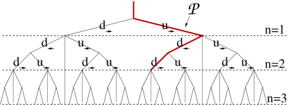
Figure 3: (color online) Cayley tree describing the way in which higher order paths are built in the numerical code. Full lines correspond to propagation in the upper arm ( $u$ ) or lower arm ( $d$) in the forward ($\rightarrow$) or backward ( $\leftarrow$) direction. The nodes represent the leads of the ring. The exit nodes are marked by a broken line at each order $n$. The heavy line correspond to the path reported in Eq.(25).

In general, at order $n$, we will have $2^{(2|n|-1)}$ trajectories of a particle entering the ring at $\varphi=0$ and exiting at $\varphi=\pi$ and each of them will include $2|n|-1(n=\pm 1,\pm 2,...)$ elementary paths (or “stretches”) of the type $u_{\rightarrow},u_{\leftarrow},d_{\rightarrow},d_{\leftarrow}$, as classified at the end of Section II. Looping at order $|n|$ involves $2|n|$ scattering processes at the contacts. In the case of spinful electrons the $S$-matrix is doubled ($6\times 6$) w.r. to the one given in Eq.7. Of course, the $S$-matrix at the contacts is sample dependent and any special choice is arbitrary. In the following we neglect possible asymmetries in the up-down channel as well as accidental spin flipping in traversing the contacts. Hence, we make the simplifying assumption that the $S$-matrix is block diagonal of the form given in Eq.7 for both spins.

Each time the trajectory impinges at a contact without leaving the ring, the $S-$ matrix of Eq.(7) alledges for either forward, or backward scattering. Let us denote with $u_{\rightarrow(\leftarrow)}(t_{i},t_{j})$ the forward (backward) propagation amplitude in the upper arm from time $t_{j}$ to time $t_{i}$ ($d_{\rightarrow(\leftarrow)}(t_{i},t_{j})$ for the lower arm). The $u(d)$ amplitudes include the Ahronov-Bohm phase and the spin evolution, but not the dynamical phase, which is factored out (see below). As shown in section II, to first order ($|n|=1$) there are only two possible paths (see Fig.(1 1a,1b)), the propagation amplitude is, then, the sum of the the corresponding two amplitudes:

$$A_{1}(\mu_{f};\mu_{0}|E_{0})=\int_{0}^{\infty}\>\frac{dt_{f}}{\tau_{0}}e^{i\frac{E_{0}t_{f}}{\hbar}}\left\langle\mu_{f},t_{f}\right|\biggl{[}(\mathcal{S}_{3^{\prime}1}u_{\rightarrow}(t_{f},t_{0})\mathcal{S}_{13}+\mathcal{S}_{3^{\prime}2}d_{\rightarrow}(t_{f},t_{0})\mathcal{S}_{23})\biggr{]}\left|\mu_{0},t_{0}\right\rangle\>e^{-i\frac{mR^{2}}{2\hbar}\int_{t_{0}}^{t_{f}}dt\>\dot{\varphi}^{2}(t)}$$ (24)

The amplitudes have to be summed all together, order by order. The key observation appearing in the symbolical writing of Eq.(25) is that the dynamical phase, at a given order, does not depend on the chirality of the motion and can be factored out. On the contrary, the Ahronov-Bohm phase depends on the chirality, and the spin evolution depends on both the chirality and on the modulus of the propagation velocity. Beyond the first order, there is a net increase in the number and type of the paths to be summed together. In Fig.(3), we pictorially sketch all the possible paths by mean of a Cayley tree. Each node represents a lead of the ring and, according to the scattering matrix of Eq.(7), the electron can be backreflected into the ring’s arm it is coming from with an amplitude $S_{ii}$, or, with an amplitude $S_{ij}$, it can be either transmitted to the other arm, or outside of the ring. In the tree, the transmission out of the ring is possible at all the nodes crossing the dashed lines. Each dashed line is labeled by the order $n$ of the interference in the ring. As an example, we explicitely write down one of the possible second order paths (the bold red line marked by $\cal{P}$ in Fig.(3), which corresponds to Fig.(2,2h)):

$$A_{2}^{\cal{P}}(\mu_{f};\mu_{0}|E_{0})=\!\int_{0}^{\infty}\!\!\frac{dt_{f}}{\tau_{0}}\!e^{i\frac{E_{0}t_{f}}{\hbar}}\int_{t_{0}}^{t_{f}}\!\!\!dt_{2}\!\int_{t_{0}}^{t_{2}}\!\!dt_{1}\!\left\langle\mu_{f},t_{f}\right|\mathcal{S}_{3^{\prime}2}d_{\rightarrow}(t_{f},t_{2})\mathcal{S}_{22}d_{\leftarrow}(t_{2},t_{1})\mathcal{S}_{21}u_{\rightarrow}(t_{1},t_{0})\mathcal{S}_{13}\left|\mu_{0},t_{0}\right\rangle e^{-i\frac{mR^{2}}{2\hbar}\int_{t_{0}}^{t_{f}}dt\dot{\varphi}^{2}(t)}\>.$$ (25)

At the saddle point with uniform velocity, $\dot{\varphi}=2\pi\>(2|n|-1)/t_{f}$, we classify the collection of sequences belonging to a certain $n$ as $\{{\cal{C}}_{n}\}$, and denote the superposition of amplitudes (e.g., the ones in the big parenthesis of Eq.(24) to first order ) as ${\cal{F}}\left[\mu_{f},\mu_{0};q,\dot{\varphi}|{\cal{C}}_{n}\right]$. In this way, we can rewrite the full amplitude of Eq.(2) as:

$$\mathcal{A}(\mu_{f};\mu_{0}|E_{0})=\int_{0}^{\infty}\>dt_{f}\>e^{-iE_{0}t_{f}/\hbar}\sqrt{\frac{\tau_{0}}{\pi it_{f}}}\>\>{\sum_{n=-\infty}^{+\infty}}^{\prime}\>\sum_{\{{\cal{C}}_{n}\}}\>{\cal{F}}\left[\mu_{f},\mu_{0};q,\dot{\varphi}=2\pi\>(2|n|-1)/t_{f}|{\cal{C}}_{n}\right]\>e^{-i\pi^{2}(2|n|-1)^{2}\tau_{0}/t_{f}}\>.$$ (26)

The series in Eq.(26) is uniformly convergent. Thus, we may swap the integral with the sum, and integrate term by term. The integral contributing to order $n$ is given by

$$I_{n}=\int_{0}^{\infty}\>dt_{f}\>\sqrt{\frac{\tau_{0}}{\pi it_{f}}}\>e^{-iE_{0}t_{f}/\hbar-i\pi^{2}(2|n|-1)^{2}\tau_{0}/t_{f}}\>$$

$$=\>\sqrt{\frac{1}{\pi i}}\>\int_{0}^{\infty}\>dx\>e^{-i\epsilon\>x^{2}-i\pi^{2}(2|n|-1)^{2}/x^{2}}$$ (27)

with $\epsilon=E_{0}\tau_{0}/\hbar$. We compute it approximately within stationary phase contribution. Since the phase of the exponent of the integrand is stationary at $\bar{t}_{n}=\epsilon^{(-1/2)}\>\pi\>(2|n|-1)\tau_{0}$, by inserting this value in the phase and integrating out the gaussian fluctuations, we readily get:

$$I_{n}\approx e^{-i\sqrt{\epsilon}2\pi(2|n|-1)}\sqrt{\frac{1}{\pi i}}\>\int_{-\infty}^{\infty}\>d(\delta x)\>e^{-i\epsilon\>(\delta x)^{2}}$$

$$\sim\frac{1}{i\sqrt{2\epsilon}}\>e^{-i\sqrt{\epsilon}2\pi(2|n|-1)^{2}}\>\>\>.$$ (28)

($-i\epsilon^{-1/2}$ is the usual factor appearing in the one-dimensional free particle Green’s function in real space and energy). This approximation, when plugged into Eq.(26), provides the final result:

$$A(\mu_{f};\mu_{0}|E_{0})=\frac{1}{i\sqrt{2\epsilon}}\>{\sum_{n=-\infty}^{+\infty}}^{\prime}\>\biggl{(}\sum_{\{{\cal{C}}_{n}\}}\>{\cal{F}}\biggl{[}\mu_{f},\bar{t}_{n},\mu_{0};q,\dot{\varphi}=2\pi\>(2|n|-1)/\bar{t}_{n}\biggl{|}\biggr{.}{\cal{C}}_{n}\biggr{]}\>\biggr{)}\>\>e^{-i\sqrt{\epsilon}2\pi(2|n|-1)}\>.$$ (29)

The enumeration of the trajectory configurations belonging to the collection ${\cal{C}}_{n}$, to order $n$, is numerically performed order by order.

In the next Section, we discuss the elementary propagators for each of the four stretches, $u_{\rightarrow},u_{\leftarrow},d_{\rightarrow},d_{\leftarrow}$, as defined in Section III. This allows us to construct the functional ${\cal{F}}$ for each incoming and outgoing spin polarization.

VI Quantum spin dynamics of the electron propagating in the ring

In this Section, we provide the explicit formula for the spin contribution to the total propagation amplitude, given by

$$\hat{U}_{\rm spin}(t,t^{\prime})={\bf T}\exp\left[-\frac{i}{\hbar}\int_{t^{\prime}}^{t}\>d\tau\>H_{\rm spin}(\tau)\right]\>\>\>\>.$$ (30)

As discussed in detail in appendix A, within the saddle point approximation, $H_{\rm spin}(t)$ corresponds to the Hamiltonian of a spin-1/2 in a time-dependent external magnetic field. It can be written as (from now on, we will denote by $\omega_{o}$ the frequency of the orbital motion, that is, the stationary phase value of $\dot{\varphi}$)

$$\hat{H}_{\rm spin}(t)=\left[\begin{array}[]{cc}r\cos\vartheta&r\sin\vartheta e^{-i\omega_{o}t}\\ r\sin\vartheta e^{i\omega_{o}t}&-r\cos\vartheta\end{array}\right]\>\>\>\>,$$ (31)

with

$$r\cos\vartheta=\frac{\omega_{c}}{2}\>,\>\>\>\>\>r\sin\vartheta=\gamma\omega_{o}\>,\>\>\>\>\>\varphi(t)=\omega_{o}t\>,$$ (32)

$$r=\frac{1}{2}\sqrt{\omega_{c}^{2}+4\gamma^{2}\omega_{o}^{2}}\>,\>\>\>\>\>\tan\vartheta=\frac{2\gamma\omega_{o}}{\omega_{c}}\>\>.$$

Including only the AB phase implies $\vartheta=0$, while including only RSOI implies $\vartheta\to\pi/2$.

It is useful to solve for the spin dynamics in the representation of the instantaneous eigenstates of $\hat{H}_{\rm spin}(t)$. At fixed $t$, its eigenvalues are given by $\pm\epsilon=\pm r$, while the corresponding eigenvectors take the form:

$$|+,t\rangle=\left(\begin{array}[]{c}\cos\frac{\vartheta}{2}\\ \sin\frac{\vartheta}{2}\>e^{i\omega_{o}t}\end{array}\right)\>,\>\>\>\>\>\>|-,t\rangle=\left(\begin{array}[]{c}-\sin\frac{\vartheta}{2}\>e^{-i\omega_{o}t}\\ \cos\frac{\vartheta}{2}\end{array}\right)\>.$$ (37)

Thus, the matrix diagonalizing $\hat{H}_{\rm spin}(t)$ at time $t$ is

$$\hat{B}(t)\equiv\left[\begin{array}[]{cc}\cos\frac{\vartheta}{2}&-\sin\frac{\vartheta}{2}\>e^{-i\omega_{o}t}\\ \sin\frac{\vartheta}{2}\>e^{i\omega_{o}t}&\cos\frac{\vartheta}{2}\end{array}\right]\>\>\>\>.$$ (40)

The matrix $\hat{B}(t)$ encodes the adiabatic contribution to the evolution of $|\Psi(t)\rangle$. Therefore, in order to write down the Schrödinger equation with Hamiltonian $\hat{H}$,

$$\biggl{\{}i\frac{\partial}{\partial t}-\hat{H}(t)\biggr{\}}|\Psi(t)\rangle=0$$

in the adiabatic basis, one has to strip off from the state $|\Psi(t)\rangle$ its adiabatic evolution, operating with $\hat{B}^{\dagger}(t)$, so to get:

$$\biggl{[}i\frac{\partial}{\partial t}-\hat{B}^{\dagger}(t)\hat{H}(t)\hat{B}(t)+\hat{B}(t)^{\dagger}i\frac{\partial}{\partial t}\hat{B}(t)\biggr{]}\hat{B}^{\dagger}(t)|\Psi(t)\rangle=0\>\>.$$ (41)

Eq.(41) may be rewritten in a 2$\times$2 matrix formalism. Let $\left(\begin{array}[]{c}u_{+}\\ u_{-}\end{array}\right)$ be the components of $|\Psi(t)\rangle$ in the adiabatic basis. The corresponding system of differential equations reads

$$i\frac{d}{dt}\left(\begin{array}[]{c}u_{+}\\ u_{-}\end{array}\right)\>=\hat{H}_{A}(t)\>\left(\begin{array}[]{c}u_{+}\\ u_{-}\end{array}\right)$$ (42)

where we have defined

$$\hat{H}_{A}=\left(\begin{array}[]{cc}r+\omega_{o}\sin^{2}\frac{\vartheta}{2}&\frac{1}{2}\omega_{o}\sin\vartheta e^{-i\omega_{o}t}\\ \frac{1}{2}\omega_{o}\sin\vartheta e^{i\omega_{o}t}&-r-\omega_{o}\sin^{2}\frac{\vartheta}{2}\end{array}\right)\>.$$ (45)

The extra term appearing on the diagonal w.r.to the hamiltonian of Eq.(31) is just the Berry phase:

$$\langle+,t|i\frac{d}{dt}|+,t\rangle=-\langle-,t|i\frac{d}{dt}|-,t\rangle=\omega_{o}\>\sin^{2}\frac{\vartheta}{2}\>\>.$$ (46)

Eq.(42) is solved in Appendix B and the full propagator in the representation of the instantaneous eigenvectors reads:

$$U(t,t^{\prime})\>=\>\left(\begin{array}[]{cc}(\cos(\epsilon(t-t^{\prime}))-i\eta\sin(\epsilon(t-t^{\prime})))e^{i/2\varphi(t-t^{\prime})}&-i\beta\sin(\epsilon(t-t^{\prime}))e^{i/2\varphi(t+t^{\prime})}\\ -i\beta\sin(\epsilon(t-t^{\prime}))e^{-i/2\varphi(t+t^{\prime})}&(\cos(\epsilon(t-t^{\prime}))+i\eta\sin(\epsilon(t-t^{\prime})))e^{-i/2\varphi(t-t^{\prime})}\end{array}\right)\;.$$ (47)

where $\epsilon=\pm\sqrt{(r+\frac{\omega_{o}}{2}\cos\vartheta)^{2}+s^{2}}$ and $s=\frac{\omega_{o}}{2}\sin\vartheta$. Also:

$$\beta=\frac{\omega_{o}}{2\epsilon}\sin\vartheta\>\>\>,\>\>\>\eta=\frac{r+\frac{\omega_{o}}{2}\cos\vartheta}{\epsilon}\>.$$

This is the propagator in the adiabatic basis. Therefore, in order to switch to the fixed spin basis, one should write $U_{spin}(t,t^{\prime})=B(t)U(t,t^{\prime})B^{\dagger}(t^{\prime})$, where $B(t)$ is given by Eq.(40). The four elementary stretches imply the following substitutions in the propagator of Eq.(47):

$u_{\rightarrow}$) forward orbiting in the upper arm of the ring : $\>\>\>\>\>\>\varphi(t)=\omega_{o}t$ and $\vartheta\to\vartheta$.

$u_{\leftarrow}$) backward orbiting in the upper arm of the ring : $\>\>\>\>\>\>\varphi(t)=\pi-\omega_{o}t$ and $\vartheta\to-\vartheta$.

$d_{\rightarrow}$) forward orbiting in the lower arm of the ring : $\>\>\>\>\>\>\varphi(t)=2\pi-\omega_{o}t$ and $\vartheta\to-\vartheta$.

$d_{\leftarrow}$) backward orbiting in the lower arm of the ring : $\>\>\>\>\>\>\varphi(t)=\pi+\omega_{o}t$ and $\vartheta\to\vartheta$.

VII the conductance

In this section, we derive the DC conductance ${\cal{G}}$ across the ring, at the Fermi energy. Within Landauer’s approach, ${\cal{G}}$ is given by

$${\cal{G}}=\frac{e^{2}}{\hbar}\sum_{\sigma,\sigma^{\prime}}\left|\mathcal{A}(\sigma;\sigma^{\prime}|E_{0})\right|^{2}\>\>\>\>.$$ (48)

We will here consider the dependence on the external magnetic field ($\phi/\phi_{0}$) and on the spin-orbit strength $k_{SO}R$nota both in absence and in presence of dephasing at the contacts. The various amplitudes in Eq.(48) have been numerically computed, as discussed in Sec.s(III-VI).

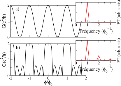
Figure 4: (color online) $a)$ Magnetoconductance of an ideal ring as a function of the magnetic field $\phi/\phi_{0}$. The Fourier transform (FT) of the magnetoconductance (in the inset) shows only the AB peak at freq. $\phi_{0}^{-1}$. $b)$ Magnetoconductance of a realistic ring in which the S matrix of Eq.(7) regulates the scattering of the electron at the leads. As a consequence of the backscattering, the FT of the magnetoconductance (inset) shows higher order frequencies.

In Fig.(4) we show the magnetoconductance of the ring in the absence of RSOI ($k_{SO}R=0$). In panel a) of Fig.(4), only the path of Fig. (1, $1a)$ has been considered, i.e., full transmission across the ring is assumed, as it would be the case for ideal coupling to the leads. The corresponding Fourier spectrum is showed in the corresponding inset. The well known Ahronov-Bohm sinusoidal pattern implies that just the fundamental frequency $\phi_{0}^{-1}$ appears.

To make the model more realistic, we allow for higher order looping of the electron within the ring. In Ref.noiletter , only the paths of the kind of Fig.(1,2a),1,2b)) were included. Here, we consider also the paths of the kind of Fig.(2) in which the electron can be backscattered at the leads. We use here $\bar{r}=0$ in the scattering matrix between the arms and the leads, which means that no backreflection in the incoming lead is present. The magnetoconductance of the ring, in this regime, is showed in Fig. (4b). Because of the inclusion of time reversed paths (TRP) within the ring, we see that higher order frequencies appear in the Fourier spectrum. In particular, the inset shows a peak at $2/\phi_{0}$ which is the signature of weak localizationnonloso .

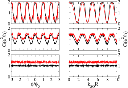
Figure 5: (color online)Conductance as a function of $\phi/\phi_{0}$ (left panels) and $k_{SO}R$ (right panels) for ideal (black curves) and realistic (red curves) contacts. An increasing amount of dephasing at the contacts is also included: from top to bottom: $\zeta=\pi/3,\pi,2\pi$

.

We also include some dephasing due to diffusiveness in the contacts by adding a random phase $z\in(-\zeta,\zeta)$ for each scattering at the leads. In Fig.(5), we report the conductance G vs. $\phi/\phi_{0}$ , with $k_{\text{SO}}R=0$ (left panels) or vs. $k_{SO}R$ with $\phi/\phi_{0}=0$ (right panels). These are averaged over $N=1000$ realizations of disorder, and plotted increasing the window of phase randomness ($\zeta=\pi/3,\pi,2\pi$ from top to bottom). The black curves refer to the case of Fig(4 $a)$) (ideal contacts) while the red curves refer to the case of realistic contacts (Fig(4 $b)$), with $\bar{r}=0$.

By comparing the top left panel of Fig.(5) with Fig.(4), we see that the ring is rather insensitive to small dephasing at the contacts. By increasing the amount of dephasing (middle and bottom left panels in Fig.(5)) we find that the sensitiveness is larger in the case of realistic contacts. This is due to the fact that for realistic coupling, the electrons in the ring can experience higher order paths, since it scatters with the leads many times.

In the right panel of Fig.(5), we plot the DC conductance vs. $k_{\text{SO}}R$ at $\phi/\phi_{0}=0$ for both ideal contacts and realistic contacts (and $\bar{r}=0$) (black and red lines in each box), with an increasing phase randomization (boxes from top to bottom with $\zeta=\pi/3,\pi,2\pi$), averaged over $N=1000$ realizations. In the case of ideal contacts and little dephasing (top right panel black curve), we see again the quasiperiodic oscillation of the conductance reproducing the localization conditions at the expected values of $k_{\text{SO}}R$ frustaglia ; molnar ; souma ; dario ; noiletter . When including higher order processes, interference effects give rise to a slightly different pattern. In the case of realistic contacts, we note that the device is seriously affected by dephasing, mainly because including the TRPs contributing to the transmission amplitude increases the number of scattering processes at the leads. Indeed, when the dephasing is quite large, it gives rise to random oscillations that are not averaged out, so that they wash out the conductance oscillations. The effect takes place for $\zeta\sim\pi$ when TRPs are included, in contrast to $\zeta\sim 2\pi$ when the TRPs are absent. As regular magnetoconductance oscillations are experimenally observed nitta ; yau ; morpurgo ; kato ; molenkamp with little precentage of contrast between maxima and minima, we conclude that, in real samples, dephasing is ubiquitous.

VIII Spin Transmission

In this Section we calculate the rotation of the spin of the electron transmitted through the ring. We first consider an incoming electron beam with in-plane spin polarization (let’s say, polarized along the $x$ direction ). The spin rotation is measured by calculating the average value of the outgoing spin:

$$\langle S_{z}\rangle=\frac{\left\langle\Psi_{out}\right|S_{z}\left|\Psi_{out}\right\rangle}{\left\langle\Psi_{out}\right.\left|\Psi_{out}\right\rangle}\;.$$ (49)

Since in the previous Section we have shown that higher order looping just adds subleading higher order harmonics to the conductance, here we focus on the case of ideal contacts, that is, we include in the calculation only paths as the ones of Fig.(1,1a). The in plane polarization can be considered as a superposition of equal weighted z-polarized spin components. In the absence of RSOI ($k_{SO}R=0$), opposite spin polarizations do not interfere with each other. As a consequence, the total expected $\langle S_{z}\rangle$ component keeps zero at the exit. Fig.(6) shows the magnetoconductance for increasing $k_{SO}R$, and the corresponding expected spin component polarized along the $z-$axis at the exit of the ring. The Zeeman term is on the diagonal of the spin Hamiltonian of Eq.(31) and operates to keep the $z-$components of the spin polarization fixed, while the RSOI is offdiagonal and tends to favor inplane spin polarization. This implies that when the magnetic field increases ($\phi/\phi_{0}>>k_{SO}R$) the spin polarization gets frozen to the incoming polarization. This is the reason why,in Fig.(6), at high fields, the trasmitted spin polarization is inplane. Incidentally we observe that this result should not be expected in real systems in which spin relaxation can occur due to electron-phonon interaction or other mechanisms as hyperfine interaction with nuclear spins. Spin relaxation would induce flipping of that spin component that is energetically unfavourable and the final transmission of the spin will result to be partly out of the $x-y$ plane. On the contrary, when $\phi/\phi_{0}\sim k_{SO}R$ the competition of the Zeeman and the RSOI induces a coherent rotation of the spin while the electron travels along the ring. Fig.(6) shows that, when $\phi/\phi_{0}\sim k_{SO}R$, the spin is moved significantly out of the $x-y$ plane, consistently affecting the AB oscillations.

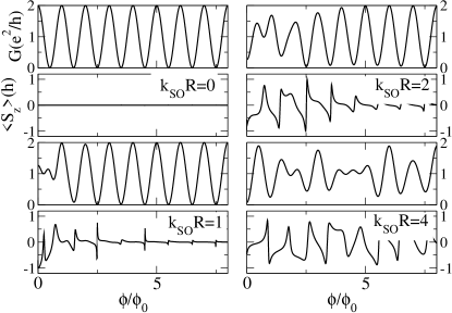
Figure 6: Magnetoconductance and expectation value of the outgoing $\hat{z}$ spin component for an incoming spin in the $x$ direction at different values of the RSOI strength ($k_{SO}R=0,1,2,4$ indicated in the pictures).

To better understand what happens when $\phi/\phi_{0}\sim k_{SO}R$, we isolate the spin “up” polarization for the incoming particle in what follows ($\left\langle\Psi_{in}\right|S_{z}\left|\Psi_{in}\right\rangle/\left\langle\Psi_{in}\right.\left|\Psi_{in}\right\rangle=1$) and we separately plot in Fig.(7) the two contributions to the conductance $G_{up-up}$ (full line) and $G_{down-up}$ (dotted line), for opposite polarizations of the outgoing electron. $G_{up-up}$ is the contribution to the conductance arising from the particle flux that mantains the same polarization at the exit as the incoming one, while $G_{down-up}$ refers to a particle flux having the opposite polarizations at the exit with respect to the one at the entrance. Of course, when $k_{SO}R=0$, the electron spin is in the “up”direction for any $\phi/\phi_{0}$. When both RSOI and magnetic field are present, with $\phi/\phi_{0}>>k_{SO}R$, the spin polarization is steadly in the $z-$ direction, except for sharp reversals at flux values $\phi_{0}m/2$ ($m$ integer). However, $G_{down-up}$ is vanishingly small at these places, together with $G_{up-up}$. Therefore the conductance vanishes at these points anyhow, and the transmitted spin polarization is fully up, except for these points. On the contrary, in the parameter intervals characterized by $\phi/\phi_{0}\sim k_{SO}R$, both $G_{up-up}$ and $G_{down-up}$ are non vanishing (see Fig.7), so that the spin is rotated at the exit, with nonvanishing transmission amplitude.

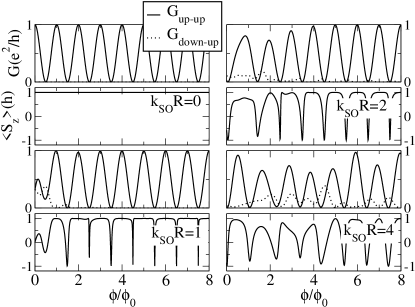
Figure 7: Separate contributions to the magnetoconductance for different outcoming spin polarizations, $G_{up-up}$ (full line) and $G_{down-up}$ (dotted line ) compared to the expected value of the outgoing $\hat{z}$ spin component. The incoming spin is polarized “up” . Different values of the RSOI strength are reported ($k_{SO}R=0,1,2,4$ indicated in the picture ).

We now examine in more detail the expected dependence of the outgoing spin polarization on the RSOI, at zero magnetic field. For an incoming electron polarized with spin “up”, Fig.(8(a)) shows that a large enough RSOI produces a rotation of the spin which points down at the exit for any $k_{SO}R$ value. Meanwhile, the total conductance oscillates with $k_{SO}R$. This finding also appears in Ref.souma and is quite remarkable, because it is the consequence of the interference between the two arms of the ring. In order to point out the role of quantum interference, we discuss here, for comparison, what happens by transporting a spinful electron along a single arm of the ring (the upper one). When just one arm is considered, (see Fig(8b)) spin polarization oscillates, as a function of $k_{SO}R$ datta , while the conductance is always unitary, because of the conservation of the particle flux. In the limit of large $k_{SO}R$ the propagation amplitude for the travelling electron acquires a simple analytical form. From Eq.(47) we see that, in the representation of the instantaneous spin eigenvectors, the spin propagator at the exit time $t_{f}$ (with $\omega_{o}t_{f}=\pi)$, in this limit is diagonal:

$$U^{u\rightarrow}(t_{f},0)=\left(\begin{array}[]{c c}ie^{-i\pi\gamma}&0\\ 0&-ie^{i\pi\gamma}\end{array}\right)\>\>,$$ (50)

so that the spin appears not to be rotated at the exit in the rotating reference frame. However, in order to move from the representation of the instantaneous spin eigenvectors to the reference basis, one has to perform the transformation with the unitary $B$ matrix of Eq.(40) , with $\vartheta=\pi/2$. The spin part of the propagator for an electron travelling into the upper arm (upper path of Fig.(1,1a)) is then:

$$U^{u\rightarrow}_{spin}(t_{f},0)=B(t_{f})U^{u\rightarrow}(t_{f},0)B^{\dagger}(0)$$

$$=\left(\begin{array}[]{c c}i\cos(\pi\gamma)&\sin(\pi\gamma)\\ -\sin(\pi\gamma)&-i\cos(\pi\gamma)\end{array}\right)\>\>.$$ (53)

If we inject $up$ electrons in the upper arm only, the expectation value of the the outcoming $S_{z}$ defined in Eq.(49) is: $\langle S_{z}\rangle=\cos(2\pi\gamma)=\cos(\pi k_{SO}R)$ (note that for large enough $\gamma$ this result well approximates the red-full line in Fig.(8b)). The conductance is unitary, $G=2e^{2}/h$ (the black-dashed line in Fig.(8b), as no interference takes place.

We now go back to the transmission along both arms simultaneously and examine the resulting interference. According to the rules given after Eq.(47), in the same limiting case as above, the propagator accounting for transmission of incoming $up$ spins across the ring is:

$$U^{u\rightarrow+d\rightarrow}_{spin}(t_{f},0)=\left(\begin{array}[]{c c}0&2\sin(\pi\gamma)\\ -2\sin(\pi\gamma)&0\end{array}\right)\>\>,$$ (54)

so that the spin at the exit is reversed. In fact, in the expectation value of Eq.(49), the oscillations in the numerator compensate those in the denominator, eventually giving $\langle S_{z}\rangle=-1$ (for large enough $\gamma$ this result well approximate the red-full line in Fig.(8a)). The conductance however oscillates according to $G/(2e^{2}/h)=2\sin^{2}(\pi k_{SO}R/2)$, as plotted in the black-dashed line in (Fig.8a)).

It is quite remarkable that this result is only found at zero magnetic field. Indeed, no matter how small $B$ is, the time reversal symmetry is broken and the spin oscillates with $k_{SO}R$ (see Fig.(9,a). However, for very small magnetic field these oscillations are confined close to special values of $k_{SO}R=2l$($l$ integer) and display a Lorentzian shape around these points. The role of the magnetic field is to make the oscillations broader.

To summarize, there are two limiting conditions in the outgoing spin polarization, for incoming “up” spin polarization: $a)$ the zero RSOI which leaves the incoming spin polarization unchanged, provided no relaxation takes place; $b)$ the zero magnetic flux case in which the RSOI produces a flip of the spin at the exit. It is interesting that when the flux $\phi$ is an integer number of flux quanta $\phi_{0}$, the crossover between case $a)$ and case $b)$, with $k_{SO}R$ increasing from the value zero to values $k_{SO}R>>\phi/\phi_{0}$ is rather sharp. This is shown in Fig. (9,b) where the expectation value of the outcoming spin is plotted vs. $k_{SO}R$ for different integer values of $\phi/\phi_{0}$. For values of $\phi/\phi_{0}>>k_{SO}R$ the outgoing spin polarization is the same as that at the entrance, ( $up$ in the picture). On the contrary, by increasing $k_{SO}R$ at non zero $B$ field, we see again a pattern similar to the one of Fig. (9,a), but shifted to higher values of $k_{SO}R$.

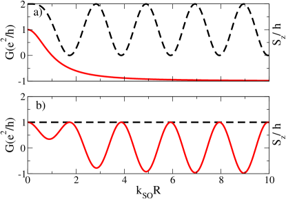
Figure 8: (color online) Conductance (broken line) and spin polarization (full line) of the outgoing electron for $B=0$, as a function of the RSOI. The spin of the incoming electrons is polarized “$up$” : $a)$ The ring case with ideal contacts. $b)$ a single wire of the same length and curvature as one of the ring arms.

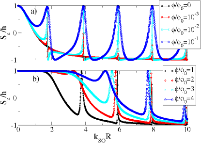
Figure 9: (color online) Expectation value of the outgoing spin for incoming spin “$up$” polarized electrons as a function of the RSOI for different values of the magnetic flux : $a)$ $\phi/\phi_{0}$ zero or very small; $b)$ increasing integer values of $\phi/\phi_{0}$.

IX Conclusions

To conclude, we have employed a path integral real time approach to compute the DC conductance of a ballistic one dimensional mesoscopic ring in both external electrical and magnetic fields orthogonal to the ring plane.The spinful electron experiences a Rashba spin orbit interaction and the Zeeman term. We employ a piecewise saddle point approximation for the orbital motion, but we implement the full scattering matrix at the leads and sum over all the possible higher order paths up to convergency of the result. Our approach goes beyond other recent semiclassical calculations. Our theory is nonperturbative and separates the adiabatic spin dynamics from the non adiabatic one by using the rotating frame for the spin travelling around the ring. In practice, we diagonalize the time dependent spin Hamiltonian in the representation of the spin eigenvectors of the instantaneous Hamiltonian. This allows us to explore a wide range of Hamiltonian parameters, ranging from the limit of strong magnetic field and weak Rashba SOI to the opposite case. In both extreme regimes our piecewise saddle point approximation is very efficient as quantum fluctuations with flipping of the spin has little influence on the orbital motion. This is also seen from the number of paths required to gain full convergency. As explained in Sec. $V$ the separation of adiabatic from non adiabatic spin dynamics shows that in the intermediate regimes our approximation is less justified, but nevertheless, the results it produces seem to be in rather good agreement with recent numerical calculations frustaglia ; molnar ; shen ; dario ; souma and experimentsnitta ; yau ; morpurgo ; kato ; molenkamp . When we include also time reversed paths, the Fourier transform of the magnetoconductance shows the typical $\phi_{0}/2$ peak due to weak localizationnonloso .This would be the only surviving contribution if an ensemble average or different rings were measuredkoga .

We have also allowed for nonideal couplings between ring and leads as we account for dephasing effects due to diffusiveness at the contacts. The results satisfactorily compare with experiments where the contrast between maxima and minima in the interference fringes is always few tens of percentage of the background DC signal.

Appendix A Motion of a classical spin in a rotating magnetic field

In this appendix we derive the classical equations of motion for the spin from the Lagrangian in Eq.(14), by assuming for the orbital coordinate the saddle point solution $\dot{\varphi}$ = constant. Once the orbital motion is dealt with in this way, the Lagrangian for the spin degrees of freedom is given by (besides a constant contribution)

$$\tilde{\cal L}[\Theta,\Phi,\dot{\Phi}]/\hbar=\left(\frac{1-\cos\Theta}{2}\right)\dot{\Phi}+\vec{{\cal B}}\cdot\vec{S}\>\>\>\>,$$ (55)

where the effective time dependent magnetic field is ${\cal{B}}\equiv({\cal{B}}_{+},{\cal{B}}_{-},{\cal{B}}_{z})=\left(\gamma\dot{\varphi}\>e^{i\varphi},\gamma\dot{\varphi}\>e^{-i\varphi},-\omega_{c}/2\right)$. To derive the equations of motion from a variational principle, we write the Berry phase term in the total spin action as

$$\tilde{S}_{B}=\int_{\Phi(0)}^{\Phi(t_{f})}\>dt\>\left(\frac{1-\cos\Theta}{2}\right)d\Phi=\int_{\Sigma}\sin\Theta\>d\Theta\wedge d\Phi\>\>\>\>,$$ (56)

where $\Sigma$ is the spherical triangle with vertices given by the north pole on the sphere and by the points with coordinates $(\Theta(0),\Phi(0))$ , $(\Theta(t_{f}),\Phi(t_{f}))$. Let $(t,u)$ be a parametrization of the spherical triangle, such that $\vec{S}(t,1)=\vec{S}(t)$, and $\vec{S}(t,0)=(0,0,1)$. Thus, one may rewrite the action $\tilde{S}_{B}$ in Eq.(56) as

$$\tilde{S}_{B}=\int_{0}^{T}\>dt\>\int_{0}^{1}\>du\>{\bf S}\cdot\left[\frac{\partial{\bf S}}{\partial t}\times\frac{\partial{\bf S}}{\partial u}\right]\>\>\>\>.$$ (57)

To derive the equations of motion, we consider a variation $\vec{S}(t,u)\rightarrow\vec{S}(t,u)+\delta\vec{S}(t,u)$ such that $\vec{S}(T,u)$ and $\vec{S}(0,u)$ are ”locked”, that is, $\delta\vec{S}(0,u)=\delta\vec{S}(T,u)=0$. Since $[\vec{S}(t,u)]^{2}=1$ $\forall t,u$, one gets $\vec{S}\cdot\frac{\partial\vec{S}}{\partial t}=\vec{S}\cdot\frac{\partial\vec{S}}{\partial u}=0$, As a consequence, $\frac{\partial\vec{S}}{\partial t}\times\frac{\partial\vec{S}}{\partial u}$ is parallel to $\vec{S}$. As $\delta\vec{S}\cdot\vec{S}=0$, this implies that

$$\int_{0}^{T}\>dt\>\int_{0}^{1}\>du\>\delta\vec{S}\cdot\left[\frac{\partial\vec{S}}{\partial t}\times\frac{\partial\vec{S}}{\partial u}\right]=0\>\>\>\>.$$ (58)

Thus, by integrating by parts we see that the only nonzero variation of $\tilde{S}_{B}$ is given by the boundary term

$$\delta\tilde{S}_{B}=\int_{0}^{t_{f}}\>dt\>\delta\vec{S}(t)\cdot\left[\vec{S}(t)\times\frac{\partial\vec{S}(t)}{\partial t}\right]\>\>\>\>,$$ (59)

where we have used the fact that $\vec{S}(t,1)=\vec{S}(t)$. By equating to zero the total variation of the action, one obtains

$$\vec{S}\times\frac{d\vec{S}}{dt}=\vec{\mathcal{B}}\>\>\>\>,$$ (60)

that is, the classical equations of motion we used in section IV. To show that Eqs.(60), when the spin components are expressed in polar coordinates, are equivalent to Eqs.(17,18), let us set $\omega=\gamma\dot{\varphi}$ and $\Omega=-\omega_{c}/2$. Also, we define

$$S_{+}=S_{x}+iS_{y}\hskip 56.9055pt{\mathcal{B}}_{+}={\mathcal{B}}_{x}+i{\mathcal{B}}_{y}$$

$$S_{-}=S_{x}-iS_{y}\hskip 56.9055pt{\mathcal{B}}_{-}={\mathcal{B}}_{x}-i{\mathcal{B}}_{y}\vspace*{1cm}\>\>\>\>.$$

In terms of the new variables, the equations of motion are given by

$$\frac{dS_{z}}{dt}=\frac{i}{2}({\mathcal{B}}_{+}S_{-}-{\mathcal{B}}_{-}S_{+})$$

$$\frac{dS_{+}}{dt}=i({\mathcal{B}}_{z}S_{+}-{\mathcal{B}}_{+}S_{z})$$

$$\frac{dS_{-}}{dt}=-i({\mathcal{B}}_{z}S_{-}-{\mathcal{B}}_{-}S_{z})\>\>\>\>.$$ (61)

or:

$$\frac{dm(t)}{dt}=i\>\left(\Omega-\dot{\varphi}\right)\>p(t)-2\>i\omega\>S_{z}$$

$$\frac{dp(t)}{dt}=i\>\left(\Omega-\dot{\varphi}\right)\>m(t)$$

$$\frac{dS_{z}}{dt}=-\frac{i\omega}{2}\>{m(t)}\>$$ (62)

where

$$p(t)=S_{+}e^{(-i\varphi)}+S_{-}e^{(i\varphi)}$$

$$m(t)=S_{+}e^{(-i\varphi)}-S_{-}e^{(i\varphi)}\>\>\>\>,$$

and $1=4|S|^{2}=4{S_{z}}^{2}+(p^{2}-m^{2})$. By introducing $b=\Omega-\dot{\varphi}$, we obtain:

$$\frac{d(m(t)+p(t))}{dt} = ib\left(m(t)+p(t)\right)-2i\omega\>S_{z}(t)$$ (63)

$$\frac{d{S}_{z}(t)}{dt} = -i\omega\>m(t)$$ (64)

Resorting to the polar coordinates $(\Theta,\Phi)$ for the spin $\vec{S}$, we get:

$$\left[\dot{\Theta}\cos\Theta+i\left(\dot{\Phi}-\Omega\right)\sin\Theta\right]e^{i\chi}+i\cos\Theta\alpha\dot{\varphi}=0$$ (65)

$$\left[\dot{\Theta}-\omega\>\sin{\chi}\right]\sin\Theta=0\>\>\>\>.$$ (66)

Eq.(66) is the same as Eq.(17). The real part of Eq.(65) is proportional to the imaginary part: both give Eq.(18) when equated to zero, which completes the proof.

Appendix B The spin propagator

In order to find the propagator of the Berry Hamiltonian $\hat{H}_{A}$ of Eq.(45), we solve the system of differential Eq.(42), in the representation of the instantaneous eigenvectors:

$$i\frac{d}{dt}\left(\begin{array}[]{c}u_{+}\\ u_{-}\end{array}\right)\>=\left(\begin{array}[]{cc}r+\omega_{o}\sin^{2}\frac{\vartheta}{2}&\omega_{o}\sin\frac{\vartheta}{2}\cos\frac{\vartheta}{2}e^{-i\omega_{o}t}\\ \omega_{o}\sin\frac{\vartheta}{2}\cos\frac{\vartheta}{2}e^{i\omega_{o}t}&-r-\omega_{o}\sin^{2}\frac{\vartheta}{2}\end{array}\right)\left(\begin{array}[]{c}u_{+}\\ u_{-}\end{array}\right)\>\>\>\>.$$ (67)

To solve Eq.(67), first of all, we switch to a time-independent coefficient matrix by defining:

$$\left(\begin{array}[]{c}y_{+}\\ y_{-}\end{array}\right)\>=\left(\begin{array}[]{cc}e^{+i\frac{\omega_{o}}{2}t}&0\\ 0&e^{-i\frac{\omega_{o}}{2}t}\end{array}\right)\left(\begin{array}[]{c}u_{+}\\ u_{-}\end{array}\right)\>.$$ (68)

By setting

$$Y=\left(\begin{array}[]{c}y_{+}\\ y_{-}\end{array}\right)\>\>\>;\>\>W=\left(\begin{array}[]{c}u_{+}\\ u_{-}\end{array}\right)\>,$$

we define the matrix $T$ through

$$Y\>=\>T\>W,\;\;\;W\>=\>T^{-1}\>Y\>.$$ (69)

Eqs.(67) now read:

$$i\frac{dy_{+}}{dt}(t)=(r-\frac{\omega_{o}}{2}cos(\vartheta))y_{+}(t)+\frac{\omega_{o}}{2}\sin\vartheta y_{-}(t)\>,$$

$$i\frac{dy_{-}}{dt}(t)=+\frac{\omega_{o}}{2}\sin\vartheta y_{+}(t)+(-r+\frac{\omega_{o}}{2}cos(\vartheta))y_{-}(t)\>.$$ (70)

Now we define $r^{\prime}=r-\frac{\omega_{o}}{2}\cos\vartheta$ and $s=\frac{\omega_{o}}{2}\sin\vartheta$, so that in matrix form we have:

$$i\frac{d}{dt}\left(\begin{array}[]{c}y_{+}\\ y_{-}\end{array}\right)\>=\left(\begin{array}[]{cc}r^{\prime}&s\\ s&-r^{\prime}\end{array}\right)\left(\begin{array}[]{c}y_{+}\\ y_{-}\end{array}\right)\>,$$ (77)

in a compact form we can rewrite the last equation as:

$$i\frac{d}{dt}Y\>=\>C\>Y\>,$$ (78)

which defines the matrix $C$.
We now decouple the previous system of equation by diagonalizing the matrix $C$. Its eigenvalues are $\lambda=\pm\epsilon=\pm\sqrt{r^{\prime 2}+s^{2}}$ and the matrix that diagonalizes $C$ is

$$P=\left(\begin{array}[]{cc}1&\frac{r^{\prime}-\epsilon}{s}\\ \frac{\epsilon-r^{\prime}}{s}&1\end{array}\right)\>.$$ (79)

Its inverse is

$$P^{-1}=\left(\begin{array}[]{cc}\frac{s^{2}}{2\epsilon(\epsilon-r^{\prime})}&\frac{(\epsilon-r^{\prime})s}{2\epsilon(\epsilon-r^{\prime})}\\ -\frac{(\epsilon-r^{\prime})s}{2\epsilon(\epsilon-r^{\prime})}&\frac{s^{2}}{2\epsilon(\epsilon-r^{\prime})}\end{array}\right)\>.$$ (80)

Eq.(78) now reads:

$$i\frac{d}{dt}P^{-1}\>Y\>=\>P^{-1}\>C\>P\>P^{-1}\>Y\>,$$ (81)

which, by defining $V\>=\>P^{-1}\>Y$, becomes

$$i\frac{d}{dt}V\>=\left(\begin{array}[]{cc}\epsilon&0\\ 0&-\epsilon\end{array}\right)\>V\>.$$ (82)

Its formal solution is:

$$V(t)\>=\left(\begin{array}[]{cc}e^{-i\epsilon(t-t^{\prime})}&0\\ 0&e^{i\epsilon(t-t^{\prime})}\end{array}\right)\>V(t^{\prime})\>,$$ (83)

or, in matrix form

$$V(t)\>=\>S(t-t^{\prime})\>V(t^{\prime})\>.$$ (84)

Now we apply inverse transformations, in order to obtain the full Schrödinger propagator, that is the matrix transformation between ($W(t^{\prime})$ and $W(t)$).

$$W(t)\>=\>T^{-1}(t)\>P\>S\>P^{-1}\>T(t^{\prime})\>W(t^{\prime})\;\;,$$

where $P$ is time independent. The full evolution operator in the adiabatic basis is:

$$U(t,t^{\prime})\>=\>T^{-1}(t)\>P\>S\>P^{-1}T(t^{\prime})\>;$$ (85)

By performing all the matrix products, we obtain the result of Eq.(47), as given in the text.

References

- (1) Y. Aharonov, D. Bohm, Phys. Rev. 115 485 (1959).
- (2) S. Washburn and R. A. Webb, Rep. Prog. Phys. 55, 1311 (1992).
- (3) J. Anandan, Science 297, 1656 (2002).
- (4) M. V. Berry, Proc. R. Soc. London, A 392, 45 (1984).
- (5) Y. Aharonov, J. Anandan, Phys. Rev. Lett. 58, 1593 (1987).
- (6) E.I. Rashba, Fiz. Tverd. Tela 2, 1224 (1960) [Sov.Phys. - Solid State 2, 1109 (1960),Y.A. Bychkov, E.I. Rashba, J.Phys.C17, 6039 (1984).
- (7) F. E. Meijer, A. F. Morpurgo, T. M. Klapwijk, T. Koga and J. Nitta, Phys. Rev. B 70 201307 (2004).
- (8) J. B. Miller, D. M. Zumbühl, C. M. Marcus, Y. B. Lyanda-Geller, D. Goldhaber-Gordon, K. Campman and A. C. Gossard, Phys. Rev. Lett. 90 076807 (2003).
- (9) A. G. Aronov and Y. L. Lyanda-Geller, Phys. Rev. Lett.70, 343 (1993).
- (10) Y.Ahronov and A. Casher Phys. Rev. Lett. 53, 319 (1984).
- (11) J. Nitta, T.Koga, F. E. Meijer, Physica E 18, 143 (2003); F. E. Meijer, J. Nitta, T. Koga, A.F. Morpurgo, T. M. Klapwijk, Physica E 22, 402, (2004); M.J. Yang, C.H. Yang, K.A. Cheng and Y.B. Lyanda-Geller, cond-mat/0208260.
- (12) J. B. Yau, E. P. de Poortere, and M. Shayegan, Phys. Rev. Lett. 88, 146801 (2002).
- (13) A. F. Morpurgo, J. P. Heida, T. M. Klapwijk, B. J. van Wees and G. Borghs, Phys. Rev. Lett. 80, 1050 (1998).
- (14) Y.K. Kato, R.C. Meyers, A.C. Gossard, D.D. Awshalom cond/mat 2005
- (15) M. König, A. Tschetschetkin, E.M. Henkiewicz, J. Sinova, V. Hock, V. Daumer, M. Schäfer, C.R. Becker, H. Buhmann and L.W. Molenkamp, Phys. Rev. Lett. 96 0760804 (2006).
- (16) R.Capozza, D.Giuliano, P. Lucignano, and A. Tagliacozzo, Phys. Rev. Lett. 95, 226803 (2005).
- (17) B. Habib, E. Tutuc and M. Shayegan cond-mat/0612638.
- (18) A review is given by C. W. J. Beenakker and H. van Houten, Solid State Phys., 44, 1 (1991).
- (19) D. Loss, P. Goldbart and A. V. Balatsky, Phys. Rev. Lett. 65, 1655 (1990); H. A. Engel and D. Loss, Phys. Rev. B 62, 10238 (2000).
- (20) R. P. Feynmann, Quantum Mechanics and Path Integral, Mc Graw-Hill, New York 1965.
- (21) Y. Tserkovnyak and A. Brataas cond-mat/0611086
- (22) D. Frustaglia, K. Richter, Phys. Rev. B 69 235310 (2004).
- (23) B. Molnár, F. M. Peeters and P. Vasilopoulos, Phys. Rev. B 69, 155335 (2004); X.F.Wang and P. Vasilopoulos Phys. Rev. B 72, 165336 (2005).
- (24) S.Q. Shen, Z.J. Li and Z. Ma, Appl. Phys. Lett. B 84, 996 (2004).
- (25) D.Becioux, D.Frustaglia and M.Governale, Phys. Rev. B 72, 113310 (2005).
- (26) R. Citro, F. Romeo and M. Marinaro Phys. Rev. B 74, 115329 (2006).
- (27) S.Souma and B.K.Nikolić, Phys.Rev.B70,195346(2004).
- (28) G.S. Lozano, M.J. Sanchez, Phys. Rev. B 72, 205315 (2005).
- (29) B.H. Wu and J.C. Chao, Phys. Rev. B 74, 115313 (2006)
- (30) R. Landauer, IBM J. Res. Dev.1 223 (1957); M. Buttiker, IBM J. Res. Dev.32 317 (1988).
- (31) F. D. M. Haldane Phys. Rev. Lett. 50, 1153 (1983).
- (32) M. Pletyukhov, Ch. Amann, M. Metha and M. Brack, Phys. Rev. Lett. 89 , 116601 (2002); O.Zaitsev, D. Frustaglia and K. Richter, Phys. Rev. Lett. 94, 026809 (2005).
- (33) C. Morette-de Witt, A. Maheshwari and B. Nelson, Phys. Rep. 50, 55 (1979).
- (34) In the current notation
- (35) G. Morandi and E. Menossi, Eur. J. Phys. 5 49 (1984).
- (36) A. Aurbach, F. Berruto and L. Capriotti, Field theory for low-dimensional systems Ed.s G. Morandi, P.Sodano, A.Tagliacozzo and V.Tognetti (Springer New York 2000).
- (37) S. Datta and B. Das, Appl. Phys. Lett. 56, 665 (1990).
- (38) T.Koga, Y.Sekine and J.Nitta, Phys.Rev.B74, 041302 (2006).