Stationary spatial structures in reaction-subdiffusion

Abstract

We discuss stationary concentrations of reactants in an $\mathrm{A}+\mathrm{B}\rightarrow 0$ reaction under subdiffusion and show that they are described by stationary reaction-diffusion equations with a nonlinear diffusion term. We consider stationary profiles of reactants’ concentrations and of reaction zones in a flat subdiffusive medium fed by reactants of both types on its both sides (a subdiffusive gel reactor). The behavior of the concentrations and of the reaction intensity in subdiffusion differs strikingly from those in simple diffusion. The most important differences correspond to the existence of accumulation and depletion zones close to the boundaries and to non-monotonous behavior of the reaction intensity with respect to the strength of the minor source. The implications of these results for other situations are also discussed.

Many phenomena in systems out of equilibrium are described as reactions between diffusing species. Apart from chemistry, examples are trapping and annihilation of excitons or recombination of charge carriers in physics, or predator-prey relations in ecology. For normal diffusion the situation is described in terms of reaction-diffusion equations. Many systems however exhibit anomalous diffusion with a mean square displacement scaling as $\left<r^{2}(t)\right>\propto t^{\alpha}$, with $0<\alpha<1$ in the subdiffusive case and $\alpha>1$ in the superdiffusive case, which is not described by a diffusion equation Phys2day ; PhysWorld . Subdiffusion can often be modeled within the framework of continuous time random walks (CTRW) with a heavy-tailed waiting time density function $\psi(t)\propto t^{-1-\alpha}$, which yields a fractional subdiffusion equation. In analogy to reaction-diffusion, fractional reaction-subdiffusion equations have been proposed, where an additional fractional time derivative acts either on the spacial Laplacian Wearnes ; Koszt or on both the spatial Laplacian and the reaction term YAK ; SWT . Refs.SSS1 ; SSS2 showed that the reaction-subdiffusion equations do not follow by simply changing a diffusion operator in a reaction-diffusion equation for a subdiffusion one. The situation here was pertinent to initial-condition problems. A rather general approach to reaction-subdiffusion equations was proposed in Ref.horsthemke , where, after deriving the set of reaction-subdiffusion equations the authors analyzed the properties of Turing instability in corresponding reaction-subdiffusion systems. In what follows we discuss the simplest boundary condition problem in which nontrivial stationary spacial structures appear, namely the irreversible $\mathrm{A}+\mathrm{B}\rightarrow 0$ reaction YAK , and focus on stationary concentration profiles under given, steady concentrations of reactants on the boundaries (Ref.YAK started with one reactant, A or B, on each side). We show that the spacial structures under reaction-subdiffusion are strikingly different from ones emerging in reaction-diffusion. We first give the derivation of subdiffusion-reaction equations and stationary subdiffusion-reaction equations by generalizing the scheme put forward in Refs.SSS1 ; SSS2 . As in horsthemke , subdiffusion is considered within a CTRW scheme, and the reaction locally follows the mass action law. We then proceed by discussion of stationary forms of concentrations’ distributions and of those of reaction zones.

In a CTRW a particle arriving at a site $i$ at time $t^{\prime}$ stays there for a sojourn time $t$, which is given by the probability density function $\psi(t)$. Leaving the site it makes a step with probability 1/2 in either direction. In the following discussion we confine ourselves to the one-dimensional situation, however the generalization to whatever other geometry is quite evident.

The generalized reaction-diffusion equations are based on two balance conditions. The balance equation for A-particles at each site reads:

$$\dot{A}_{i}(t)=j_{i}^{+}(t)-j_{i}^{-}(t)+R_{i}\{A,B\}$$ (1)

$$=\frac{1}{2}j_{i-1}^{-}(t)+\frac{1}{2}j_{i+1}^{-}(t)-j_{i}^{-}(t)+R_{i}\{A,B\}.$$ (2)

where $j_{i}^{-}(t)$ is the loss flux of A-particles at site $i$, i.e. the probability for an A-particle to leave $i$ per unit time, $j_{i}^{+}(t)$ is the gain flux at the site, and $R_{i}\{A,B\}=-kA_{i}B_{i}$ is a reaction term, describing particles’ loss due to reaction. Since in our case the equations for A and B particles are symmetric, we concentrate on the equations for the A particles. A generalized reaction-diffusion equation is a combination of the continuity equation, Eq.(2), and the equation for the loss fluxes $j^{-}(t)$ following from the assumption about the distribution of sojourn times $\psi(t)$ and survival probability $P(t,t_{0})$.

According to the sojourn time distribution, the loss current for site $i$ at time $t$ is connected to the gain current for the site at all previous times and with the survival probability. Namely, the particles which leave site $i$ at time $t$ (making a step from $i$ to one of its neighbors) were either at site $i$ from the very beginning (and survived), or arrived there at some time $t^{\prime}<t$ and survived until $t$. The probability density to make a step at time $t$, having arrived at $t^{\prime}$, is given by the waiting time distribution $\psi(t-t^{\prime})$. We have then $j^{-}(t)=\psi(t)P_{i}(t,0)A_{i}(0)+\int_{0}^{t}\psi(t-t^{\prime})P_{i}(t,t^{\prime})j_{i}^{+}(t^{\prime})dt^{\prime}$, which, by using Eq.(1), can be rewritten in the form

$$j_{i}^{-}(t)=\psi(t)P_{i}(t,0)A_{i}(0)+\int_{0}^{t}\psi(t-t^{\prime})P_{i}(t,t^{\prime})\times$$

$$\times\left[\dot{A}_{i}(t^{\prime})+j_{i}^{-}(t^{\prime})+kA_{i}(t^{\prime})B_{i}(t^{\prime})\right]dt^{\prime}.$$ (3)

The survival probability of A at $i$ is given by the classical kinetic equation $\frac{d}{dt}P_{i}(t)=-kB_{i}(t)P_{i}(t)$ and depends on the time-dependent B-concentration via

$$P_{i}(t,t_{0})=\exp\left(-k\int_{t_{0}}^{t}B_{i}(t^{\prime})dt^{\prime}\right).$$ (4)

At this stage we also can assume the concentrations to be slowly changing is space, and change to a continuous coordinate $x=ai$, with $a$ being the lattice spacing:

$$\dot{A}(x,t)=\frac{a^{2}}{2}\Delta j^{-}(x,t)-kA(x,t)B(x,t).$$ (5)

Eq.(5) together with Eqs.(3) and (4) and their counterparts for B-concentration give us the full system of equations for time-dependent concentrations. This system can be transformed to a special case of reaction-subdiffusion equations considered in Ref. horsthemke . However, at this stage it is easier to proceed with the equations in our form.

In our previous discussion we considered an initial condition problem, where A-particles were introduced at time $t=0$ into the system and followed the evolution of their concentration. In the case of normal diffusion the situation in steady state (achieved, say, if the concentration of the particles at boundaries of the system is fixed by external sources) is given by the same reaction-diffusion equations, with the time derivatives at the left hand side put to zero. For the case of subdiffusion the situation is a bit more involved.

Let us assume that in the course of time the system achieves a steady state characterized by constant concentrations $A(x)$ and $B(x)$. Such a steady state is maintained through the particles’ sources at the boundaries of the system, no particle sources exist in the interior. Let us label the particles according to the time $t_{0}$ they were introduced into the system, so that e.g. $A(x,t|t_{0})dt_{0}$ is the concentration at point $x$ at time $t$ of A-particles introduced between $t_{0}$ and $t_{0}+dt_{0}$ (a partial concentration of A). The partial concentration $A(x,t_{0}|t_{0})$ of newly introduced particles is zero everywhere in the interior of the system. The overall concentration of A-particles at site $x$ is given by the integral

$$A(x)=\int_{-\infty}^{t}A(x,t|t_{0})dt_{0}.$$ (6)

In a steady state $A(x,t|t_{0})$ can only be a function of the difference of the time-arguments, i.e. of the elapsed time $t_{e}=t-t_{0}$ so that $A(x,t|t_{0})=A(x,t-t_{0})$ and the equations for the partial concentrations $A(x,t|t_{0})$ are given by Eqs.(5) with $t$ changed to $t_{e}$. Moreover, the overall concentration $A(x)$ is given by $A(x)=\int_{0}^{\infty}A(x,t_{e})dt_{e}$. Since $A(x)$ and $B(x)$ are time-independent, the survival probabilities $P_{A}(x,t,t^{\prime})$ and $P_{B}(x,t,t^{\prime})$ in reaction-subdiffusion equations are the functions of the differences of their time-arguments so that $P_{A}(x,t,t^{\prime})=\exp\left[-kB(x)(t-t^{\prime})\right]$. The integral in the equation for the flux now takes the form of a convolution:

$$j^{-}(x,t|t_{0})=\psi(t)P_{A}(x,t-t_{0})A(x,t_{0}|t_{0})$$

$$+\int_{t_{0}}^{t}\psi(t-t^{\prime})P_{A}(x,t-t^{\prime})\times$$ (7)

$$\times\left[\dot{A}(x,t^{\prime}|t_{0})+j^{-}(x,t^{\prime}|t_{0})+kA(x,t^{\prime}|t_{0})B(x)\right]dt^{\prime}$$

where $j^{-}(x,t^{\prime}|t_{0})$ are the loss fluxes for those A-particles which were introduced into the system at time $t_{0}$. We now pass to the Laplace domain with respect to $t_{e}$ and denote $\tilde{A}(x,u)=\int_{t_{0}}^{\infty}A(x,t|t_{0})\exp[-u(t-t_{0})]dt$. The Laplace transform of the product $\Psi(t,x)=\psi(t)\exp\left[-kB(x)t\right]$ is given by the shift theorem and is equal to $\tilde{\Psi}(u,x)=\tilde{\psi}(u+kB(x))$, so that

$$\tilde{j}^{-}(x,u)=\frac{[u+kB(x)]\tilde{\psi}(u+kB(x))}{1-\tilde{\psi}(u+kB(x))}\tilde{A}(x,u).$$ (8)

Inserting this into the first equation we get in the Laplace domain

$$u\tilde{A}(x,u)-A(x,t_{0}|t_{0})=$$ (9)

$$\frac{a^{2}}{2}\Delta\frac{[u+kB(x)]\tilde{\psi}(u+kB(x))}{1-\tilde{\psi}(u+kB(x))}\tilde{A}(x,u)-k\tilde{A}(x,u)B(x),$$

where $A(x,t_{0}|t_{0})$ differs from zero only at the boundaries. With $A(x)=\tilde{A}(x,0)$ the stationary concentration $A(x)$ in the interior of the system is given by

$$\frac{a^{2}}{2}\Delta\frac{kB(x)\tilde{\psi}(kB(x))}{1-\tilde{\psi}(kB(x))}A(x)-kA(x)B(x)=0,$$ (10)

with the boundary conditions corresponding to the given concentrations on the boundaries. For a Markovian case of regular diffusion, corresponding to $\psi(t)=\tau^{-1}\exp(-t/\tau)$, one has $\tilde{\psi}(u)=1/(1+u\tau)$ so that this equation reduces to $(a^{2}/2\tau)\Delta A(x)-kA(x)B(x)=0$, a usual stationary reaction-diffusion equation. In the non-Markovian case, corresponding to subdiffusion, the waiting time distribution in the Laplace domain is $\tilde{\psi}(u)\simeq 1-(\tau u)^{\alpha}\Gamma(1-\alpha)$ for small $u$ and Eq.(10) reads

$$\frac{a^{2}}{2}\frac{1}{\tau^{\alpha}\Gamma(1-\alpha)}\Delta B(x)^{1-\alpha}A(x)-k^{\alpha}A(x)B(x)=0.$$ (11)

It is easy to see that the Markovian equation is a special case of Eq.(11) for $\alpha=1$. The combination $D_{\alpha}=a^{2}/2\tau^{\alpha}\Gamma(1-\alpha)$ stands for a (generalized) diffusion coefficient. The full system of steady state equations is given by Eq.(10) and the corresponding equation for B. It is interesting to stress that the system of equations with additional temporal operator acting on the Laplacian in the case of initial-condition problem turns to a system of nonlinear reaction-diffusion equations with nonlinearity in the diffusion term for a stationary boundary-condition problem.

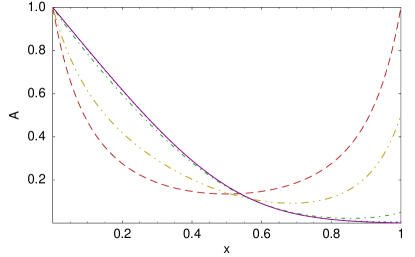
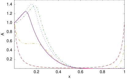
Figure 1: Stationary particle concentration profile $A(x)$ for $\alpha=1$ (upper panel) and for $\alpha=0.9$ (lower panel); $A(1)=1$ (dashed), $0.5$ (dash-dot-dot), $5\cdot 10^{-2}$ (dash-dot), $5\cdot 10^{-3}$ (dotted), and $1\cdot 10^{-4}$ (solid line), see text for details. Note the growth of the peak and its subsequent decay and outwards motion with decreasing minor source strength for the subdiffusive case; the behavior of the particle concentration profile in regular diffusion is monotonous with respect to the strength of the minor source and tends to a limiting form for $A(1)\rightarrow 0$.

As an example we consider a system on an interval $(0,1)$ with given reactants’ concentrations on the boundaries of the interval. The physical system we have in mind is a gel reactor or a porous medium in contact with two well-mixed reservoirs on both sides. The concentrations $A(0)=B(1)=1$ at the major sources are fixed. For the sake of simplicity we consider here symmetric situation with $A(0)=B(1)$ and $A(1)=B(0)$. Due to symmetry the $B$-concentration is then always symmetric to the $A$-concentration, i.e. $B(x)=A(1-x)$. The concentration $B(0)=A(1)$ will be called the minor source strengths (except for the symmetric case $A(1)=B(0)=1$). In Fig.1 we show numerical results for the steady-state Eqs.(11) obtained by semi-implicit relaxation algorithm. The results for subdiffusion (here with moderate $\alpha=0.9$) are compared to the ones for normal diffusion ($\alpha=1$ and hence linear diffusion operator). Shown is the behavior of the A-concentrations and the one of the reaction intensity $kA(x)B(x)$. The parameters are: $k=0.01$, $D_{\alpha}=1/2\Gamma(1-\alpha)$ for $\alpha=0.9$ and $D_{\alpha}=1/2$ for $\alpha=1$. The $A(0)=B(1)$ concentration is fixed to be $A(0)=1$, the other concentration varies from $B(0)=A(1)=1$ (symmetric case, when the CTRW-reactor separates two stoichiometric reacting mixtures) to $B(0)=A(1)=10^{-4}$.

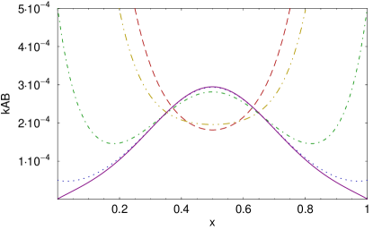
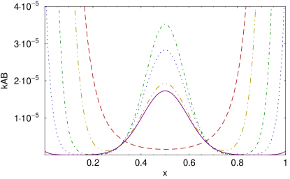
Figure 2: Stationary reaction intensity profile $kA(x)B(x)$ for $\alpha=1$ (upper panel) and for $\alpha=0.9$ (lower panel). The parameters are the same as in Fig.1, namely: $A(1)=1$ (dashed line) , $0.5$ (dash-dot-dot), $5\cdot{10^{-2}}$ (dash-dot), $5\cdot{10^{-3}}$ (dotted),and $1\cdot{10^{-4}}$ (solid line). In the diffusive case the stationary reaction intensity profile approaches a limiting form under decreasing minor source strength. For subdiffusion-reaction the height of the profile shows nonmonotonous behavior with respect to this parameter. Note the difference in vertical scales!

In the symmetric case both reaction-diffusion and reaction-subdiffusion situations correspond to a very similar behavior with maximal concentrations in the regions close to the boundaries where the system is fed by reactants. For asymmetric boundary conditions however the behaviors of the concentrations in regular diffusion and in subdiffusion differ strongly. One of the most marked differences corresponds to a strong non-monotonicity of the concentration close to the major source (side with the higher concentration of A) indicating for accumulation of A particles in the interior of the subdiffusive medium. Its counterpart on the other side of the system is a depletion zone (corresponding to the symmetric accumulation zone for B). The peak and the depletion zone are much more pronounced for smaller $\alpha$; the choice of moderate $\alpha=0.9$ was caused by our whish to show the behavior pertinent to diffusion and to subdiffusion on the same scale. It is important to note that the dependence of the height of the accumulation peak on the strength of the minor source is nonmonotonous: The reduction of the minor source strength $A(1)=B(0)$ leads first to its growth, and then to its outwards motion accompanied by decay.

Let us now turn to reaction intensities, Fig. 2. For the symmetric case the reaction takes place mostly close to the boundaries of the system. For smaller $A(1)$ the reaction zone starts to form in the middle of the system. However, also here striking differences between the reaction-diffusion and the reaction-subdiffusion cases are seen. In the reaction-diffusion case the dependence of the form of the reaction zone on $A(1)$ is weak for small $A(1)$, and there exists a clear limiting form for $A(1)=0$. This behavior is known and is used in the time-scale separation approach of Refs.Sokolov ; GalfiRatz based on the quasistatic approximation. For reaction-subdiffusion the behavior of the reaction zone with respect to its height is non-monotonous. When lowering $A(1)$, the maximum of reaction intensity first gets higher and then starts to lower; and the distribution as a whole broadens. The reason for this is quite evident. The stationary reaction zone exists only if it is fed by A- and B-reactants on the corresponding sides. Both in the diffusion and in the subdiffusion case the reaction zone is the higher and the narrower the larger is the particles’ inflow into the reaction area. This inflow is governed by the effective diffusion coefficient of the corresponding reactants, which, in the subdiffusive case, depends on the concentration of the reacting counterpart. Since the effective mobility of subdiffusing species decays in the course of time (the number of steps per unit time goes as $t^{\alpha-1}$), the effective diffusion in subdiffusion is caused by the reaction itself: it corresponds to a reaction-induced diffusion term, just as in the reactions between immobile species PostnikovSokolov ; Sander . For zero $A(1)=B(0)$ concentration the effective diffusion coefficient vanishes on the corresponding side of the system preventing the inflow of reactants from their major sources into the interior of the system. The reaction zone blurs and fades out. In this case no stationary front exists. This effect is also clearly seen when considering the time evolution of concentrations which can be done by discussing the properties of the inverse Laplace transform of Eq.(Stationary spatial structures in reaction-subdiffusion). This means that the adiabatic approximation of Refs.Sokolov ; GalfiRatz fails in subdiffusion, and the analysis of the front’s motion in this case has to be done anew.

Let us summarize our findings. We discussed the stationary form of reactants’ concentrations and of reaction zones in the $\mathrm{A}+\mathrm{B}\rightarrow 0$ reaction in a subdiffusive medium fed by reactants on its both sides. We show that the behavior of the concentration and of the reaction intensity profiles in subdiffusion differs strikingly from those in simple diffusion. The most important differences correspond to the existence of accumulation and depletion zones close to the boundaries and to non-monotonous behavior of the reaction intensity with respect to the strength of the minor source. These results have implications for the time-dependent front forms in $\mathrm{A}+\mathrm{B}\rightarrow 0$ reaction, since the adiabatic approximation used in the reaction-diffusion case would fail in the reaction-subdiffusion one.

References

- (1) I.M. Sokolov, J. Klafter and A. Blumen, Phys. Today 55 (11) 48 (2002)
- (2) J. Klafter and I.M. Sokolov, Phys. World, 18 (8) 29 (2005)
- (3) B.J. Henry and S.L. Wearne, Physica A 276 448 (2000); SIAM J. Appl. Math. 62 870 (2002); B.I. Henry, T.A.M. Langlands and S.L. Wearne, Phys. Rev. E 72 (2) 026101 (2005)
- (4) T. Kosztolowicz, K.D. Levandowska, Acta Physica Polonica B 37 1571 (2006)
- (5) S.B. Yuste, L. Acedo, K. Lindenberg, Phys. Rev. E 69 036126 (2004)
- (6) K. Seki, M. Wojcik and M. Tachiya, J. Chem. Phys. 119, 2165 (2003)
- (7) I.M.Sokolov, M.G.W. Schmidt, F. Sagués, Phys. Rev. E 73 031102 (2006)
- (8) M.G.W. Schmidt, F. Sagués, I.M.Sokolov, J. Phys. Condensed Matt. 19 065118 (2007)
- (9) A. Yadav, W. Horsthemke, Phys. Rev. E 74, 066118 (2006)
- (10) I.M. Sokolov, JETP Lett. 44 67 (1986)
- (11) L. Galfi, Z. Racz Phys. Rev. A 38 3151 (1988)
- (12) E.B. Postnikov, I.M. Sokolov, Math. Biosci. (in press) doi:10.1016/j.mbs.2006.10.004
- (13) L.M. Sander and G.V. Ghaisas, Physica A 233, 629 (1996)