Larkin-Ovchinnikov state in resonant Fermi gas
Abstract
We construct the phase diagram of a homogeneous two component Fermi gas with population imbalance under a Feshbach resonance. In particular, we study the physics and stability of the Larkin-Ovchinnikov phase. We show that this phase is stable over a much larger parameter range than what has been previously reported by other authors.
pacs:
03.75.Ss, 05.30.Fk, 34.90.+qTrapped fermi gases offer us a wonderful opportunity to study strongly interacting fermion systems expr . With Feshbach resonance, one is able to tune the effective interaction from weakly attractive for magnetic field above the resonance to strongly attractive below. This problem is also closely related to studies of quark and nuclear matter other-review
Recent attention has shifted to systems with unequal populations UNpd ; SR06 ; SR-rev ; unexpr . The latter problem is analogous to the physics of a superconductor under the influence of an external Zeeman field, which provides a chemical potential difference between the two species and . In the weak-coupling limit, it was shown by Sarma Sarma that the uniform state with population imbalance is unstable at zero temperature. By comparing the free energy of the normal state and the completely paired superconducting state, he concluded that, as the magnetic field is increased, there is a first order phase transition from the equal-population superconducting state (with gap ) to the normal state at . This implies that a system with given unequal numbers of the two spin species will either phase separate(with ), or be in the normal state (with ), depending on the imbalance. However, later, Fulde-Ferrell FF and Larkin-Ovchinnikov LO showed that there are better alternatives. Fulde and Ferrell (FF) considered a state with order parameter , that is, pairs with finite momentum. The order parameter has a spatially varying phase with however the magnitude still constant in space. They showed that in certain parameter space this state has lower free energy than the states considered by Sarma. Larkin and Ovchinnikov (LO), however demonstrated that, at least in the small order parameter limit, states with certain choices of sinusoidal variations of order parameter (such as etc) are more energetically favorable than the FF state. Notice that in the LO state, the magnitude of the order parameter is no longer a constant in space. With decreasing magnetic field and hence decreasing population difference , many authors showed that the LO state evolves into a state with a set of domain walls. This has been demonstrated for one 1D , two Burkhardt , as well as in three Nagai dimensions and also for a d-wave superconductor Vorontsov . In the small population imbalance limit, the order parameter has a constant magnitude almost everywhere in space (with value identical to the state with no population difference), except near the domain walls. The phase of the order parameter changes by when these walls are crossed, and these are also the locations where the magnetization concentrates. This local magnetization arises from the occupation of bound states, available due to the presence of the domain walls. The physics of these domain walls is closely related to the -junctions in SFS (S=superconductor, F=ferromagnet) junctions Buzdin , where for suitable parameters it is energetically favorable for the two superconductors to acquire a phase difference .
Indeed, in three-dimensions, in the zero temperature and weak-coupling limit, Matsuo et al Nagai demonstrated that the energy of the domain walls becomes negative for above where is the zero temperature gap for the completely-paired superfluid of equal populations. This is less than the phase separation field (where the free energy of the normal and the completely-paired superfluid states are equal). Hence the LO state must be more stable than both the uniform superfluid and the normal state (at least) for . For slightly above , the domain walls are far apart. The system resembles the uniform paired state except for the occasional domain walls. This state thus allows for the possibility of arbitrarily small population difference between the two species. This problem is quite analogous to the lower critical field in type II superconductors, where the vortex energy becomes negative and vortices begin to penetrate the superconductor for slightly above . For increasing , more and more domain walls are formed, the order parameter becomes more sinusoidal like and the state evolves smoothly to the picture given by LO LO .
For the resonant Fermi gas, it has been recognized that at intermediate coupling strengths, the uniform state with population imbalance must be unstable UNpd ; SR06 . Indeed this has also been demonstrated also by experiments unexpr . However, the investigation into the actual phase diagram, that is, the question as to which phase appears where instead of the unstable uniform state, even for the case without a trap, cannot be regarded as complete, especially regarding the stability of the FFLO states. Many papers Parish07 ; Gu06 examined only phase separation, whereas some SR06 ; SR-rev ; Hu06 ; He06 ; YanHe07 considered in addition only the FF state with . However, none of these works actually investigated the LO states. They conclude that the FF state exists only in a very narrow region next to the normal state in the weak-coupling regime, and deduce then that phase-separation occurs throughout the rest of the entire region where the uniform phase is unstable. In particular, they conclude that, for small population differences, phase separation occurs unless the dimensionless coupling constant . However, as seen already in the above paragraph, this is simply an artifact of the FF state, which cannot smoothly go into the completely paired equal population state Takada . We expect that at least, in the weak-coupling limit, the state should be LO for any population imbalance below that of the normal state.
In this work, we shall investigate the stability of the LO state for arbitrary strength of the attractive interaction between the two species, thus generalizing previous works such as Burkhardt ; Nagai beyond the BCS limit. We shall concentrate in particular on the small limit. More specifically, we compare the critical chemical potential difference at which the domain wall energy becomes negative, to the critical field for phase separation where the free energy of the normal phase becomes equal to that of the completely paired equal population superfluid phase. We find that for , . Therefore we conclude that, for small , the LO state is more stable than the phase separated state for . By combining with previous results UNpd ; SR-rev ; UN-reply (and with some reasonable extrapolations), we sketch the appropriate phase diagram for our system.
The mean-field Hamiltonian of our system can be written as
| (1) |
where , for the two species, their corresponding field operators, a position dependent order parameter and the coupling constant. For convenience below we shall also write and .
This Hamiltonian can be diagonalized by the Bogoliubov transformation for a general inhomogeneous system deGennes :
| (8) |
where , are annihilation operators for quasiparticles with spin and of the state labelled by a set of quantum numbers . , obeys and the Bogoliubov-deGennes (B-dG) equation
| (15) |
Substituting eq (8) into eq (1) and using eq (15) to eliminate the derivatives and ’s, we obtain the ground state free energy
| (16) |
The last term arises from the occupation of states with . Here is the Fermi function, the volume, and we have eliminated the interaction constant in favor of the scattering length via the relation where is the energy of the state in the normal phase. (Strictly speaking we should label the quantum states in the normal phase by another set of quantum numbers , but we shall not make such a distinction for simplicity in notations. See further below.) In eq (16), should be viewed as a variational parameter with respect to which has to be minimized.
We are interested in the domain wall energy for given , and . We evaluate this by calculating the energy difference between a state with a single planar domain wall and the uniform completely paired superfluid state. The latter is easy, since it is independent of and the B-dG equation (15) can be solved by Fourier transform. We obtained, for wavevector , the familiar quasiparticle energies (where ) and hence the bulk free energy . Minimizing with respect to gives the usual BCS gap equation . We can also compute the corresponding density via and the corresponding Fermi wavevector and express in the dimensionless combination . These results are identical with those in Engelbrecht . We had also used instead of a domain wall in the procedure described below and verified numerically that we indeed obtained the same free energy density for the uniform state. [Equating this free energy to that of the normal state at the same and , we obtained the phase separation field discussed.]
Next we evaluate the free energy of a planar domain wall. For this, we put our system in a box of dimensions , , . We assume that the order parameter varies only along the direction and thus Fourier transform the and coordinates. Calling the resulting wavevector , we rewrite as
| (21) |
where is the component of in the x-y plane, and is now a quantum number for the dependences. are dimensionless quantities obeying . Eq (15) becomes
| (28) |
where . The energies and the wavefunctions , depend on only through its magnitude . The free energy can then be written as
| (29) |
In this equation, we arrange the quasiparticle states for both the superfluid and the normal states as increasing function of the counting number . We solve eq (28) by discretizing the coordinate. After the energies and the function are calculated, we put it in eq (29) and calculate the free energy. For , we limit ourselves to the one-parameter ansatz
| (30) |
with as the variational parameter and . (Thus the width of the domain wall is given by .) Here is the bulk order parameter for the given and at , as the order parameter should approach this value far away from the domain wall. Our eq (30) is motivated by earlier investigations Burkhardt ; Nagai , where their numerical results can be well fitted by a function of the form (30). (Since we are employing periodic boundary conditions in , this ansatz actually introduces a sharp () domain wall also at . However, this can be taken care of easily by removing the contributions due to this extra domain wall.)
We shall then input the ansatz eq (30) into eq (28) to solve for . Our analysis of the free energy eq (29) is simplified by the following observations. At , since all quasiparticle energies are positive, and the free energy is given simply by the integral in eq (29). The free energy at finite of a given is related to that of at the same by simply adding the negative term due to the occupation of the quasiparticle states.
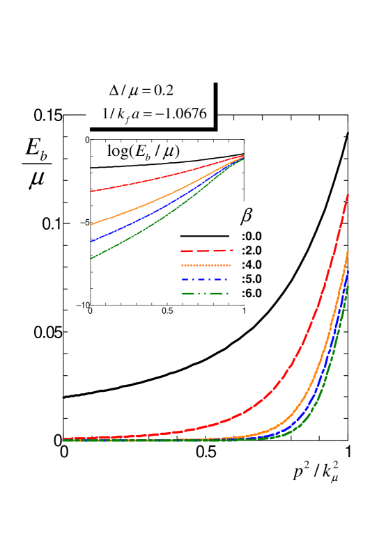
An example for our results for , and are discussed below. The bound state energies are illustrated in Fig 1. We see that in general we have states below the continuum ( for , for . It is the bound states that are essential: as we shall see, the relevant values of are below the gap edges). The results were checked against the analytical ones in the Appendix. The bound state energy for a given decreases with the width of the domain walls, as one expects. The significance of this would be discussed again below.
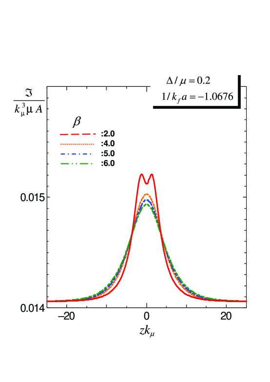
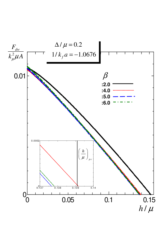
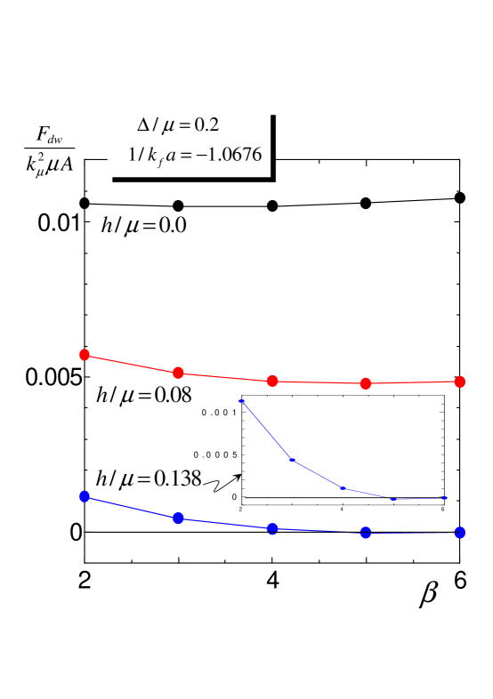
The integrand of the first term in eq (29) is plotted in Fig 2. (The double hump structure for small () is due to the fact that as : see eq (29)). As expected, the integrand decreases to a constant corresponding to the free energy density in the bulk for distances sufficiently far away from the domain wall. We can then evaluate the domain wall energy at by simply integrating this excess contribution over . At , is minimum at . is positive for all ’s, as expected since the uniform state should have a lower energy than a domain wall. For finite , the free energies are evaluated by adding the negative term from bound state occupation as discussed above. The results are depicted in Fig 3. The free energy decreases due to the occupation of the bound states. Since the bound state energies are smaller for larger , the wall energy decreases faster for larger , shifting the for minimum wall energy to larger values with increasing (see Fig 4). The domain wall energy becomes negative at sufficiently large for all ’s. The important question is whether it will become negative for some at a value of which is less than that for phase separation. For the parameters under discussion, the domain wall energy first becomes negative for at , which is less than the phase separation value . We thus conclude that for , when is infinitesimally small, the system is in the LO state but not the phase separated state.
At this point, it is of interest to compare our results more quantitatively with those in Nagai , who has assumed the quasiclassical limit in their calculations at the outset. They obtained the critical value for the sign change of the domain wall energy at (using ). Our is close to their value if we simply rewrite their result as and substitute . Also, their Fig 1 indicates a domain wall width near the critical field to be roughly given by where is the Fermi velocity. Rewriting this expression as and simply subsituting the values of etc we again find very good agreement. Thus, even though we did not assume the quasiclassical limit at the outset, for our results can be understood from the quasiclassical limit calculations of Nagai with extrapolations.
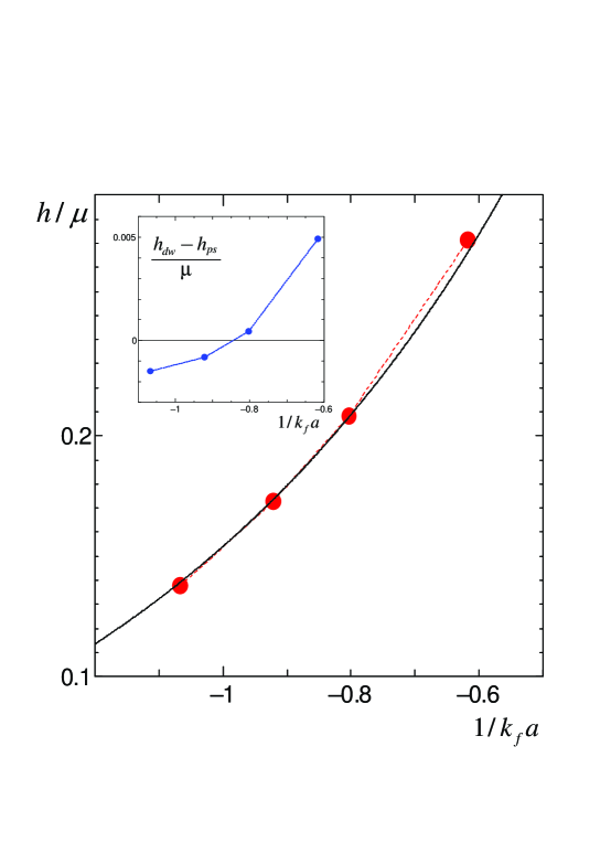
For increasing , both and increase (and the for the optimal domain wall decreases). However, increases faster than , and eventually no longer holds. The situation is shown in Fig 5. If , then the formation of domain wall is no longer favorable since phase separation already occurs at slightly above . We conclude then, for , the transition from the LO state to the phase separation state occurs at . This point is indicated by the point A in Fig 6.
After locating this transition point for , we now attempt to construct a phase diagram for general by combining the present results with previous ones in the literature. For and sufficiently negative , the system is in the normal state UNpd ; SR-rev . We consider in turn the transition lines between this normal state and the LO and phase separated states. Assuming that the transition to the LO state is second order LO (c.f. below), the transition line between the normal and LO state can be found by solving the Cooper problem at finite wavevector :
| (31) |
The transition line is determined by finding the optimal corresponding to the weakest attractive interaction, i.e., the most negative . We note here that, since eq (31) is obtained by linearizing in the order parameter, the same equation determines the second order transition line into the FF state LO . Our result can be turned into a line in our phase diagram (an equation of versus ) by using , with and . This gives the long-dashed line in Fig 6. Our numerical results (see also UN-reply ) agree well with SR-rev . It should however be remarked that the transition from the normal state to the LO state has also claimed to be first order Mora05 at very low temperatures in three-dimensions. However, the difference between the actual transition line and the second order line is very small Mora05 , and we ignore this difference here.
For the transition line between the normal state and phase separation, we equate Sarma the free energy of the completely paired superfluid state to that of the normal state: . This again yields a line as a function of and hence , shown as the solid line in fig 6. Our numerical result (see also UN-reply ) is also in good agreement with SR-rev . The two transition lines intersect at the point labelled by X at . Therefore the transition is to the LO (phase separation) state if is less (larger) than this value. Interpolating between points A and X, we thus conclude that the system is in the LO state for the shaded region to the right of the line XA, whereas phase separation occurs for the shaded region to the left of this line. The transition lines between this phase-separated state and the homogeneous superfluid (Bose-Fermi mixture) phase for positive have already been discussed elsewhere in the literature ( SR-rev ; Parish07 ; Gu06 , see also other references in UN-reply ), and we would not repeat the details here.
In conclusion, we studied the stability of the LO state in a homogeneous system, in particular in the limit of small population imbalance, by calculating the domain wall energies. Our investigation here is analogous to the determination of the lower critical field of the vortex phase of a type II superconductor. The determination of the detailed structures of the LO state, such as the question of the lattice structure of the domain walls (c.f. e.g. Mora05 , analogous to the vortex lattice structure in type II superconductors), as well as the phase diagram in the presence of a trap (studied already partially in LOtrap ), are left for the future.
We thank C.-H. Cheng, C.-H. Pao and S.-T. Wu for their help in obtaining the transition lines from the normal state. This research was supported by the National Science Council of Taiwan under grant number NSC95-2112-M-054-MY3.
Appendix – Bound states
Due to the important role played by the bound states in the LO state, we give the analytic results for a sharp domain wall where (corresponding to ). It should be noted that, even though is a constant throughout in space, bound states still exist due to the sudden change in phase factor of the order parameter from to at . As already seen from eq (28), the bound state energy is a function of and only through the combination . The B-dG equation (28) can be solved easily in this case since is piecewise constant. We require that the functions , as well as their derivatives be continuous at . The calculation is similar to solving the Schrödinger equation in piecewise constant potentials. It is straightforward and we simply state the results. It is convenient to divide them into two regions:
(i) . In this case states are bound when . We find that there is only one bound state (thus correspondingly one bound state for each ), with energy given by
| (32) |
where . We note here that the quasiclassical limit corresponds to hence . In this limit, one can approximate the B-dG equation by the Andreev equation Andreev64 and the bound state energy vanishes (irrespective of the detailed positional dependence of so long as there is a phase change: see e.g Lofwander and also Atiyah ). For small , we have . (c.f. the mini-gap for bound states near the vortex core deGennes ). With increasing or equivalently decreasing , increases. For , .
(ii) . In this case the continnuum starts at . Again we find only one bound state, with
| (33) |
where . For (), (c.f. case (i) above). For decreasing (decreasing ), increases. reaches at . For , approaches the continuum from below. It is remarkable that bound state exists even for . We note that in this regime we have always . A similar situation occurs also for the bound states at a vortex Sensarma for general coupling strength .
References
- (1) C. A. Regal, M. Greiner, and D.S. Jin, Phys. Rev. Lett. 92, 040403 (2004); T. Bourdel et al, ibid. 93, 050401 (2004); C. Chin et al., Science 305, 1128 (2004); J. Kinast et al., ibid. 307, 1296 (2005); M. W. Zwierlein et al, Nature (London) 435, 1047 (2005); and references therein.
- (2) R. Casalbuoni and G. Nardulli, Rev. Mod. Phys. 76, 263 (2004)
- (3) C.-H. Pao, S.-T. Wu and S.-K. Yip, Phys. Rev. B 73, 132506 (2006); ibid, 74, 189901(E) (2006).
- (4) D. E. Sheehy and L. Radzihovsky, Phys. Rev. Lett. 96, 060401 (2006)
- (5) D. E. Sheehy and L. Radzihovsky, cond-mat/0607803
- (6) M. W. Zwierlein, Andre Schirotzek, Christian H. Schunck, and Wolfgang Ketterle, Science 311, 492 (2006); G. B. Partridge, Wenhui Li, Ramsey I. Kamar, Yean-an Liao, and Randall G. Hulet, ibid, 311, 503 (2006); M.W. Zwierlein, C.H. Schunck, A. Schirotzek, and W. Ketterle, Nature 442, 54 (2006); Y. Shin, M. W. Zwierlein, C. H. Schunck, A. Schirotzek, and W. Ketterle, Phys. Rev. Lett. 97, 030401 (2006); G. B. Partridge, Wenhui Li, Yean-an Liao, Randall G. Hulet, M. Haque and H. T. C. Stoof, ibid, 97, 190407 (2006).
- (7) G. Sarma, J. Phys. Chem. Solids, 24, 1029 (1963)
- (8) P. Fulde and R. A. Ferrell, Phys. Rev. 135, A550 (1964)
- (9) A. I. Larkin and Yu. N. Ovchinnikov, Zh. Éksp. Teor. Fiz. 47, 1136 (1964) [Sov. Phys. JETP 20, 762 (1965)].
- (10) K. Machida and H. Nakanishi, Phys. Rev. B 30, 122 (1984); A. Buzdin and S. Polonski, Sov. Phys. JETP 66, 422 (1987). These two papers assumed mean-field theory applies. See further K. Yang, Phys. Rev. B 63, 140511(R) (2001).
- (11) H. Burkhardt and D. Rainer, Ann. Phys. (Leipzig) 3, 181 (1994)
- (12) S. Matsuo, S. Higashitani, Y. Nagato and K. Nagai, J. Phys. Soc. Jpn. 67, 280 (1998)
- (13) A. B. Vorontsov, J. A. Sauls and M. J. Graf, Phys. Rev. B 72, 184501 (2005)
- (14) A. I. Buzdin, Rev. Mod. Phys. 77, 935 (2005)
- (15) M. M. Parish, F. M. Marchetti, A. Lamacraft and B. D. Simons, Nature Physics, 3, issue 2, 124 (2007)
- (16) Z.-C. Gu, G. Warner and F. Zhou, cond-mat/0603190
- (17) H. Hu and X.-J. Liu, Phys. Rev. A 73, 051603(R) (2006)
- (18) Lianye He, M. Jin and P. Zhuang, Phys. Rev. B 73, 214527 (2006)
- (19) Yan He, C.-C. Chien, Q. Chen and K. Levin, Phys. Rev. A 75, 021602(R) (2007)
- (20) S. Takada and T. Izuyama, Prog. Theor. Phys. 41, 635 (1969)
- (21) P. G. deGennes, Superconductivity of Metals and Alloys, 1989, Addision-Wesley.
- (22) J. R. Engelbrecht, M. Randeria and C. A. R. Sa de Melo, Phys. Rev. B, 55, 15153 (1997)
- (23) C.-H. Pao, S.-T. Wu and S.-K. Yip, cond-mat/0608501
- (24) C. Mora and R. Combescot, Phys. Rev. B 71, 214504 (2005); see also H. Shimihara, J. Phys. Soc. Jpn, 67, 736 (1998)
- (25) J. Kinnunen, L. M. Jensen and P. Törma, Phys. Rev. Lett. 96, 110403 (2006). K. Machida, T. Mizushima and M. Ichioka, ibid, 97, 120407 (2006)
- (26) A. F. Andreev, Zh. Eksp. Teor. Fiz. 46, 1823 (1964) [Sov. Phys. JETP 19, 1228 (1964)]
- (27) T. Löfwander, V. S. Shumeiko and G. Wendin, Supercond. Sci. Technol. 14, R53 (2001)
- (28) M. Atiyah, V. Patodi and I. Singer, Cambridge Philos. Soc. 77, 43 (1975)
- (29) R. Sensarma, M. Randeria and T.-L. Ho, Phys. Rev. Lett. 96, 090403 (2006)