Tunable quantum dots in bilayer graphene

Abstract

We demonstrate theoretically that quantum dots in bilayers of graphene can be realized. A position-dependent doping breaks the equivalence between the upper and lower layer and lifts the degeneracy of the positive and negative momentum states of the dot. Numerical results show the simultaneous presence of electron and hole confined states for certain doping profiles and a remarkable angular momentum dependence of the quantum dot spectrum which is in sharp contrast with that for conventional semiconductor quantum dots. We predict that the optical spectrum will consist of a series of non-equidistant peaks.

Two-dimensional (2D) carbon crystals, such as single-layer and bilayer graphene, have been the subject of increasing interest due to the unusual mechanical and electronic properties, which may lead to their use in novel nanoelectronic devices. The relativistic-like properties of carriers in single-layer graphene zheng ; novo3 ; novo4 ; shara ; zhang result from the gapless and approximately linear electron spectrum near the Fermi energy at two inequivalent points of the Brillouin zone. The charge carriers in these structures are described as massless relativistic fermions and are governed by the Dirac equation. In contrast, for a symmetric graphene bilayer the spectrum is parabolic at the vicinity of the $K$ points.

Among the unusual properties of single-layer graphene is the perfect forward transmission across potential barriers, known as Klein tunneling klein ; Katsnelson , which is related to the absence of a gap in the carrier spectrum. This effect prevents the electrostatic confinement of charged particles and thus the realization of quantum dots. Recently, alternative strategies have been proposed to confine charged particles by using thin single-layer graphene strips Peres ; Efetov or non-uniform magnetic fields Egger . Here we propose a novel approach by considering a bilayer graphene, in which a charge imbalance between the layers gives rise to a gap in the spectrum, that can be used to create potential barriers Falko ; Geim . Such bilayers of graphene can be obtained, e.g., from a graphite crystal by micromechanical cleavage novo2 . A recent report described the synthesis of bilayer graphene sheets by graphitization of silicon carbide (SiC) surfaces in which the equivalence of the two graphene layers is broken by their interaction with the SiC substrate as well as by doping one of them with potassium atoms Ohta .

These recent experimental progresses raise the possibility of introducing a position-dependent modification of the spectrum at the Dirac point by changing the potassium density at different regions of the bilayer graphene sheet or by using microstructured gates. In this letter we propose a position-dependent potassium doping to manipulate the band structure of bilayer graphene in order to create nanometer-scale quantum structures such as quantum dots. Semiconductor quantum dots have been intensively investigated both theoretically and experimentally. Up to now, only quantum dots on graphiteBunch have been obtained, with sample thicknesses of several nanometers, i.e., of the order of $10$ stacked graphene layers. Theoretical calculations show that the properties of a bilayer graphene can be significantly distinct from such multilayer systems Bart . In the present work we demonstrate that the electronic states of such quantum dots can differ significantly from the usual semiconductor-based dots.

The crystal structure of an undoped bilayer of graphene is that of two honeycomb sheets of covalent-bond carbon atoms coupled by weak Van der Waals forces. To each carbon atom corresponds a valence electron and the structure can be described in terms of four sublattices, labelled A, B (upper layer) and A^′, B^′ (lower layer). Considering only nearest-neighbor hoping, the Hamiltonian of the system in the vicinity of the ${\mathbf{K}}$ point is given, in the continuum approximation, by Snyman

$$\mathcal{H}=\mathcal{H}_{0}+(\Delta U/2)\tau_{z},$$ (1)

with

$$\mathcal{H}_{0}=\begin{pmatrix}U_{0}&\pi&t&0\\ \pi^{\dagger}&U_{0}&0&0\\ t&0&U_{0}&\pi^{\dagger}\\ 0&0&\pi&U_{0}\end{pmatrix},$$ (2)

where $t\approx 400$ meV is the interlayer coupling term, $\pi=v_{F}(p_{x}+ip_{y})$, $\hat{\mathbf{p}}=(p_{x},p_{y})$ is the 2D momentum operator, $v_{F}\approx 1\times 10^{6}$ m/s, $U_{0}=(U_{1}+U_{2})/2$, $\Delta U=U_{1}-U_{2}$ and $U_{1}$, $U_{2}$ are the potentials at the two layers, which reflect the influence of doping on one of them and/or the interaction with an external electric field, i.e., the gating. The operator $\tau_{z}$ assigns a positive (negative) sign to the upper (lower) layer labels and is defined as

Figure 1: Lower panel: schematics of the quantum dot layout, showing the doped graphene layer (brown) and the quantum dot region (light brown). Upper panel: the induced parabolic potential and the energy levels of the confined states.

$$\tau_{z}=\begin{pmatrix}\mathbf{I}&0\\ 0&-\mathbf{I}\end{pmatrix},$$ (3)

with $\mathbf{I}$ denoting the $2\times 2$ identity matrix. The eigenstates of Eq. (1) are four-component spinors $\Psi=[\psi_{A}\,,\,\psi_{B}\,,\,\psi_{B^{\prime}}\,,\,\psi_{A^{\prime}}]^{T}$, where $\psi_{A,B}$ ($\psi_{A^{\prime},B^{\prime}}$) are the envelope functions associated with the probability amplitudes at the respective sublattice sites of the upper (lower) graphene sheet. One can also define an inversion operator $\mathbf{X}$ as

$$\mathbf{X}=\begin{pmatrix}0&\mathbf{I}\\ \mathbf{I}&0\end{pmatrix},$$ (4)

which acts on $\Psi$ by changing $A$ to $B^{\prime}$ and $B$ to $A^{\prime}$. It is seen that for finite $\Delta U$, the Hamiltonian (1) does not commute with $\mathbf{X}$; this results from the lack of inversion symmetry in the system.

For constant potentials $U_{1}$ and $U_{2}$, the single-particle spectrum consists of four bands that correspond to the solutions of the equation $[s_{F}^{2}-(E-U_{1})^{2}][s_{F}^{2}-(E-U_{2})^{2}]-t^{2}(E-U_{1})(E-U_{2})=0$ with $s_{F}=\hbar v_{F}k$, given by

$$E^{+}_{\pm}(k)=U_{0}+(1/2)\big{[}(t\pm\Gamma)^{2}+\Omega\big{]}^{1/2},$$ (5)

(6)

$$E^{-}_{\pm}(k)=U_{0}-(1/2)\big{[}(t\pm\Gamma)^{2}+\Omega\big{]}^{1/2},$$ (7)

where $\Gamma=\big{[}t^{2}+4s_{F}^{2}+4(s_{F}^{2}/t^{2})\Delta U^{2}\big{]}^{1/2}$ and $\Omega=\big{[}1-4s_{F}^{2}/t^{2}\big{]}\Delta U^{2}$. Note that for $k=0$ the spectrum shows a gap at $k=0$ of size $E^{+}_{-}(0)-E^{-}_{-}(0)=|\Delta U|$ and the system becomes a narrow-gap semiconductor. Figure 2 shows the spectra for $U_{1}=U_{2}=0$ (dashed red curve), $U_{1}=200$ meV and $U_{2}=0$ (solid black), and $U_{1}=-U_{2}=100$ meV (dot-dashed blue curve). The existence of such a gap allows the creation of nanostructures based on a position-dependent doping, which in turn can create a position-dependent potential difference between the upper and lower layers of the structure Castro2 . Different potentials $U_{1}$ and $U_{2}$ can be created on defect-free graphene by controlling the deposition of potassium atoms on the upper layer or by applying gate electrodes Geim .

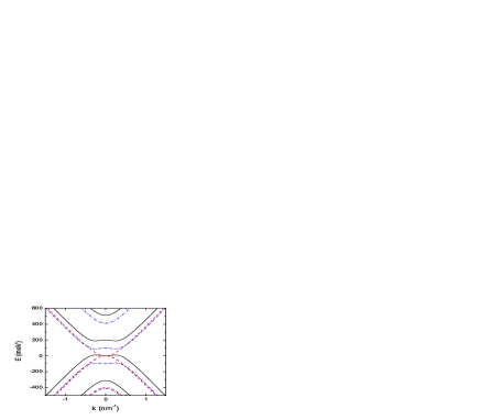
Figure 2: Spectrum of a graphene bilayer with $U_{1}=U_{2}=0$ (dashed curve), $U_{1}=200$ meV and $U_{2}=0$ (solid curve), and $U_{1}=-U_{2}=100$ meV (dot-dashed curve).

The next step is to use a non-uniform doping, or microstructured gate electrodes, that will lead to a position-dependent potential difference between the layers. In the experimental system studied in Ref. Ohta, there was a potential difference $\Delta U$ between the graphene layers even in the absence of doping, due to their interaction with the SiC substrate. In that case the potentials were equalized when the number of doping electrons per unit cell was $\gamma_{0}=0.0125$. For the sake of simplicity we assume a constant interlayer hopping term $t$ though in reality $t$ may depend on the doping level. In the present case a small change of the value of $t$ will not affect significantly the results for low energies. The experimental results show that $\Delta U$ scales approximately linearly with doping over a wide range of potassium concentration levels.

A position-dependent, circular-symmetric profile $\gamma({\mathbf{r}})=\gamma(\rho)$ gives rise to a 2D circular-symmetric quantum dot of radius $R$ on a bilayer graphene, shown schematically in Fig. 1, with the doping level ranging from $\gamma_{0}$ at $\rho=0$ to a maximum value $\gamma_{M}$ for $\rho>R$. In that case the four-component spinors $\Psi$ are given byVincenzo

$$\Psi(\rho,\theta)=\begin{pmatrix}\phi_{A}(\rho)e^{im\theta}\\ \ \\ i\phi_{B}(\rho)e^{i(m-1)\theta}\\ \ \\ \phi_{B^{\prime}}(\rho)e^{im\theta}\\ \ \\ i\phi_{A^{\prime}}(\rho)e^{i(m+1)\theta}\end{pmatrix},$$ (8)

where $m$ is an integer. $\Psi$ are eigenstates of the operator

$$J_{z}=L_{z}+\frac{\hbar}{2}\tau_{z}-\frac{\hbar}{2}\begin{pmatrix}\sigma_{z}&0\\ 0&-\sigma_{z}\end{pmatrix}$$ (9)

with eigenvalue $m$; $L_{z}$ is the angular momentum operator and $\sigma_{z}$ the Pauli matrix. This represents the total angular momentum of the carrier and the layer index operator, which is associated with the behavior of the system under inversion.

The potential difference between the layers is $\Delta U=U(\rho)$ and subsequently the equations for the radial part of the spinor functions are

$$\big{[}d/d\zeta+m/\zeta\big{]}\phi_{A}=\Omega_{1}\phi_{B},$$ (10)

(11)

$$\big{[}d/d\zeta-(m-1)/\zeta\big{]}\phi_{B}=-\Omega_{1}\phi_{A}+t^{\prime}\phi_{B^{\prime}},$$ (12)

(13)

$$\big{[}d/d\zeta+(m+1)/\zeta\big{]}\phi_{A^{\prime}}=-\Omega_{2}\phi_{B^{\prime}}+t^{\prime}\phi_{A},$$ (14)

(15)

$$\big{[}d/d\zeta-m/\zeta\big{]}\phi_{B^{\prime}}=\Omega_{2}\phi_{A^{\prime}},$$ (16)

where $\zeta=\rho/R$, $\Omega_{1,2}=\epsilon-u_{1,2},$ $u_{1,2}=U_{1,2}R/\hbar v_{F}$, $\epsilon=ER/\hbar v_{F}$, and $t^{\prime}=tR/\hbar v_{F}$. The $m\pm 1$ that appear in Eqs. (10) and (11) are a direct consequence of the presence of a geometric phase in the system (i.e. a full rotation of the system introduces a phase difference of $2\pi$ between the sublattice sites $A^{\prime}$ and B). In addition, the large magnitude of the layer coupling term $t^{\prime}$, in comparison with the other energy terms, implies that the $\phi_{B}$ and $\phi_{A^{\prime}}$ must have significantly higher amplitudes than $\phi_{A}$ and $\phi_{B^{\prime}}$. These two facts have important consequences for the energy spectrum and the shape of the resulting probability density functions, as we show below.

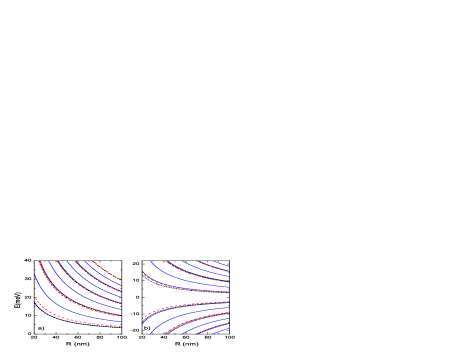
Figure 3: Lowest energy states of a graphene bilayer quantum dot for $m=0$ (blue solid line), $m=1$ (black dotted line) and $m=-1$ (red dashed), for (a) $U_{M}=50$ meV and $U_{2}=0$ and (b) $U_{1}=-U_{2}$ and $U_{M}=100$ meV.

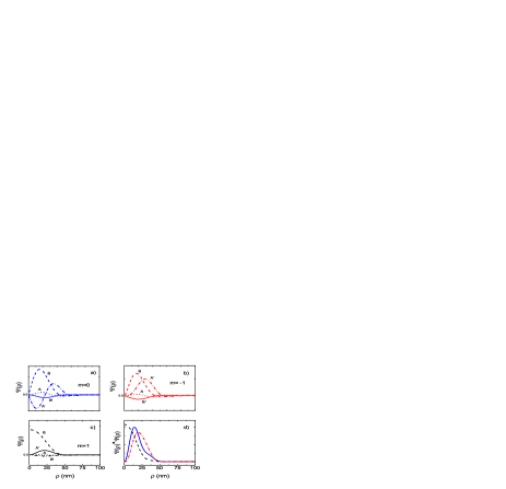
Figure 4: Panels (a)-(c): Radial dependence of the spinor functions for a parabolic quantum dot on a doped bilayer graphene for $m=0$, and $m=\pm 1$. Panel (d): probability density for each case. The parameters are $R=50$ nm, $U_{1}=50$ meV and $U_{2}=0$.

For the numerical calculations we took a truncated parabolic profile $\Delta U=U_{M}\zeta^{2}$, for $\zeta<1$ and $\Delta U=U_{M}$ otherwise. The energies of the lowest energy bound states are shown in Fig. 3 as function of the radius of the dot. Figure 3(a) shows the case $U_{2}=0$, $U_{M}=50$ meV and Fig. 3(b) the case $U_{1}=-U_{2}$, $U_{M}=100$ meV. In both cases the spectrum is proportional to the inverse of the dot radius and each set of energy levels are approximately equally spaced for fixed $m$. The results correspond to the lowest energy levels for $m=0$ (blue solid lines), $m=-1$ (red dashed), and $m=+1$ (black dotted lines). An important difference between (a) and (b) is the absence of hole bound states in (a), since there is an overlap between the hole band states in the well and the corresponding band in the barriers, whereas in (b) both electron and hole confined states are present. We found the remarkable result that the ground state is almost degenerate for $m=0$ and $m=\pm 1$ in both cases (a) and (b). This turns out to be a consequence of the geometric phase which shifts the angular momentum labels in Eqs. (10) and (11). In comparison to the results for semiconductor quantum dots we find that in a graphene bilayer there is a peculiar energy shift between states with positive and negative angular momentum even in the absence of an external magnetic field. This is a consequence of the lack of inversion symmetry in the system when $U_{1}\neq U_{2}$. The shift is larger for the low-lying states, with the $+m$ and $-m$ states becoming nearly degenerate as the energy increases. A similar, albeit weaker, shift is found for $|m|>1$.

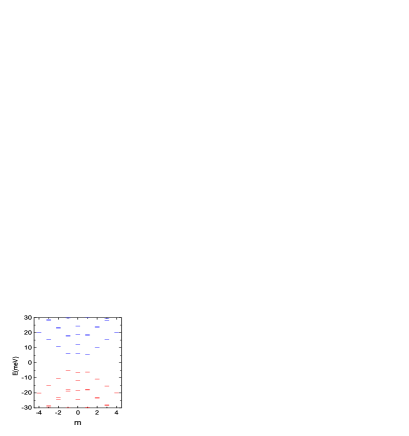
Figure 5: Energy spectrum as a function of angular momentum label $m$ for $R=50$ nm, and $U_{1}=-U_{2}=50$ meV.

The radial part of the spinor functions for some lowest energy states is shown in Fig. 4 for $m=0$ (a), $m=-1$ (b), and $m=1$ (c). Panel (d) shows the probability density ($\Psi^{*}\Psi$) for $m=0$ (solid black curve), $m=-1$ (blue dot-dashed curve) and $m=1$ (red dashed curve). All results were obtained with $U_{1}=50$ meV, $R=50$ nm, and $U_{2}=0$. In contrast to a semiconductor quantum dot, the present results show that the probability density for $m=0$ has a maximum at $\rho\neq 0$. This is due to the fact that, for $m=0$, the high-amplitude spinor components (i.e. $\phi_{B}$ and $\phi_{A^{\prime}}$) vanish at the origin. In contrast, for $m=1$, which is here the ground state, one of the high-amplitude spinor functions is allowed to assume non-zero values at the origin. In other words, for $m=1$, an electron encircling the dot adds an angular momentum phase of $2\pi$ which can be cancelled by a Berry’s phase of $-2\pi$. The shift between the low-lying energy levels of positive and negative momentum labels is evident in Fig. 5, which shows results for a quantum dot with $U_{2}=-U_{1}$ and $R=50$ nm. The results is this case show that the energy eigenvalues are related by $E(m)=-E(-m)$. This is consistent with Eqs. (9)-(12) and in sharp contrast with the relation $E(m)=E(-m)$ satisfied in a usual quantum dot with parabolic confinement. A similar behavior was observed for other potential profiles, such as the square quantum dot and the tangent hyperbolic potential.

Figure 6 shows the oscillator strengths for the allowed transitions $(m,n)\rightarrow(m\pm 1,n^{\prime})$ between the three lowest energy states (i.e. $m=0$ and $\pm 1$) within the energy window of $0<\Delta E<9$ meV, in a quantum dot of radius $R=50$ nm with $U_{1}=-U_{2}=50$ meV. Since the energy levels for different $m$ are not equally spaced, the results show the matrix elements at several values of $\Delta E$. This differs considerably from the case of the parabolic quantum dots in semiconductors, in which the transitions occur at a single energy. These transitions can be probed by means of far infrared spectroscopy measurements.

Figure 6: Oscillator strengths for transitions between the lowest energy levels $(m,n)$ in quantum dot of radius $R=50$ nm with $U_{1}=-U_{2}=50$ meV.

In summary, we proposed a novel approach to electrically confine charge carriers in 2D quantum dots in bilayer graphene. The quantum dots are created through a position-dependent doping which breaks the equivalence between the upper and lower layers. A further tuning of the quantum dot can be realized through the use of gates. The numerical results show that the degeneracy of the positive and negative momentum states of the dot is lifted even in the absence of an external magnetic field. This result differs fundamentally from that for conventional semiconductor quantum dots and arises due to the lack of inversion symmetry caused by the doping. The system can be realized experimentally by a suitable choice of doping levels or with the application of electric fields.

Acknowledgements This work was supported by the Brazilian Council for Research (CNPq), BOF-UA, the Flemish Science Foundation (FWO-Vl), the Belgian Science Policy (IUAP) and the Canadian NSERC Grant No. OGP0121756.

References

- (1) Y. Zheng and T. Ando, Phys. Rev. B 65, 245420 (2002).
- (2) K. S. Novoselov, A. K. Geim, S. V. Morozov, D. Jiang, Y. Zhang, S. V. Dubonos, I. V. Grigorieva, and A. A. Firsov, Science, 306, 666 (2004).
- (3) K. S. Novoselov, A. K. Geim, S. V. Morozov, D. Jiang, M. I. Katsnelson, I. V. Grigorieva, S. V. Dubonos, and A. A. Firsov, Nature (London) 438, 197 (2005).
- (4) Y. Zhang, Y. W. Tan, H. L. Stormer, and P. Kim, Nature (London) 438, 201 (2005).
- (5) V. P. Gusynin and S. G. Sharapov, Phys. Rev. Lett. 95, 146801 (2005).
- (6) O. Klein, Z. Phys. 53, 157 (1929).
- (7) M. I. Katsnelson, K. S. Novoselov, and A. K. Geim Nature Physics 2, 9, 620 (2006).
- (8) N. M. R. Peres, A. H. Castro Neto, and F. Guinea, Phys. Rev. B 73, 241403 (2006).
- (9) P. G. Silvestrov and K. B. Efetov, cond-mat/0606620
- (10) A. De Martino, L. Dell’Anna, and R. Egger, cond-mat/0610290
- (11) E. McCann and V. I. Fal’ko, Phys. Rev. Lett. 96, 086805 (2006).
- (12) E. V. Castro, K. S. Novoselov, S. V. Morozov, N. M. R. Peres, J. M. B. Lopes dos Santos, J. Nilsson, F. Guinea, A. K. Geim, andA. H. Castro Neto, cond-mat/0611342.
- (13) K. S. Novoselov, E. McCann, S. V. Morozov, V. I. Fal’ko, M. I. Katsnelson, U. Zeitler, D. Jiang, F. Schedin, and A. K. Geim, Nature Physics 2, 177 (2006).
- (14) T. Ohta, A. Bostwick, T. Seyller, K. Horn and E. Rotenberg, Science 313, 951 (2006).
- (15) J. S. Bunch, Y. Yaish, M. Brink, K. Bolotin, and P. L. McEuen, Nano Lett. 5, 287 (2005).
- (16) B. Partoens and F. M. Peeters, Phys. Rev. B 74, 075404 (2006).
- (17) I. Snyman, C. W. J. Beenakker, cond-mat/0609243
- (18) It is possible to realize a position-dependent gap by adding a narrow graphene layer on top of a single one, see J. Nilsson, A. H. Castro Neto, F. Guinea and N. M. R. Peres, cond-mat/0607343.
- (19) J. Milton Pereira Jr., V. Mlinar, F. M. Peeters, and P. Vasilopoulos, Phys. Rev. B 74, 045424 (2006).
- (20) D. P. DiVincenzo and E. J. Mele, Phys. Rev. B 29, 1685 (1984).