Response of incompressible fractional quantum Hall states to magnetic and non-magnetic impurities

Abstract

Using exact diagonalization we examine the response of several most prominent fractional quantum Hall states to a single local impurity. The $2/3$ singlet state is found to be more inert than the polarized one in spite of its smaller incompressibility gap. Based on its spin-spin correlation functions we interpret it as a liquid of electron pairs with opposite spin. A comparison of different types of impurities, non–magnetic and magnetic, is presented.

The effect of impurities on the incompressible ground states was in the focus of many theoretical studies since the early days of the fractional quantum Hall effect (FQHE). The principal interest is based on the knowledge that the FQHE occurs only in high mobility samples implying that random electric potential ubiquitous in experiments leads to a decrease of the incompressibility gap eventually destroying the incompressibility completely. A large part of the theoretical work therefore deals with random ensembles of impuritieshaldane2005 and this, due to the complexity of such calculations, in context of the most robust incompressible FQH state, bearing the name of R. Laughlin, which occurs at filling factorchakraborty:1995 $\nu=\frac{1}{3}$.

A single impurity can, however, be also viewed as a probe into the correlated state revealing additional information on its properties and naturemartin:08:2004 . Beyond this, as we believe fundamental interest, this information may help to understand new correlated states for which only numerical many-body wavefunctions are available. The particular example we bear in mind are the half-polarized states at $\nu=\frac{2}{3}$ and $\frac{2}{5}$ discovered first in optical experimentskukushkin:05:1999 . Numerically, the wavefunctions of suitable candidates can be obtained by exact diagonalization but it was not possible to link them conclusively with any of the physical states proposed subsequentlyvyborny:01:2007 ; mariani:12:2002 ; merlo:04:2005 apalkov:02:2001 ; murthy:01:2000 . The current study of the parent polarized and unpolarized states may provide a guideline to achieve this.

First, the Laughlin wavefunction is investigated and different regimes regarding tis response to a point impurity are identified. Here, we build on the seminal articles of Zhangzhang:11:1985 and Rezayirezayi:11:1985 . A comparison between point and $\delta$-line impurities, is presented. Proceeding to filling factors $\frac{2}{3}$ and $\frac{2}{5}$, it proves advantageous to apply different types of impurities, magnetic and non-magnetic. This investigation reveals basic structural properties of the various FQH states like local density and polarization responses to impurities. Based on these, we propose that the $\nu=\frac{2}{3}$ singlet state is a $\nu=1$ liquid of electron pairs with opposite spin.

We recall that the three filling factors studied here, $\frac{1}{3}$, $\frac{2}{3}$ and $\frac{2}{5}$ are all closely related. In the composite fermion (CF) pictureheinonenbook , they correspond to filling factors $\nu^{*}$ equal to 1, 2 and 2 respectively and the last two differ only in the direction of the effective field. Systems at $\nu=\frac{2}{3}$ and $\frac{2}{5}$ can therefore be expected to behave very similarly, at least within the mean field of the CF. On the other hand, with the spin degree of freedom frozen out (e.g. by large Zeeman energy), the ground states at $\nu=\frac{1}{3}$ and $\frac{2}{3}$ are identical up to a particle-hole conjugationdev:11:1992 ; vyborny:2005 . Here we show how far these statements of close relationship apply when the excitations become involved in addition to the ground states as it is the case with inhomogeneous systems.

I The model and point impurities

It is a common notion that the Laughlin state is incompressible. This statement however relates to a thermodynamical property and does not contradict the fact that even an arbitrarily small impurity potential locally changes the electron density, Fig. 1.

As a function of the impurity strength $V_{0}$, the local density at the position of the impurity $n(r_{0})$ shows three distinct types of behaviour marked by I, II and III in Fig. 2. The boundary between I and II can roughly be identified with the incompressibility gap $E_{g}$. While the density change $\Delta n(r_{0})$ is roughly proportional to $V_{0}$ for $|V_{0}|\gtrsim E_{g}$ (region II), reminiscent of a standard compressible behaviour as of a Fermi gas or liquid, the density change is proportional to $V_{0}^{2}$ for weak impurities (region I). The latter non-linear region does not appear in earlier datarezayi:11:1985 on a sphere and we attribute it to the center-of-mass part of the wavefunction as we explain below. Finally, the response diverts again from the linear regime for very strong impurities (region III). We will not investigate this regime here and focus only on the regions of $\Delta n(r_{0})\propto V_{0}$ and $|\Delta n(r_{0})|\propto V_{0}^{2}$.

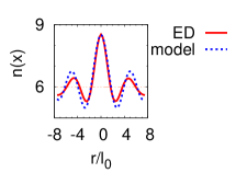
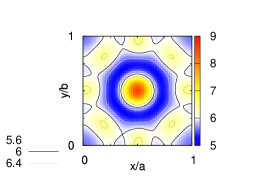
(a)	(b)

Figure 1: Right: electron density $n(x,y)$ of the Laughlin state in a square with periodic boundary conditions under the influence of a single point impurity of intermediate strength. Six electrons (implying $a=b=10.6\ell_{0}$ to ensure $\nu=\frac{1}{3}$), $V_{0}=0.3e^{2}/(4\pi\varepsilon\ell_{0})$, $\sigma=1.0\ell_{0}$ (Eq. 1). Left: section of $n(x,y)$ along the diagonal (ED), comparison to the simple model based on $\chi(\vec{q})=\delta(|\vec{q}-q_{0}|)$, $q_{0}\ell_{0}=1.4$, see text.

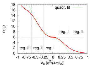
Figure 2: Compression of the Laughlin state by a point impurity measured by the local density at $r_{0}$ (Eq. 1). Strength of the impurity $V_{0}$ is divided into regions I, II and III described in text.

As a tool of study we use the exact diagonalization (ED) with Coulomb-interacting electrons on a toruschakraborty:1995 ; yoshioka:2002 ; yoshioka:06:1984 . Contrary to the spherical geometry, a point impurity

$$V({\vec{r}})=V_{0}\exp{[-({\vec{r}}-{\vec{r}_{0}})^{2}/\sigma^{2}]}$$ (1)

does break geometric symmetries on the torus described by the quantum numbershaldane:11:1985 $\mathbf{k}=(k_{x},k_{y})$. This makes the study more difficult from the computational view (large dimension of the Hilbert space) but it also gives the system the full freedom of choosing the ground state. The density response $n(x,y)$, Fig. 1, clearly follows the impurity form (rotationally symmetric) on short ranges and it is deformed by the periodic boundary conditions on distances comparable to the size of the elementary cellchakraborty:1995 $a=b=\sqrt{2\pi N_{m}}\ell_{0}$. Here $\ell_{0}$ is the magnetic length and $N_{e}$, $N_{m}$ are the number of electrons and the number of magnetic flux quanta.

It should be noted that the oscillations in the density response $n(x,y)$ are not of the Friedel type known in a Fermi gasashcroft:1976 ; stern:04:1967 ; stern:11:1967 which occur as interferences at the edge of the Fermi–Dirac distribution at the Fermi wave vector. In the regime of linear response, the oscillations like in Fig. 2 can be described up to a very good precision by a model dielectric response function $\chi(\vec{q})=\delta(|\vec{q}|-q_{0})$. This is an approximation based on the observation that the magnetoroton minimum at $q_{0}\ell_{0}\approx 1.4$ is the lowest no-spinflip excitation at $\nu=\frac{1}{3}$. A more realistic $\chi(\vec{q})$ based on the single mode approximation was given by MacDonaldmacdonald:03:1986 and we recall that it is very different from $\chi(\vec{q})$ of a Fermi gasashcroft:1976 ; macdonald:03:1986 .

It was noted already by Rezayi and Haldanerezayi:11:1985 that the form of the density response calculated for the linear regime, $\Delta n(r)\propto J_{0}(rq_{0})$, remains almost unchanged even in the non-linear regime $|V_{0}|\gg E_{g}$. This statement applies also for point impurities on a torus with two comments. (a) The density profile predicted by the linear response calculation is correct also outside the linear regime (large $V_{0}$), but not all the way up to $V_{0}\to\infty$ as on a sphererezayi:11:1985 . (b) This density profile $n$ is also correct when $V_{0}$ drops into the $\Delta n(r_{0})\propto V_{0}^{2}$ regime. However, it may be masked by density modulation due to finite size effects in small systemsvyborny:2005 .

On a torus at at $\nu=1/3$, the CM wavefunctions span a three-dimensional spacehaldane:11:1985 . States in a homogeneous system can be factorized into a CM and relative parts, $\Psi=\Psi_{CM}\psi_{rel}$. Even the incompressible Laughlin ground state is thus triply degenerate on the torus and the electron density in this state strongly depends on which linear combination we choose for its $\Psi_{CM}$. Impurities lift the degeneracy but the splitting $\Delta E$ remains very small, $\Delta E\ll V_{0}\lesssim E_{g}$. Density responses in each state $\Delta n_{V_{0}}=n_{V_{0}}-n_{V_{0}\to 0}$ are not identical but differences and vanish with increasing system size. The roles of the three states can be interchanged by moving $\vec{r}_{0}$, Eq. 1. We always chose the state with lowest energy for plots in this article.

We attribute the $\Delta n(r_{0})\propto V_{0}^{2}$ behaviour to the situation where the CM part of the wavefunction enters as a degree of freedom. Matrix elements of the electron density between two states are proportional to the overlap of their CM parts. In particular, if these are mutually orthogonal, the corrections to the density linear in $V_{0}$ will vanish. For stronger impurity potentials, the CM degree of freedom may be frozen out and linear admixtures to the ground state wavefunction imply linear corrections to the electron density. For electrons on a sphere or impurities discussed in the next section, the CM degree of freedom is never enabled and the density response is linear down to $V_{0}\to 0$.

II Response to a $\delta$-line impurity

Comparing results for different system sizes is essential in finite system studies. To keep such calculations tractable we must return to impurities which preserve some symmetries of the system. The $\delta$-line impurity

$$V_{\delta\mbox{--line}}(x,y)=V_{0}\delta(x-x_{0})\,,$$

in a rectangle with periodic boundary conditions has a similar position as a point impurity on a sphere. The former conserves translational symmetry along $y$, the latter conserves projection of the angular momentum to one axis. A straightforward consequence is that a $\delta$-line impurity does not mix the center-of-mass degenerate ground states on a torus. From the viewpoint of perturbation theory, the ground states are then non-degenerate and the regime of $\Delta n(r_{0})\propto V_{0}^{2}$, Fig. 2, is thus absent. Consequently, $\Delta n(r_{0})$ is linear in $V_{0}$ even for $|V_{0}|\lesssim E_{g}$.

Throughout the rest of the article we will only use the $\delta$–line impurity with a strength of $V_{0}=0.01e^{2}/(4\pi\varepsilon\ell_{0})$ which is for all studied states $\ll E_{g}$. Calculated responses then provide information on the relative robustness of the different states (note however that the response is not a property of the ground state alone but depends also on low excited states). The form of the response is found to be independent on $V_{0}$ as long as $|V_{0}|\lesssim E_{g}$. Potentially, $V_{\delta\mbox{--line}}$ may be useful in studies of domain walls but we do not follow this aim in this articlevyborny:2005 .

Turning to the $\frac{1}{3}$ Laughlin state, a linear-response analysis as in Ref. rezayi:11:1985 yields $\Delta n(x,y)\propto\exp(-x^{2}/s^{2})$ for $x_{0}=0$. It is noteworthy that the form of $\Delta n(x,y)$ should be now governed by the width $s$ of the peak of $\chi(\vec{q})$ rather than by its position $q_{0}$. However, this simple model of $\chi(\vec{q})$ seems to fail as the Laughlin state density response is again oscillatory, Fig. 3, yet with different period than for point impurities (dotted line).

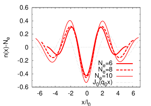
Figure 3: The Laughlin state responding to a $\delta$-line repulsive impurity. Responses in systems of different sizes are compared among each other and also to the linear response modelrezayi:11:1985 for point impurities, cf. Fig. 1.

Keeping in mind the spin degree of freedom, an impurity can principally be one of the following three different types ($\delta_{\sigma\uparrow}$ is a projector to states with spin $\uparrow$)

$$H_{imp}=E_{imp}\sum_{i=1}^{N_{e}}V(\vec{r}_{i})\otimes\left\{\begin{array}[]{ll}\delta_{\sigma_{i}\uparrow}+\delta_{\sigma_{i}\downarrow}&\mbox{ 'EI'}\\ \delta_{\sigma_{i}\uparrow}-\delta_{\sigma_{i}\downarrow}&\mbox{ 'MI'}\\ \delta_{\sigma_{i}\uparrow}&\mbox{ 'DP'}\end{array}\right.\,.$$ (2)

The electric potential impurity (EI) stands for a simple potential modulation ($\delta_{\sigma_{i}\uparrow}+\delta_{\sigma_{i}\downarrow}=1$), the magnetic impurity (MI) can be viewed as a spatially varying Zeeman field [$V(\vec{r}_{i})\otimes(\delta_{\sigma_{i}\uparrow}-\delta_{\sigma_{i}\downarrow})\propto B_{z}(\vec{r}_{i})\sigma^{z}_{i}$] and the delta–plus impurity (DP) acts as a potential modulation seen only by spin–up electrons. The last type of impurity, DP, is less likely to occur in physical systems, however, it is helpful to understand the mechanisms governing inner structure of the states in study.

It is important to check whether the response does not decay with increasing system size. Such a behaviour may imply that the response vanishes in large enough systems. However, in most of cases we find even a slight increase of the density response $\Delta n(r)$, e.g. Fig. 2. Exceptions from this will be explicitly stated.

II.1 Electric potential impurity (EI)

The polarized states of $\frac{1}{3},\frac{2}{3}$ and $\frac{2}{5}$ respond all very similarly to a weak potential impurity. The singlet states at $\frac{2}{5}$ and $\frac{2}{3}$ respond more weakly and this is particularly apparent in the latter case. We give details on this observation in this Section and then focus on the $\frac{2}{3}$ singlet state in the succeeding Sections.

It is not surprising that the Laughlin state and the polarized state at $\frac{2}{3}$ have a similar response. They are particle hole conjugates ($\nu$ and $1-\nu$) and even though inhomogeneities break the symmetry of the Hamiltonianvyborny:2005 , the effect appears extremely weak on the scale of Fig. 4. Also the $\frac{2}{5}$ polarized state and the Laughlin state show almost the same response, Fig. 4. This applies both to its strength and the position of the first maximum (or node). Such a finding is non-trivial as the two states correspond to different filling factors in the CF picture. It is also non-trivial from the analogy between $\frac{2}{5}$ and $\frac{2}{3}$. Here both states correspond to $\nu^{*}=2$ but the wavefunctions show different correlations on the electronic levelvyborny:2005 .

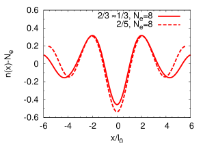
Figure 4: Response of the polarized $\frac{2}{5}$ and $\frac{2}{3}$ (almost identical to that of $\frac{1}{3}$) states to a $\delta$-line EI. Eight electrons considered, $V_{0}=0.01e^{2}/(4\pi\varepsilon\ell_{0})$.

Now turn to the singlet GS, Fig. 5. The $\frac{2}{5}$ singlet seems to respond less strongly compared to the polarized state but the difference is small, Fig. 5b (crosses and the thin line). The difference between the polarized and singlet state at $\frac{2}{3}$, however, is striking, Fig. 5a. Measured by $\Delta n(r_{0})$, the singlet appears about four times more robust than the polarized state.

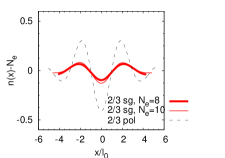
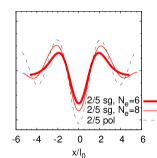
(a) $\frac{2}{3}$ singlet	(b) $\frac{2}{5}$ singlet

Figure 5: The singlet states subject to a potential impurity. Response of the polarized states (thin dashed lines) is shown for comparison.

These findings can neither be completely explained with the intuition of non-interacting CFs nor purely on the basis of the numerically calculated gaps. For the former, we would expect both the $\frac{2}{5}$ and $\frac{2}{3}$ singlet to have the same response as the Laughlin state. In all three states all CFs reside in the lowest CF Landau level and they are excited to the first CF LL by the impurity. On the other hand, the CF intuition is correct for the $\frac{2}{3}$ and $\frac{2}{5}$ polarized states.

Regarding the gap energies it is also unexpected that the $\frac{2}{3}$ spin singlet seems more robust than the polarized state whose gap is larger. An explanation for the stability of the singlet state must therefore lie in the structure of the wavefunctions rather than in the spectrum.

III Spin pairing in the $\frac{2}{3}$ singlet state

The density–density correlation functions provide an alternative view at the internal structure of a many body state $|\Psi\rangle$. With spin degree of freedom, there are three distinct types denoted by $g_{\uparrow\uparrow}$(r), $g_{\downarrow\downarrow}(r)$ and $g_{\uparrow\downarrow}(r)$. With $\delta_{\sigma\uparrow}$ being a projector on spin up single-electron states, the first one is defined as $\langle\Psi|\delta(r-r^{\prime}-r^{\prime\prime})\delta_{\sigma^{\prime}\uparrow}\delta_{\sigma^{\prime\prime}\uparrow}|\Psi\rangle$, the others analogously.

The $\nu=\frac{2}{3}$ singlet state displays remarkable structures in these spin-resolved correlations, Fig. 6. While $g_{\uparrow\uparrow}(r)$ has a pronounced shoulder around $r\approx 2\ell_{0}$, the unlike spins have a strong correlation maximum near $3.5\ell_{0}$. Even though not shown in Fig. 6, this was checked for several different system sizes and the above dimensions turned out to be always the same. Note that these structures are significantly stronger than in the casekamilla:11:1997 ; vyborny:2005 of the Laughlin state at $\nu=\frac{1}{3}$. We interpret this as a signature of spin pairing: two electrons with opposite spin form an object of the characteristic size of approximatelly three magnetic lengths which is the mean interparticle separation $\sqrt{2\pi/\nu}\ell_{0}\approx 3.1\ell_{0}$. Qualitatively the same behaviour was found in the $\frac{2}{5}$ singlet statevyborny:2005 .

Moreover, combining the correlation functions above into a spin-unresolved onecomm:04 , $g_{*}(r)=g_{\uparrow\uparrow}+g_{\uparrow\downarrow}$, we arrive at a result strongly reminiscent of the completely filled lowest Landau level (i.e. the ground state at $\nu=1$), Fig. 7. Such a state is characteristic by a simple correlation hole at $r=0$ passing over monotonously to a constantgirvin:07:1999 : $g_{\nu=1}(r)=1-\exp(-r^{2}/2\ell_{0}^{2})$. Surprisingly, however, the correlation hole found in $g_{*}(r)$ corresponds to $g_{\nu=1}$ with $\ell_{0}^{2}$ replaced by $2\ell_{0}^{2}$ with a rather good precision (the fit in Fig. 7).

In a finite system with $N_{e}$ electrons, $g_{*}=g_{\nu=1}$ would mean that these electrons form the standard $\nu=1$ state and behave as if they felt $N_{m}=N_{e}$ magnetic flux quanta. With the replacement $\ell_{0}^{2}\to 2\ell_{0}^{2}$ we conclude that the electrons feel only $N_{m}=N_{e}/2$ flux quanta, or that each pair of electrons feels one flux quantum. Based on observations in Fig. 6,7 we suggest that the electrons in the $\frac{2}{3}$ singlet state form pairs of total spin zero with characteristic size of $3\ell_{0}$ and these pairs condense into a state resembling the completely filled lowest Landau level.

The observed robustness of the singlet states against the potential impurities thus may be related to the robust incompressibility of the filled lowest Landau level, possibly helped also by the fact that the relevant particles are not single electrons but rather electron pairs. We now proceed with the investigation of the spin singlet states keeping in mind this picture providing a guidance at the interpretation.

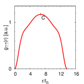
Figure 6: Correlations between like spins and unlike spins in the $\frac{2}{3}$ singlet state. Ten electrons in a square elementary cell (C marks its centre), $g(r)$ along its diagonal is shown. Note the maximum in $g_{\uparrow\downarrow}(r)$ around $3.4\ell_{0}$.

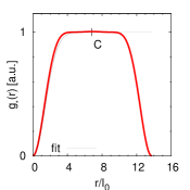
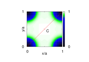
Figure 7: Data of Fig. 6 combined into a spin-unresolved correlation function of the $\frac{2}{3}$ singlet state closely resemble the completely filled lowest Landau level with $N_{e}/2$ particles (the fit). The $g_{*}(r)$ in the whole elementary cell and a section along the diagonal are shown.

III.1 Magnetic impurity (MI)

A magnetic impurity creates a relatively strong spin polarization $p(x)=[n_{\uparrow}(x)-n_{\downarrow}(x)]/n(x)$ of the singlet states, Fig. 8c,d. The density of electrons with spin $\uparrow$ at $x=0$ decreases by $40\%$ and $30\%$ for $\frac{2}{5}$ and $\frac{2}{3}$, respectively. On the other hand, a potential impurity of the same strength $V_{0}$ changes the total density of these states only by $5\%$ and $1.5\%$, Fig. 5.

This observation is compatible with the concept of singlet pairs forming a $\nu=1$ state ($\frac{2}{3}$ singlet). While the potential impurity forces the whole unwieldy pairs to rearrange, it is relatively easy to polarize the pairs without moving their centre of mass. In terms of the many-body states, the weak density response suggests that the correlations in the ground state are similar to those of low lying excited states.

Several remarks should be added. (a) Magnetic impurity changes not only the polarization but also the density, Fig. 8a,b. This effect is proportional to $V_{0}^{2}$ and it is a consequence of that the density and spin density operators do not commute within the lowest Landau levelgirvin:07:1999 . Regardless of the sign of $V_{0}$, the density always increases at the impurity position. (b) The polarization profiles show only one node in our finite systems, Fig. 8c,d. Characteristic length related to screening of magnetic impurities, if present at all, is therefore probably rather large. (c) The $\frac{2}{5}$ singlet state with a magnetic impurity is the only case in this work where increasing the system size leads to a notably smaller density (and also polarization) response.

2/3	2/5
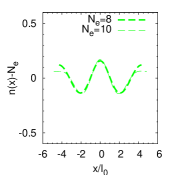
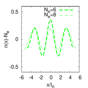
(a)	(b)
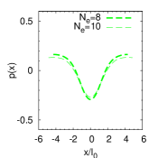
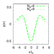
(c)	(d)

Figure 8: Density (a,b) and polarization (c,d) response of the $\frac{2}{3}$ and $\frac{2}{5}$ singlet states to a magnetic impurity.

III.2 Delta plus impurity (DP)

Finally we investigate the $\frac{2}{3}$ singlet state subject to the ’delta plus’ impurity, Eq. 2, and found weaker responses than for other types of impurities, Fig. 9. Put into the context of our singlet-pair incompressible state this finding reflects the strong correlations within the pair.

We point out that the response to a DP impurity cannot be derived only from the knowledge of responses to a potential and to a magnetic impurity even though EI+MI=2$\times$DP on the level of the Hamiltonian, Eq. 2. We find that the density responses to a potential impurity (EI) and the DP impurity are in ratio $\approx 4:1$, Fig. 9a while the polarization responses to the magnetic impurity (MI) and the DP are $\approx 3:1$, Fig. 9b. The both being more than $2:1$ means that the capability of the individual spin species to answer to external perturbations is suppressed, hence suggesting that their mutual correlation is strong. It is also worth of recalling that the response of the $\frac{2}{3}$ singlet state to a DP is thus more than an order of magnitude smaller than the one of the Laughlin state, Fig. 9a. A naive interpretation of $\nu^{*}=2$, for example, as of two independent $\nu^{*}=1$ systems (corresponding to Laughlin wavefunctions) with different spins therefore fails utterly.

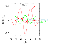
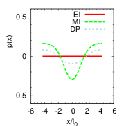
(a)	(b)

Figure 9: Density (a) and polarization (b) response to all three types (Eq. 2) of $\delta$-line impurities acting on the $\frac{2}{3}$ singlet ($N_{e}=8$). Density response of the Laughlin state to a potential impurity is shown for comparison in (a) by the thin line.

IV Summary

We find that the polarized $\nu=\frac{1}{3}$, $\frac{2}{3}$ and $\frac{2}{5}$ states all respond similarly to isolated impurities, represented in this paper by a weak $\delta$-line impurity. Since $\frac{2}{5}$ gives slightly different results than the other two systems we conclude that the particle-hole conjugation ($\frac{1}{3}$ and $\frac{2}{3}$) is a stronger link than the reversal of the effective field in the composite fermion picture ($\frac{2}{3}$ and $\frac{2}{5}$).

The singlet states react differently: both $\frac{2}{3}$ and $\frac{2}{5}$ respond quite unequally and more weakly to an electric potential impurity than $\frac{1}{3}$. In particular, $\frac{2}{3}$ gives a much weaker response than $\frac{1}{3}$. This was unexpected because the Laughlin state has the largest incompressibility gap. The spin-resolved and spin-unresolved density-density correlation functions of the $\frac{2}{3}$ singlet state suggest that electrons in it appear in zero-spin pairs with characteristic size of $3$ magnetic lengths and these form a full-Landau-level-like state. High polarizability by magnetic impurities and a relatively small effect of impurities affecting only one spin species are compatible with this interpretation.

The authors acknowledge support from the following grants: AV0Z10100521 of the Academy of Sciences of the Czech Republic (KV), LC510 of the Ministry of Education of the Czech Republic (KV), and SFB 508 Quantenmaterialien.

References

- (1) X. Wan, D.N. Sheng, E.H. Rezayi, K. Yang, R.N. Bhatt, and F.D.M. Haldane, Phys. Rev. B 72, 075325 (2005).
- (2) T. Chakraborty and Pietiläinen, P. The Quantum Hall Effects. Springer, Berlin, second edition, 1995.
- (3) J. Martin, S. Ilani, B. Verdene, J. Smet, V. Umansky, D. Mahalu, D. Schuh, G. Abstreiter, A. Yacoby. Science, 305:980, 2004.
- (4) I.V. Kukushkin, K.v. Klitzing, and K. Eberl. Phys. Rev. Lett., 82:3665, 1999.
- (5) K. Výborný, O. Čertík, D. Pfannkuche, D. Wodziński, A. Wójs, and J.J. Quinn. Phys. Rev. B., 75:045434, 2007.
- (6) E. Mariani, N. Magnoli, F. Napoli, M. Sassetti, and B. Kramer. Phys. Rev. B., 66:241303, 2002.
- (7) M. Merlo, N. Magnoli, M. Sassetti, and B. Kramer. Phys. Rev. B., 71:155307, 2005.
- (8) V.M. Apalkov, T. Chakraborty, P. Pietiläinen, and K. Niemelä. Phys. Rev. Lett., 86:1311, 2001.
- (9) G. Murthy. Phys. Rev. Lett., 84:350, 2000.
- (10) F.C. Zhang, V.Z. Vulovic, Y. Guo, and S. Das Sarma. Phys. Rev. B, 32:6920, 1985.
- (11) E.H. Rezayi and F.D.M. Haldane. Phys. Rev. B, 32:6924, 1985.
- (12) O. Heinonen (Ed.), Composite Fermions (World Scientific, Singapore, 1998).
- (13) G. Dev and J.K. Jain. Phys. Rev. Lett., 69:2843, 1992.
- (14) K. Výborný. Spin in fractional quantum Hall systems. PhD thesis, Universität Hamburg, 2005 (www.sub.uni-hamburg.de/opus/volltexte/2005/2553); K. Výborný, Ann. Phys. (Leipzig) 16 [2], 87 (2007).
- (15) D. Yoshioka. The Quantum Hall Effect. Springer, Berlin, 2002.
- (16) D. Yoshioka. Phys. Rev. B, 29:6833, 1984.
- (17) F.D.M. Haldane. Phys. Rev. Lett., 55(20):2095, 1985.
- (18) N.W. Ashcroft and N.D. Mermin. Solid State Physics. Saunders College, Philadelphia, 1976.
- (19) F. Stern. Phys. Rev. Lett., 18:546, 1967.
- (20) F. Stern and W.E. Howard. Phys. Rev., 163:816, 1967.
- (21) A.H. MacDonald, K.L. Liu, S.M. Girvin, and P.M. Platzman. Phys. Rev. B, 33:4014, 1986.
- (22) R.K. Kamilla, J.K. Jain, and S.M. Girvin. Phys. Rev. B, 56:12411, 1997.
- (23) More precisely, we used to account for the finite size of the system. and is the number of electrons with spin up and spin down, respectively.
- (24) S.M. Girvin, cond-mat/9907002, (1999).