Microwave photoconductivity of a 2D electron gas:
Mechanisms and their interplay at high radiation power

Abstract

We develop a systematic theory of microwave-induced oscillations in the magnetoresistivity of a two-dimensional electron gas, focusing on the regime of strongly overlapping Landau levels. At linear order in microwave power, two novel mechanisms of the oscillations (“quadrupole” and “photovoltaic”) are identified, in addition to those studied before (“displacement” and “inelastic”). The quadrupole and photovoltaic mechanisms are shown to be the only ones that give rise to oscillations in the nondiagonal part of the photoconductivity tensor. In the diagonal part, the inelastic contribution dominates at moderate microwave power, while at elevated power the other mechanisms become relevant. We demonstrate the crucial role of feedback effects, which lead to a strong interplay of the four mechanisms in the nonlinear photoresponse and yield, in particular, a nonmonotonic power dependence of the photoconductivity, narrowing of the magnetoresonances, and a nontrivial structure of the Hall photoresponse. At ultrahigh power, all effects related to the Landau quantization decay due to a combination of the feedback and multiphoton effects, restoring the classical Drude conductivity.

I Introduction

In recent years, the nonequilibrium properties of quantum Hall systems in a moderate perpendicular magnetic field $B$ have become a subject of intense experimentalzudov01 ; Ye01 ; yang02 ; mani02 ; zudov03 ; yang03 ; dorozhkin03 ; willett03 ; B-periodic ; zudov04 ; du04 ; mani04 ; maniHall ; Studenikin04 ; Kovalev ; mani05 ; polarization ; studenikin05 ; studenikin06 ; bykov1 ; bykov2 ; parr B ; antidot ; dorozhkinINTRA ; bichrom ; multi ; dorozhkin06 ; inelasticDC ; strongDC ; ACDC and theoreticalandreev03 ; ryzhii ; durst03 ; dmitriev03 ; Raikh03 ; shi ; ryzhii03 ; leiliu03 ; VA ; short ; classical ; compress ; michailov04 ; park ; lee ; Raikh04 ; Lyapilin1 ; ryzhii04 ; falkoprl ; long ; Halperin ; Balents ; vonoppen1 ; vonoppen2 ; torres05 ; leiliu05 ; Volkov ; michailov04a ; falkoprb ; dietel ; torres06 ; Kashuba06 ; Lyapilin2 ; leiliumulti ; leiliubichrom ; 2componentDC ; Auerbach ; crossover research (for review see Refs. Fitzgerald, ; Girvin, ; Lyap, ; Durst06, ). Much attention has been attracted to the experimental discovery of a novel type of $1/B$-periodic resistivity oscillations which arise in these systems under microwave illumination.zudov01 ; Ye01 Remarkably, it was demonstrated soon after the first experiments that at higher radiation power the minima of the oscillations evolve into novel “zero-resistance states” (ZRS).mani02 ; zudov03

As was shown in Ref. andreev03, , the ZRS can be understood as a direct consequence of the oscillatory photoconductivity (OPC), provided the latter may become negative. Independently of the microscopic origin of the oscillations, the negative OPC signifies an instability leading to the formation of spontaneous-current domains, which in turn yields the vanishing of the observable resistance.

Unlike the explanation of the ZRS, so far there has been no common agreement as to the microscopic origin of the OPC. The most frequently studied mechanismryzhii ; durst03 ; shi ; ryzhii03 ; leiliu03 ; VA ; park ; lee ; Lyapilin1 ; ryzhii04 ; torres05 ; leiliu05 ; Volkov ; torres06 ; Kashuba06 ; Lyapilin2 ; leiliumulti ; leiliubichrom ; Auerbach of the OPC, suggested long ago in Ref. ryzhii, , implies that the oscillations occur due to complex scattering processes in which electrons simultaneously are scattered off impurities, absorb (emit) microwave quanta, and are displaced along the applied dc electric field. We term this mechanism a “displacement” mechanism. A different mechanism, called here the “inelastic” mechanism, was recently proposed in Ref. dmitriev03, and studied in detail in Refs. short, ; long, (similar ideas were also discussed in Ref. dorozhkin03, ). In the inelastic mechanism, the magnetooscillations of the dc current are generated by a microwave-induced change of the isotropic time-independent part $F_{00}(\varepsilon)$ of the electron distribution function,

$$f(\varepsilon,\varphi,t)=\sum_{\nu n}F_{\nu n}(\varepsilon)\exp(i\nu\varphi+in\omega t)~{},$$ (1.1)

where $\varepsilon$ is the electron energy, $\varphi$ the angle of the quasiclassical momentum, $\omega$ the microwave frequency.

The above mechanisms have much in common. In both of them, the OPC originates from oscillations of the density of states (DOS) $\nu(\varepsilon)$ of disorder-broadened Landau levels with changing $\varepsilon$. Due to the oscillatory $\nu(\varepsilon)$, optical transitions in the system lead to a nonequilibrium correction to the distribution function $f$ which oscillates with both $\varepsilon/\omega_{c}$ and $\omega/\omega_{c}$, where $\omega_{c}$ is the cyclotron frequency. In turn, the $\omega/\omega_{c}$-oscillations of $f$ translate into the observed $\omega/\omega_{c}$-oscillations of the magnetoresistivity.

A crucial difference between the two mechanisms is the following. In the displacement mechanism, the radiation directly affects the first angular harmonic $F_{10}(\varepsilon)$ of the distribution function (and thus the dc current), whereas all effects of the ac and dc fields on the even angular harmonics are neglected. By contrast, in the inelastic mechanism the ac field influences the isotropic part $F_{00}(\varepsilon)$ only. A calculation of the dc response in the resulting state with a modified $F_{00}(\varepsilon)$ yields the OPC. While in the first case the effect on the current is gained directly in every microwave-assisted impurity-induced electron scattering event, in the latter case the effect is accumulated over a long period of time during which the electron diffuses in the field of impurities until it experiences inelastic scattering. At experimentally relevant temperatures $T\sim 1$ K, the inelastic relaxation is governed by electron-electron scatteringsshort ; long with the inelastic relaxation time $\tau_{\rm in}\propto T^{-2}$.

In the linear regime with respect to the microwave power, the contributions to the OPC generated by the displacement and inelastic mechanisms sum up independently. A comparison shows [see Eqs. (16) and (17) of Ref. long, and Eqs. (6) and (11) of Ref. VA, ] that both mechanisms produce the OPC with the experimentally observed phase, period, and $B$-damping of the oscillations. However, the slow inelastic relaxation rate (compared to the rate of electron collisions with impurities, $\tau_{\rm q}^{-1}$) makes the inelastic contribution larger by a factor $\tau_{\rm in}/\tau_{\rm q}\gg 1$. According to the calculation in Ref. long, , $\tau_{\rm in}/\tau_{\rm q}\sim 100$ under the experimental conditions.tauin Apart from the magnitude of the effect, the two contributions are qualitatively different in their dependence on $T$ and polarization of the radiation. In accord with the experiments, the inelastic contribution decreases as $\tau_{\rm in}\propto T^{-2}$ with increasing $T$ and does not depend on the direction of linear polarization of the microwave field. By contrast, the displacement mechanism yields a $T$ independent contribution which depends essentially on the relative orientation of the microwave and dc fields. Despite the above arguments, in a number of recent works park ; lee ; Lyapilin1 ; ryzhii04 ; torres05 ; leiliu05 ; Volkov ; torres06 ; Kashuba06 ; Lyapilin2 ; leiliumulti ; leiliubichrom ; Auerbach on this subject the inelastic mechanism has not been taken into account.

In this work, we perform a systematic study of all relevant contributions to the OPC both in the linear regime and in several nonlinear regimes which emerge with increasing microwave power. On the experimental side, this work has been motivated by a number of interesting nonlinear phenomena observed in recent experiments.bichrom ; multi ; dorozhkin06 ; inelasticDC ; strongDC ; ACDC From the theoretical point of view, a unified approach to the problem is necessary since at high microwave power the interplay of the inelastic and displacement mechanisms becomes essentially important. We show that the different mechanisms of the OPC strongly affect each other due to feedback effects already at moderate power levels which are easily accessible in the experiment. In particular, while in the linear regime the displacement and inelastic contributions to the OPC add up in phase, in the regime of a “saturated inelastic contribution” (SIC) the displacement contribution changes its sign, which leads to a nonmonotonic behavior of the photoresponse (still dominated by the inelastic contribution) with growing microwave power. In the ultrahigh power regime, all contributions to the dc conductivity that are related to the Landau quantization decrease with increasing power due to a competition between the feedback and multiphoton effects. As a result, the oscillations of the photoresponse vanish and the classical Drude conductivity tensor is restored in the limit of high radiation power.

On top of the nonlinear interplay between the inelastic and displacement mechanisms, we find two novel mechanisms leading to the OPC, “quadrupole” and “photovoltaic”. In the quadrupole mechanism, the microwave radiation leads to excitation of the second angular harmonic $F_{20}$ of the distribution function. The dc response in the state with nonzero $F_{20}$ yields an oscillatory contribution to the Hall part of the photoconductivity tensor which violates Onsager symmetry. In the photovoltaic mechanism, a combined action of the microwave and dc fields produces non-zero temporal harmonics $F_{21}$ and $F_{01}$, so that the distribution function (1.1) acquires oscillatory time dependence. The ac response in the resulting state with excited $F_{21}$ and $F_{01}$ contributes to both the longitudinal and Hall parts of the OPC. Provided $\tau_{\rm in}/\tau_{\rm q}\gg 1$, the inelastic mechanism still gives the dominant contribution to the diagonal part of the photoconductivity tensor. However, the quadrupole and photovoltaic mechanisms are the only ones yielding oscillatory corrections to the Hall part.

The paper is organized as follows. In Sec. II we formulate the problem and overview the main steps in the derivation of the quantum kinetic equation obtained in Ref. VA, . Using this kinetic equation, in Sec. III we put forward a general classification of contributions to the photoconductivity at first order in the microwave power. We discuss here four distinctly different mechanisms of the OPC. In Sec. IV we write down the kinetic equation for the case of strongly overlapping Landau levels, which we focus on hereafter. In Sec. V we calculate the linear photoconductivity. In Secs. VI and VII we analyze several nonlinear regimes the system passes through with increasing microwave power. Namely, in Sec. VI we study the SIC regime at moderate power, driven by feedback effects. In Sec. VII we turn to the interplay of the feedback and multiphoton effects in the regime of ultrahigh microwave power. In Sec. VIII we consider the possibility of experimental observation of the nonlinear effects in the magnetoresistivity measurements. In Sec. IX the range of applicability of the theory is discussed. The main results are summarized in Sec. X.

II 2D electron gas in a classically strong magnetic field under microwave irradiation

Our theory is based on the approach to the problem of kinetics of a 2D electron gas (2DEG) in the presence of magnetic field and radiation that was developed by Vavilov and Aleiner.VA This approach was used for a systematic study of the displacement mechanism of the OPC in Ref. VA, . It was further developed to treat the inelastic mechanism in Ref. long, . Based on controllable approximations, the approach allows us to analytically describe the nonlinear behavior of the system under intense microwave radiation.

II.1 Model and parameters

Let us first specify the model. The relation between the main parameters of our theory, which is also satisfied for the characteristic parameters of the 2DEG studied in the experiments on the OPC, is as follows:

$$\varepsilon_{F}\gg T\,,\,\omega\,,\,\omega_{c}\,,\,\tau^{-1}_{\rm q}\gg\tau^{-1}_{\rm tr}\,,\,\tau^{-1}_{\rm in}~{}.$$ (2.1)

Here $\varepsilon_{F}$ is the Fermi energy, $T$ the temperature, $\omega$ the microwave frequency, $\omega_{c}$ the cyclotron frequency, $\tau_{\rm q}$ and $\tau_{\rm tr}$ the quantum (single-particle) and transport disorder-induced scattering times, respectively, and $\tau_{\rm in}$ the inelastic relaxation time. The conditions (2.1) imply:

• quasiclassical kinetics: the 2D electron states that contribute to transport belong to high Landau levels in a narrow energy strip of width $T$ around the Fermi level, $\varepsilon_{F}\gg T,\omega_{c}$;

• predominantly small–angle scattering (smooth disorder), $\tau_{\rm tr}\gg\tau_{\rm q}$;

• classically strong magnetic field, $\omega_{c}\tau_{\rm tr}\gg 1$;

• pronounced oscillations in the DOS due to the Landau quantization, $\omega_{c}\tau_{\rm q}\sim 1$.

In the high-mobility structures used in the experiment a smooth random potential in the plane of the 2DEG was created by remote donors separated from the 2DEG by a spacer of width $\xi/2\gg k_{F}^{-1}$, where $k_{F}$ is the Fermi momentum. The Fourier transform of the correlation function of the random potential,

$$W(q)=W(0)\,e^{-q\xi}~{},$$ (2.2)

falls off exponentially for momentum transfers $q\gg\xi^{-1}$, leading to $\tau_{\rm q}/\tau_{\rm tr}=(k_{F}\xi)^{-2}\ll 1$, where the quantum and transport scattering times in zero magnetic field are given by

$$\frac{1}{\tau_{\rm q}}=\int\limits^{\infty}_{0}{dq\over 2\pi}\,{W(q)\over 2v_{F}}~{},$$ (2.3)

$$\frac{1}{\tau_{\rm tr}}=\int\limits^{\infty}_{0}{dq\over 2\pi}\,{W(q)\over 2v_{F}}\left(\frac{q}{2k_{F}}\right)^{2}~{}.$$ (2.4)

Effects of the smooth disorder on the spectral and transport properties of 2D electrons occupying high Landau levels can be properly described by the self-consistent Born approximation (SCBA),Ando provided that $\xi$ does not exceed the magnetic lengthRaSha (which is the case for the relevant magnetic fields in most of the experiments).

II.2 Quantum Boltzmann equation

Using the SCBA under the conditions listed in Eq. (2.1), Vavilov and Aleiner derived the quantum Boltzmann equation (QBE),VA which is the starting point of our calculation. The derivation of the QBE includes a few key steps which we highlight below.

• Moving coordinate frame.

  The initial problem of electron kinetics in the quantizing magnetic field and the external (microwave + dc) electric field ${\bf E}(t)$ in the presence of static impurities is reduced to a problem of kinetics in the presence of “dynamic” impurities, whose potential is $t$ dependent, by changing to a moving coordinate frame $\mbox{\boldmath$r$}\rightarrow\mbox{\boldmath$r$}-\mbox{\boldmath$\zeta$}(t)$, where $\mbox{\boldmath$\zeta$}(t)$ obeys

  $$\partial_{t}\mbox{\boldmath$\zeta$}(t)=\left(\frac{\partial_{t}-\omega_{c}\hat{\varepsilon}}{\partial_{t}^{2}+\omega_{c}^{2}}\right)\frac{e{\bf E}(t)}{m_{e}}~{},$$

  $$\hat{\varepsilon}_{xy}=-\hat{\varepsilon}_{yx}=1~{}.$$ (2.5)

  All effects of the external electric field are now included in the time dependence of $\mbox{\boldmath$\zeta$}(t)$. The transformation (2.5), which is particularly convenient for treating the external electric field nonperturbatively, is equivalent to the transformation to Floquet states used in a number of workspark ; lee ; Lyapilin1 ; torres05 ; Volkov ; Kashuba06 ; Lyapilin2 ; Auerbach on the OPC.

• Keldysh equations within the SCBA.

  Within the SCBA, the Green’s functions $\hat{G}^{(\alpha)}$ and the self-energies $\hat{\Sigma}^{(\alpha)}$ [$(\alpha)\to R,A,K$ refers to the retarded, advanced, and Keldysh components, respectively] are related to each other as

  $$\hat{\Sigma}^{(\alpha)}_{21} = \int\!\frac{d^{2}q}{(2\pi)^{2}}\,W(q)\,e^{-i\mbox{\boldmath$q$}\mbox{\boldmath$\zeta$}_{21}}$$ (2.6)

  $$\times \left[e^{i\mbox{\boldmath$q$}\hat{\mbox{\boldmath$r$}}}\hat{G}^{(\alpha)}e^{-i\mbox{\boldmath$q$}\hat{\mbox{\boldmath$r$}}}\right]_{21}~{},$$

  where the subscript (21) denotes the times $t_{2}$ and $t_{1}$ on the Keldysh contour and $\mbox{\boldmath$\zeta$}_{21}=\mbox{\boldmath$\zeta$}(t_{2})-\mbox{\boldmath$\zeta$}(t_{1})$.

• Quasiclassical approximation.

  Most importantly, using the conditions (2.1), Vavilov and Aleiner reduced Eq. (2.6) to a simpler quasiclassical equation in the “action-angle” representation:

  $$\Sigma^{(\alpha)}_{21}(\varphi)=-i\hat{\cal K}_{21}\,g^{(\alpha)}_{21}(\varphi)~{},$$ (2.7)

  $$g^{(\alpha)}_{21}(\varphi)\equiv i\omega_{c}\sum_{k}\hat{G}^{(\alpha)}_{21}(\hat{n}+k;\,\hat{\varphi})~{},$$ (2.8)

  where the operators $\hat{n}$ and $\hat{\varphi}$ are canonically conjugated, $[\hat{n},\hat{\varphi}]=-i$. The eigenvalues of $\hat{n}$ and $\hat{\varphi}$ are the Landau level index and the angle coordinate of the momentum, respectively. The explicit expression for the linear operator $\hat{\cal K}$ is given below in Sec. II.3.

A significant difference between Eqs. (2.6) and (2.7) is that for high Landau levels the self-energy becomes $\hat{n}$ independent. It follows that the distribution function $\hat{f}$, defined in the usual way by

$$\hat{G}^{R}-\hat{G}^{A}-\hat{G}^{K}=2\,[\,\hat{G}^{R}\hat{f}-\hat{f}\hat{G}^{A}\,]~{},$$ (2.9)

commutes with $\hat{\varphi}$. Accordingly, the operator $\hat{\varphi}$, which enters Eq. (2.7) and the impurity collision integral

$$i\,{\rm St}_{\rm im}\{f\}=\hat{\Sigma}^{R}\hat{f}-\hat{f}\hat{\Sigma}^{A}+{1\over 2}(\hat{\Sigma}^{K}+\hat{\Sigma}^{A}-\hat{\Sigma}^{R})~{},$$ (2.10)

can be treated as a $c$–number. Substitution of Eqs. (2.7) and (2.8) into Eqs. (2.9) and (2.10) leads to the following quantum kinetic equation:

$${\cal L}\{f\} = {\rm St}_{\rm im}\{f\}$$ (2.11)

$${\cal L}\{f\}_{21} = (\partial_{t}+\omega_{c}\partial_{\varphi})f_{21}-{\rm St}_{\rm in}\{f\}_{21}~{},$$ (2.12)

$${\rm St}_{\rm im}\{f\}_{21} = \int\!dt_{3}\,\left[\,\hat{\cal K}_{21}(g_{23}^{R}f_{31}-f_{23}g_{31}^{A})\right.$$ (2.13)

$$- \left.f_{31}\hat{\cal K}_{23}g_{23}^{R}+f_{23}\hat{\cal K}_{31}g_{31}^{A}\,\right]~{}.$$

Here

$$t=(t_{1}+t_{2})/2$$ (2.14)

is the “center-of-mass” time. The inelastic collision integral ${\rm St}_{\rm in}\{f\}_{21}$ accounts for electron–electron scattering and for coupling to a thermal (phonon) bath.

The spectrum of the problem is found from the coupled set of Eq. (2.7) and the equation of motion

$$\left(i{\partial\over{\partial t_{2}}}-\omega_{c}\hat{n}\right)\hat{G}^{R}_{21}(\hat{n},\,\hat{\varphi})=\frac{\delta(t_{2}-t_{1})}{2\pi}$$

$$+\int_{t_{1}}^{t_{2}}\!dt_{3}\,\hat{\Sigma}^{R}_{23}(\hat{\varphi})\,\hat{G}^{R}_{31}(\hat{n},\,\hat{\varphi})~{}.$$ (2.15)

Altogether, Eqs. (2.7), (2.11), and (2.15) determine both the spectrum and the distribution function. The dc current in the presence of microwave radiation is then given according to Eq. (3.30) of Ref. VA, by

$$\overline{\bf j}=\overline{\bf j}_{d}+\overline{\bf j}_{nd}~{},$$ (2.16)

$$\overline{\bf j}_{nd}=en_{e}\,\overline{\partial_{t}\mbox{\boldmath$\zeta$}(t)}~{},$$ (2.17)

$$\overline{\bf j}_{d}=-2ep_{F}\left\langle{\cos\varphi\choose\sin\varphi}\,2{\rm Re}\int\!d\tau\,\overline{g^{R}_{t,\,t+\tau}f_{t+\tau,\,t}}\right\rangle~{},$$

(2.18)

where ${\bf j}_{nd}$ and ${\bf j}_{d}$ stand for the nondissipative and dissipative components of the current, respectively, and $n_{e}$ is the electron concentration. Here and below, the bar denotes time averaging over the period of the microwave field in the stationary state, the angular brackets denote averaging over the angle $\varphi$.

II.3 Kernel of the QBE

To complete the formulation of the model, we now specify the kernel ${\hat{\cal K}}$ in Eqs. (2.7) and (2.11). According to Ref. VA, , it is can be represented as

$${\hat{\cal K}}_{21} = {1\over 2\tau_{\rm q}}\int\limits_{-\infty}^{\infty}\!dx\,\exp\left(\frac{x\partial_{\varphi}}{2k_{F}\xi}\right)$$ (2.19)

$$\times e^{-|x|-ix{\cal X}_{21}(\varphi)}\exp\left(\frac{x\partial_{\varphi}}{2k_{F}\xi}\right)~{},$$

with all effects of the external electric field ${\bf E}(t)$ being incorporated in the function ${\cal X}_{21}(\varphi)\propto\mbox{\boldmath$\zeta$}_{21}\propto{\bf E}$. Specifically, we parametrize ${\bf E}(t)$ as

$${\bf E}(t)={\bf E}_{\rm dc}+\frac{E_{\omega}}{\sqrt{2}}\,{\rm Re}\left[\,{s_{-}+s_{+}\choose is_{-}-is_{+}}e^{-i\omega t}\,\right]~{},$$ (2.20)

where ${\bf E}_{\rm dc}$ is the dc electric field, $E_{\omega}$ the amplitude of the microwave field ${\bf E}_{\omega}$, and real $s_{\pm}$ with $s_{+}^{2}+s_{-}^{2}=1$ define elliptical polarization of ${\bf E}_{\omega}$ with the main axes along $x$ and $y$. In particular, $s_{+}=1$ ($s_{-}=1$) corresponds to passive (active) circular polarization, $s_{+}=s_{-}=1/\sqrt{2}$ to linear polarization along the $x$–direction ($\varphi=0$).

Using Eqs. (2.5) and (2.20), ${\cal X}\equiv{\cal X}_{21}(\varphi)$ is written as

$${\cal X} = \frac{\mbox{\boldmath$\zeta$}(t_{2})-\mbox{\boldmath$\zeta$}(t_{1})}{\xi}{-\sin\varphi\choose\cos\varphi}$$ (2.21)

$$= {\cal X}_{\rm dc}+{\cal X}_{\omega}~{},$$

where

$${\cal X}_{\rm dc}=-t_{-}\,\sqrt{\frac{\tau_{\rm q}}{\tau_{\rm tr}}}\,\frac{ev_{F}}{\omega_{c}}\,{\bf E}_{\rm dc}{\cos\varphi\choose\sin\varphi}~{},$$ (2.22)

$${\cal X}_{\omega}=-\sin\frac{\omega t_{-}}{2}\sum_{\pm}\;{\cal E}_{\pm}\cos(\varphi\pm\omega t)~{},$$ (2.23)

$t_{-}=t_{2}-t_{1}$, $t$ is given by Eq. (2.14), and

$${\cal E}_{\pm}=s_{\pm}\,\sqrt{\frac{2\tau_{\rm q}}{\tau_{\rm tr}}}\,\frac{eE_{\omega}v_{F}}{\omega(\omega_{c}\pm\omega)}~{}.$$ (2.24)

After a series expansion in $1/k_{F}\xi\ll 1$ the kernel (2.19) acquires the final form we use below throughout the paper:

$${\cal K} = \tau_{\rm q}^{-1}+{\cal K}_{\bot}+{\cal K}_{j}+{\cal K}_{\varphi}+{\cal O}[(k_{F}\xi)^{-2}]~{},$$ (2.25)

$$\tau_{\rm q}{\cal K}_{\bot} = -{{\cal X}^{2}\over 1+{\cal X}^{2}}~{},$$ (2.26)

$$\tau_{\rm q}{\cal K}_{j} = -i\sqrt{\frac{\tau_{\rm q}}{\tau_{\rm tr}}}\left[\,\partial_{\varphi}\,\frac{{\cal X}}{(1+{\cal X}^{2})^{2}}+\frac{{\cal X}}{(1+{\cal X}^{2})^{2}}\,\partial_{\varphi}\,\right]~{},$$

$$\tau_{\rm q}{\cal K}_{\varphi} = \frac{\tau_{\rm q}}{\tau_{\rm tr}}\,\partial_{\varphi}\,\frac{1-3{\cal X}^{2}}{(1+{\cal X}^{2})^{3}}\,\partial_{\varphi}~{}.$$ (2.28)

Equations (2.25)–(2.28) correspond to Eqs. (3.48) and (3.49) of Ref. VA, . We now turn to a systematic analysis of the QBE, starting with a general classification of various contributions to the OPC at order ${\cal O}(E_{\omega}^{2})$.

III Mechanisms of the oscillatory photoconductivity

In this section we present a general solution to the QBE (2.11) to first order in both the microwave power and the dc electric field. The case of strongly overlapped Landau levels, $\omega_{c}\tau_{\rm q}\ll 1$, on which we focus in this paper will be considered at this order in more detail in Sec. V. Throughout the paper we neglect any effect of the microwave radiation on the functions $g^{R(A)}$ which determine the DOS:

$$\nu(\varepsilon,t)=2\nu_{0}\,{\rm Re}\int\!\frac{d\varphi}{2\pi}\int\!dt_{-}\,e^{i\varepsilon t_{-}}g^{R}_{t+t_{-}/2,\,t-t_{-}/2}(\varphi)~{}.$$ (3.1)

This approximation is well justified in the limit $\omega_{c}\tau_{\rm q}\ll 1$. However, at $\omega_{c}\tau_{\rm q}\sim 1$ the microwave and dc fields may lead to a pronounced modification of the DOS (see Secs. V and VI of Ref. VA, ). A manifestation of the effect of the external electric fields on the DOS in the photoresponse will be discussed elsewhere.separated

III.1 Classical limit

To better understand the role of different terms in the kernel (2.25), it is instructive to look first at the QBE in the classical (with respect to the magnetic field) limit $\omega_{c}\tau_{\rm q}\to 0$. In this limit, the DOS $\nu=\nu_{0}=m/2\pi$ is constant, the functions $g^{R}_{21}=-g^{A}_{21}=\delta(t_{2}-t_{1})/2$, and the collision integral ${\rm St}_{\rm im}\{f\}_{21}=\hat{\cal K}_{21}f_{21}-f_{21}K_{0}$, where $K_{0}=\tau_{\rm q}^{-1}$ results from the action of the operator $\hat{\cal K}_{tt}$ on unity. After the Wigner transformation, Eq. (2.11) reduces to

$$(\partial_{t}+\omega_{c}\partial_{\varphi})f-{\rm St}_{\rm in}\{f\}$$

$$=-\frac{f(\varepsilon)}{\tau_{\rm q}}+\int\frac{d\Omega}{2\pi}\,\hat{K}(\Omega)f(\varepsilon-\Omega)~{}.$$ (3.2)

In the absence of electric fields (${\cal X}=0$), the r.h.s. of Eq. (3.2) is written as $K_{\varphi}f=\tau_{\rm tr}^{-1}\partial_{\varphi}^{2}f$, which describes a diffusive relaxation of the electron momentum in a smooth random potential. This part of the kernel, which is the smallest one in the parameter $1/k_{F}\xi\ll 1$, plays no role in this paper.

The linear response to a small electric field ${\cal X}\ll 1$ is fully governed by the part $\hat{{\cal K}}_{j}$ of the kernel, which is odd in ${\bf E}(t)$. Substituting ${\hat{\cal K}}_{j}$ into Eq. (3.2) immediately gives the Drude formula for the conductivity. The term ${\cal K}_{\bot}$, of zero order in $1/k_{F}\xi\ll 1$, is even in the electric field. It modifies the isotropic part of the distribution function, which leads to the effect of heating. Also, $\hat{{\cal K}}_{\bot}$ is responsible for the electric-field-induced changes in higher even angular harmonics of $f$ (as we show below, this yields additional contributions to the photoconductivity).

It is worth noting that under the standard assumption of an energy–independent $\tau_{\rm tr}$ in the degenerate Fermi gas, all nonlinear (in ${\bf E}_{\rm dc}$ and ${\bf E}_{\omega}$) corrections to the Drude formula vanish to zero at the classical level.classical ; VA In order to get a finite dc photoresponse, one should then include an energy variation of $\tau_{\rm tr}$ around the Fermi level, which is, however, still insufficient to get the oscillatory photoresponse.classical As far as the OPC is concerned, at the classical level it can only come from the non–Markovian electron dynamics in a random potential (“memory effects”). This classical contribution to the OPC (in contrast to the classical contribution to the oscillatory ac conductivity) was shownclassical to be parametrically smaller than the quantum contributions we consider below.

III.2 Quantum mechanisms of the oscillatory photoconductivity

The Landau quantization leads to a periodic modulation of the DOS for high Landau levels, $\nu(\varepsilon)=\nu(\varepsilon+\omega_{c})$, which, as far as the OPC is concerned, essentially modifies the classical picture above. In particular, in the high-temperature limit ($T\gg\omega,\omega_{c}$), the distribution function acquires fast energy oscillations with the period $\omega_{c}$ on top of a smooth thermal smearing (see Appendix A):

$$f(\varepsilon,t,\varphi) = f_{T}(\varepsilon)+{\cal F}(\varepsilon,t,\varphi)\,\partial_{\varepsilon}f_{T}(\varepsilon)~{},$$

$${\cal F}(\varepsilon,t,\varphi) = {\cal F}(\varepsilon+\omega_{c},t,\varphi)~{},$$ (3.3)

where $f_{T}(\varepsilon)$ describes the thermal distribution. What is important to us is that the amplitude of the part of ${\cal F}$ that oscillates with $\varepsilon$ oscillates also with the ratio $\omega/\omega_{c}$, which gives rise to the OPC.

Neglecting the effect of microwaves on the DOS, we thus assume that the function $g^{R}_{t+\tau,\,t}(\varphi)$ does not depend on $t$ and $\varphi$. Then, using Eq. (3.1), the dissipative dc current (2.18) can be expressed as

$$\overline{{\bf j}_{d}} = 2ev_{F}\left\langle{\cos\varphi\choose\sin\varphi}\int\!d\varepsilon\,\nu(\varepsilon)\,\overline{f(\varepsilon)}\right\rangle$$ (3.4)

$$= 2ev_{F}\int\!d\varepsilon\,\nu(\varepsilon)\,{{\rm Re}\,F_{10}\choose-{\rm Im}\,F_{10}}~{},$$

where $F_{10}(\varepsilon)$ is the time-independent first angular harmonic of the distribution function (1.1).

In the absence of external fields,

$${\rm St}^{(e-ph)}_{\rm in}\{f(\varepsilon)\}=0$$ (3.5)

and the 2DEG is in equilibrium with a thermal bath at temperature $T$, $f(\varepsilon)=f_{T}(\varepsilon)$. Applying the electric field produces perturbative corrections to $f_{T}$:

$$f=f_{T}+\sum\limits_{n}\left({\cal L}^{-1}{\rm St}_{\rm im}\right)^{n}f_{T}~{},$$ (3.6)

where ${\cal L}^{-1}=(\partial_{t}+\omega_{c}\partial_{\varphi}-{\rm St}_{\rm in})^{-1}$ is the propagator in the l.h.s. of the QBE (2.11) and the collisions integral ${\rm St}_{\rm im}$, given by Eq. (2.13), should be expanded in powers of ${\bf E}_{\rm dc}$ and ${\bf E}_{\omega}$ according to Eqs. (2.21)–(LABEL:Kj):

$${\rm St}_{\rm im} = \sum\limits_{mk}\,{\rm St}^{(a,m,k)}_{\rm im}~{},$$

$${\rm St}^{(a,m,k)}_{\rm im} \propto \hat{\cal K}_{a}^{(m,k)}\propto{\cal X}_{\rm dc}^{m}{\cal X}_{\omega}^{k}~{}.$$ (3.7)

The index $a=\bot,j$ (introduced for ease of visualization) shows which part of the kernel, $\hat{\cal K}_{j}$ or $\hat{\cal K}_{\bot}$, enters ${\rm St}_{\rm im}$ at a given order in the fields: $a=\bot$ or $j$ for even and odd $m+k$, respectively.

The condition $\tau_{\rm q}\ll\tau_{\rm tr}$ allows us to neglect $\hat{\cal K}_{\varphi}$ and higher-order terms in the expansion of the kernel (2.25). To the same accuracy, we omit all terms in Eq. (3.6) with $\hat{\cal K}_{j}$ entering more than once, since these are small in the same parameter $\tau_{\rm q}/\tau_{\rm tr}$. The terms of zero order in $\hat{\cal K}_{j}$ do not contribute to the current, as they are even in the electric fields and, hence, in $\varphi$. As a result, we represent $F_{10}$, which determines the dc current (3.4), in the form

$$F_{10}=\left\langle\overline{e^{-i\varphi}\sum\limits_{\nu n}\sum\limits_{M+K={\rm odd}}\left[\,{\cal L}^{-1}\!\sum\limits_{\mu+\chi={\rm even}}{\rm St}_{\rm im}^{(\bot,\mu,\chi)}\,\right]^{\nu}{\cal L}^{-1}\,{\rm St}_{\rm im}^{(j,M,K)}\left[\,{\cal L}^{-1}\!\sum\limits_{m+k={\rm even}}{\rm St}_{\rm im}^{(\bot,m,k)}\,\right]^{n}f_{T}}\right\rangle~{},$$ (3.8)

where the summation indices run over nonnegative values and $\mu+\chi$ and $m+k$ are even, while $M+K$ is odd.

To obtain the linear dc response in the absence of radiation from Eq. (3.8), we put $M=1$ and all other indices equal to zero, which yields

$$F_{10}=\left<\,\overline{e^{-i\varphi}(\omega_{c}\partial_{\varphi})^{-1}{\rm St}_{\rm im}^{(j,1,0)}\{f_{T}\}}\,\right>~{}.$$ (3.9)

Here ${\rm St}_{\rm im}^{(j,1,0)}\{f_{T}\}$ is given by Eq. (2.13) with $\hat{{\cal K}}$ represented by $\hat{{\cal K}}_{j}$, Eq. (LABEL:Kj), and the latter taken at first order in the dc field and at zero order in the microwave field,

$$\hat{\cal K}^{(1,0)}_{j}=-{i\over(\tau_{\rm q}\tau_{\rm tr})^{1/2}}\,(\partial_{\varphi}{\cal X}_{\rm dc}+{\cal X}_{\rm dc}\partial_{\varphi})~{}.$$ (3.10)

Being substituted into Eq. (3.4), $F_{10}$ from Eq. (3.9) gives the familiar linear-response dc conductivity, including the Shubnikov-de Haas oscillations and the nonoscillatory quantum correction [see Eqs. (4.14) and (LABEL:sigmaph1) below].

The effect of the microwave field on the dc current appears at order ${\cal O}(E_{\rm dc}E_{\omega}^{2})$. To this order, we pick up all terms with $\mu\nu+M+mn=1$ and $\chi\nu+K+kn=2$ in the expansion (3.8). The result is illustrated in Fig. 1, where diagrams (A)–(F) correspond to the following terms in Eq. (3.8):

• “displacement” contribution (A): $M=1$, $K=2$, $\nu=n=0$;

• “inelastic” (B) and “quadrupole” (C) contributions: $M=n=1$, $k=2$, $K=\nu=m=0$. The two contributions are distinguished by the angular dependence of ${\rm St}_{\rm im}^{(\bot,0,2)}$: (B) and (C) include the isotropic and quadrupole parts of $\hat{{\cal K}}_{\bot}^{(0,2)}$, respectively;

• “photovoltaic” contributions (D): $K=n=m=k=1$, $M=\nu=0$;

• diagrams (E): $M=\nu=1$, $\chi=2$, $K=n=\mu=0$;

• diagrams (F): $K=\nu=\mu=\chi=1$, $M=n=0$.

We now analyze these terms in more detail.

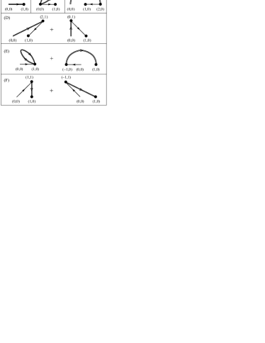
Figure 1: All possible contributions to the photoconductivity at minimal order ${\cal O}(E_{dc}E_{\omega}^{2})$ are illustrated as graphs in $(\nu,n)$ space of angular and temporal harmonics of the distribution function $F_{\nu n}$, according to Eqs. (3.4) and (3.8). The arrows denote coupling of the harmonics $F_{\nu n}$ by the impurity collision integral ${\rm St}_{\rm im}$ [Eq. (2.10)]. The filled circles denote the action of the propagator ${\cal{\cal L}}^{-1}$ in the resulting state. More precisely, ${\rm St}_{\rm im}^{(j,1,2)}$ (which is of third order in the electric fields) is denoted by the thick line in diagram (A), while the first-order collision integrals ${\rm St}_{\rm im}^{(j,1,0)}$ and ${\rm St}_{\rm im}^{(j,0,1)}$ in diagrams (B)–(F) are denoted by the thin lines. The double-line arrows in diagrams (B)–(F) correspond to the second-order integrals ${\rm St}_{\rm im}^{(\bot,1,1)}$ and ${\rm St}_{\rm im}^{(\bot,0,2)}$.

III.2.1 Displacement mechanism (A)

The displacement contribution to the distribution function is obtained by expanding $\hat{{\cal K}}_{j}$ to order ${\cal O}(E_{\rm dc}E_{\omega}^{2})$,

$$\hat{\cal K}^{(1,2)}_{j}=-{6i\over(\tau_{\rm q}\tau_{\rm tr})^{1/2}}(\partial_{\varphi}{\cal X}_{\rm dc}{\cal X}_{\omega}^{2}+{\cal X}_{\rm dc}{\cal X}_{\omega}^{2}\partial_{\varphi})~{},$$ (3.11)

and averaging ${\cal X}_{\omega}^{2}$ over $t$,

$$\overline{{\cal X}_{\omega}^{2}}={1\over 2}({\cal E}_{+}^{2}+{\cal E}_{-}^{2}+2{\cal E}_{+}{\cal E}_{-}\cos 2\varphi)\,\sin^{2}\frac{\omega t_{-}}{2}~{},$$ (3.12)

while neglecting all effects related to $\hat{{\cal K}}_{\bot}$ by putting $\nu=n=0$ in Eq. (3.8). The result,

$$F^{(A)}_{10}=\left<\,e^{-i\varphi}(\omega_{c}\partial_{\varphi})^{-1}\,\overline{{\rm St}_{\rm im}^{(j,1,2)}\{f_{T}\}}\,\right>~{},$$ (3.13)

is represented in Fig. 1 by diagram (A). The thick arrow denotes the action of the term in $\hat{\cal K}^{(1,2)}_{j}$ proportional to $\exp(i\varphi)$, which couples the zero angular harmonic $f_{00}=f_{T}$ to $f_{10}$. The filled circle stands for the propagator ${\cal L}^{-1}=(\omega_{c}\partial_{\varphi})^{-1}$ in the resulting state (1,0).

Equation (3.13) can be understood as follows. In the absence of the microwave field, the dc current occurs due to a difference in the rates of disorder-induced scattering with electron displacements along and against the applied dc field, so that the distribution function becomes anisotropic, Eq. (3.9). Absorption or emission of microwave quanta during these scattering processes, Eq. (3.13), modifies the current by changing the final states and their occupancy. The displacement mechanism of the OPC was predicted long ago in Ref. ryzhii, and addressed in the majority of theoretical worksryzhii ; durst03 ; VA ; shi ; ryzhii03 ; leiliu03 ; park ; lee ; Lyapilin1 ; ryzhii04 ; torres05 ; leiliu05 ; Volkov ; torres06 ; Kashuba06 ; Lyapilin2 ; leiliumulti ; leiliubichrom on the OPC. Its comprehensive study is presented in Ref. VA, .

III.2.2 Inelastic mechanism (B)

The inelastic contribution to the photoconductivity is governed by a change of the isotropic time–independent part of the distribution function, $F_{00}$, due to the absorption and emission of microwave quanta. The change of $F_{00}$ is related to the $t$ and $\varphi$ independent part of the kernel, which, at order ${\cal O}(E_{\omega}^{2})$, is given by

$$\langle\overline{{\cal K}^{(0,2)}_{\bot}}\rangle = -{1\over\tau_{\rm q}}\left<\overline{{\cal X}_{\omega}^{2}}\right>$$ (3.14)

$$= -\frac{1}{2\tau_{\rm q}}({\cal E}_{+}^{2}+{\cal E}_{-}^{2})\,\sin^{2}\frac{\omega t_{-}}{2}~{}.$$

The QBE for $F_{00}$ to order ${\cal O}(E_{\omega}^{2})$ reads

$${\rm St}^{(e-ph)}_{\rm in}\{F_{00}\}+{\rm St}^{(e-e)}_{\rm in}\{F_{00}\}=-\left<\,\overline{{\rm St}_{\rm im}^{(\bot,0,2)}\{f_{T}\}}\,\right>~{}.$$

(3.15)

Equation (3.15) with Eq. (3.14) substituted into the r.h.s. describes two effects: (i) electron heating, i.e., a modification of the smooth part of the electron distribution, and (ii) the appearance of an oscillatory correction to the isotropic part of the distribution on top of the smooth part [cf. Eq. (3.3)]. The heating is controlled by electron–phonon scattering [the first term on the l.h.s. of Eq. (3.15)] and leads to an effective electronic temperature $T_{e}$ larger than the bath temperature $T$. We relegate the discussion of $T_{e}$ as a function of the system parameters and the microwave power to Sec. VIII. Much faster processes of electron-electron inelastic scattering (the second term on the l.h.s.) cannot stabilize the increase of $T_{e}$, but are capable of equilibrating electrons among themselves. The amplitude of the part of $\cal F$ oscillating with $\varepsilon$ in Eq. (3.3) and the amplitude of the oscillations in the photoconductivity are thus proportional to the rate of e–e collisions,long $\tau_{\rm in}^{-1}=\tau_{\rm in}^{-1}(T_{e})$,

$${\rm St}^{(e-e)}_{\rm in}\{F_{00}\}=-\tau_{\rm in}^{-1}F_{00}~{}.$$ (3.16)

Having obtained the nonequilibrium $F_{00}$, we use $\hat{{\cal K}}_{j}$ given by Eq. (3.10) to calculate the linear response with respect to the dc field, so that altogether at order ${\cal O}(E_{\rm dc}E_{\omega}^{2})$ we have:

$$F^{(B)}_{10}=\left<\,e^{-i\varphi}(\omega_{c}\partial_{\varphi})^{-1}{\rm St}_{\rm im}^{(j,1,0)}\left[\tau_{\rm in}\left<\,\overline{{\rm St}_{\rm im}^{(\bot,0,2)}\{f_{T}\}}\,\right>\,\right]\,\right>~{}.$$ (3.17)

Equation (3.17) is represented by diagram (B) in Fig. 1, where the double–line loop denotes the action of $\langle\,\overline{{\rm St}_{\rm im}^{(\bot,0,2)}}\,\rangle$ on $f_{T}$ and the thin arrow corresponds to the action of ${\rm St}_{\rm im}^{(j,1,0)}$ on the resulting $F_{00}$.

One can see that, as compared to the displacement contribution to the OPC, the effect of the inelastic mechanism is accumulated during a much longer time $\tau_{\rm in}\gg\tau_{\rm q}$. The period and the phase of the oscillations are the same for the two mechanisms (and correspond to those observed in the experiment); however, the amplitude of the inelastic contribution is $\tau_{\rm in}/\tau_{\rm q}\gg 1$ times larger. Another important difference is that the $T$ dependence of $\tau_{\rm in}$ makes it possible to explain the temperature-induced decay of the oscillations as observed in the experiment, in contrast to the oscillations produced by the displacement mechanism, which are $T$ independent. The inelastic mechanism of the OPC was proposed in Ref. dmitriev03, and discussed in detail in Ref. long, .

While mechanisms (A) and (B) are widely discussed in the literature, already at first order in the microwave power there exist additional contributions (C)–(F) to the OPC, which have not been studied before.

III.2.3 Quadrupole mechanism (C)

In addition to the effect on $F_{00}$, the absorption and emission of microwave quanta, described by $\hat{{\cal K}}^{(0,2)}_{\bot}=-\tau_{\rm q}^{-1}{\cal X}_{\omega}^{2}$, leads to the appearance of a quadrupole correction $F_{20}$ to the distribution function [see Eq. (3.12)]:

$$F_{20}=\left<e^{-2i\varphi}(\omega_{c}\partial_{\varphi})^{-1}\,\overline{{\rm St}_{\rm im}^{(\bot,0,2)}\{f_{T}\}}\right>~{}.$$ (3.18)

Acting by the operator $\hat{{\cal K}}^{(1,0)}_{j}$ [Eq. (3.10)] on the quadrupole correction yields

$$F^{(C)}_{10}=\left<\,e^{-i\varphi}(\omega_{c}\partial_{\varphi})^{-1}\,{\rm St}_{\rm im}^{(j,1,0)}\{e^{2i\varphi}F_{20}\}\,\right>~{},$$ (3.19)

as illustrated by diagram (C) in Fig. 1.

III.2.4 Photovoltaic mechanism (D)

The photovoltaic contribution to the photoconductivity is generated by the action of

$$\hat{{\cal K}}^{(1,1)}_{\bot}=-2\tau_{\rm q}^{-1}{\cal X}_{\omega}{\cal X}_{dc}$$ (3.20)

on the equilibrium distribution, which leads to the excitation of the components $F_{01}$ and $F_{21}$ oscillating with time. Acting then by

$$\hat{{\cal K}}^{(0,1)}_{j}=-i(\tau_{\rm q}\tau_{\rm tr})^{-1/2}(\partial_{\varphi}{\cal X}_{\omega}+{\cal X}_{\omega}\partial_{\varphi})~{},$$ (3.21)

we calculate the ac response in the resulting state, which gives

$$F^{(D)}_{10} = \left<\,e^{-i\varphi}(\omega_{c}\partial_{\varphi})^{-1}\right.$$

$$\times \left.\overline{{\rm St}_{\rm im}^{(j,0,1)}\left[\,(\omega_{c}\partial_{\varphi}+\partial_{t})^{-1}\,{\rm St}_{\rm im}^{(\bot,\,1,1)}\{f_{T}\}\,\right]}\,\right>~{},$$

see diagrams (D) in Fig. 1

III.2.5 “Inverse-order” contributions (E) and (F)

Additionally, contributions similar to (B)–(D) but with the inverse order of the operators ${\rm St}_{\rm im}^{(j)}$ and ${\rm St}_{\rm im}^{(\bot)}$ in Eq. (3.8) are also possible. Diagrams (E) and (F) in Fig. 1, which describe these processes, involve harmonics of the distribution function different from those in diagrams (B)–(D). Namely, while contributions (B)–(D) include even angular harmonics only, except for the final $F_{10}$, all harmonics in diagrams (E) and (F) are odd in the angle of the momentum, except for the initial $F_{00}=f_{T}$. Despite yielding nonzero contributions to $F_{10}$, diagrams (E) and (F) vanish in the dc current in the limit of high $T$ and strongly overlapping Landau levels [see the paragraph following Eq. (4.11)]. The explicit calculation in Secs. IV and V shows that, in the limit of strongly overlapping Landau levels, mechanisms (A)–(D) give a complete set of contributions to the photoresponse to leading order in the microwave power.

IV QBE for overlapping Landau levels

From now on, we study the effect of microwave radiation on dc transport in the case when the Landau quantization modulates the DOS only weakly. In this limit, the modulation is represented by a single cosine term,

$$\tilde{\nu}(\varepsilon)=\nu(\varepsilon)/\nu_{0}=1-2\delta\,\cos\varepsilon t_{B}~{},\;t_{B}=2\pi/|\omega_{c}|~{},$$ (4.1)

where

$$\delta=\exp(-t_{B}/2\tau_{\rm q})\ll 1~{}.$$ (4.2)

It is worth mentioning that the modulation of the DOS at order ${\cal O}(\delta)$ is insensitive to the external electric fields [correctionsVA ; separated to the DOS induced by the electric fields appear at order ${\cal O}(\delta^{2})$].

The existence of the small parameter $\delta$ greatly simplifies the solution of the kinetic equation in energy space, see Appendix B. The solution can be represented in the form (3.3) with

$${\cal F}(\varepsilon,t,\varphi) = \phi_{0}(\varphi,\,t)$$ (4.3)

$$- 2\delta\;{\rm Re}\,\left[\,\phi_{1}(\varphi,\,t)\exp(i\varepsilon t_{B})\,\right]~{}.$$

For $T\gg t_{B}^{-1}$, the integration over $\varepsilon$ in Eq. (3.4) averages out terms in the current of first order in $\delta$. As a result, in the high-$T$ limit the oscillations of the DOS manifest themselves in the current at order ${\cal O}(\delta^{2})$. We therefore expand $\phi_{0}$ up to a term quadratic in $\delta$:

$$\phi_{0}=\phi_{0}^{\rm D}+2\delta^{2}\phi_{0}^{(2)}~{},$$ (4.4)

where $\phi_{0}^{\rm D}$ is the Drude part independent of $\delta$, and write the current to order ${\cal O}(\delta^{2})$ as

$$\overline{{\bf j}_{d}}=2ev_{F}\nu_{0}{{\rm Re}\choose-{\rm Im}}\left<\,e^{-i\varphi}\,(\,\overline{\phi_{0}}+2\delta^{2}\,{\rm Re}\,\overline{\phi_{1}}\,)\,\right>~{}.$$ (4.5)

It is convenient to introduce new functions $\phi_{j}$ and $\phi_{\bot}$ according to

$$\phi_{j}=\phi_{0}^{(2)}+{\rm Re}\,\phi_{1}\,,$$ (4.6)

$$\phi_{\bot}={\rm Im}\,\phi_{1}~{},$$ (4.7)

after which the current (4.5) is split into the classical (Drude) and quantum parts as follows:

$$\overline{{\bf j}_{d}}=2\sigma_{xx}^{\rm D}{\bf E}_{\rm dc}+4\delta^{2}ev_{F}\nu_{0}{{\rm Re}\choose{\rm Im}}\left\langle\,e^{i\varphi}\,\overline{\phi_{j}}\,\right\rangle~{}.$$ (4.8)

As shown in Appendix B, the functions $\phi_{0}^{\rm D}$, $\phi_{j}$, and $\phi_{\bot}$ obey

$$i(\partial_{t}+\omega_{c}\partial_{\varphi})\phi_{0}^{\rm D}=\partial_{t_{-}}\left.\hat{\cal K}_{j}(t,t_{-})\right|_{t_{-}=0}~{},$$ (4.9)

$$\left.i(\partial_{t}+\omega_{c}\partial_{\varphi})\phi_{j}=(\partial_{t_{-}}-{1\over 2}\partial_{t})\hat{\cal K}_{j}(t,t_{-})\right|_{t_{-}=t_{B}}$$

$$\qquad-\hat{\cal K}_{j}(t,t_{B})\phi_{\bot}-\phi_{\bot}\hat{\cal K}_{j}(t,t_{B})~{},$$ (4.10)

$$[\partial_{t}+\omega_{c}\partial_{\varphi}-\hat{\cal K}_{\bot}(t,t_{B})]\phi_{\bot}+\tau_{\rm in}^{-1}\left\langle\phi_{\bot}\right\rangle$$

$$\left.\qquad=({1\over 2}\partial_{t}-\partial_{t_{-}})\hat{\cal K}_{\bot}(t,t_{-})\right|_{t_{-}=t_{B}}~{}.$$ (4.11)

Here and below, any operator $\hat{{\cal K}}_{j,\bot}$ in the rightmost position is understood as acting on unity.

The first term on the r.h.s. of Eq. (4.10) gives the displacement contribution (A) to the dc current (4.8), while the second and third terms yield the inelastic, quadrupole, and photovoltaic contributions (B)–(D). It is important to notice that Eq. (4.10) for the function $\phi_{j}$ includes the odd part of the kernel $\hat{\cal K}_{j}$ only, while the function $\phi_{\bot}$ [Eq. (4.11)] is completely determined by the even part $\hat{\cal K}_{\bot}$. It follows that diagrams (E) and (F) in Fig. 1 produce no contribution to the dc current, because of the absence of coupling between $\phi_{j}$ and $\hat{\cal K}_{\bot}$. Although the functions $\phi_{0}^{(2)}$ and ${\rm Re}\phi_{1}$ are coupled with each other [see Eqs. (B.6) and (B.8)] and do have contributions of type (E) and (F), each of these contributions vanishes in the combination $\phi_{j}$ [Eq. (4.6)] which determines the current according to Eq. (4.8).

As follows from Eq. (4.8), for the calculation of $\overline{{\bf j}_{d}}$ we need only the $t$ independent parts of $\phi_{0}^{\rm D}$ and $\phi_{j}$. Using the explicit form of $\hat{{\cal K}}_{j}$ [Eq. (LABEL:Kj)] and the fact that ${\cal X}(t_{-}=0)=0$, the r.h.s. of Eq. (4.9) averaged over $t$ reads

$$\partial_{t_{-}}\!\left.\overline{\hat{\cal K}_{j}(t,t_{-})}\right|_{t_{-}=0}=-i\partial_{\varphi}\frac{\partial_{t_{-}}{\cal X}_{\rm dc}}{\sqrt{\tau_{\rm q}\tau_{\rm tr}}}~{},$$ (4.12)

which gives

$$\overline{\phi_{0}^{\rm D}}=\frac{ev_{F}}{\omega_{c}^{2}\tau_{\rm tr}}{\bf E}_{\rm dc}{\cos\varphi\choose\sin\varphi}$$ (4.13)

and, correspondingly, the Drude conductivity

$$\sigma_{xx}^{\rm D}=\frac{e^{2}\nu_{0}v_{F}^{2}}{2\omega_{c}^{2}\tau_{\rm tr}}~{}.$$ (4.14)

Similarly,

$$\overline{\phi_{j}}=\overline{\frac{-\partial_{t_{B}}+2\phi_{\bot}}{\omega_{c}\sqrt{\tau_{\rm q}\tau_{\rm tr}}}\,\frac{X}{(1+X^{2})^{2}}}~{},$$ (4.15)

where

$$X\equiv{\cal X}|_{t_{-}=t_{B}}=X_{\rm dc}+X_{\omega}$$ (4.16)

and for later use we introduce also

$$X_{\omega} \equiv \left.{\cal X}_{\omega}\right|_{t_{-}=t_{B}}~{},$$

$$X_{\rm dc} \equiv \left.{\cal X}_{\rm dc}\right|_{t_{-}=t_{B}}~{}.$$ (4.17)

The derivative $\partial_{t_{B}}$ in Eq. (4.15) should be understood according to the notation which we also use below in the paper:

$$\partial_{t_{B}}A(X_{\omega},X_{\rm dc})\equiv\partial_{t_{-}}A({\cal X}_{\omega},{\cal X}_{\rm dc})|_{t_{-}=t_{B}}~{},$$ (4.18)

where $A$ is an arbitrary function.

Now that $\overline{\phi_{j}}$, which determines the dc current (4.8), is obtained in the form of Eq. (4.15), the problem of finding the OPC to arbitrary order in $E_{\omega}^{2}$ or $E_{\rm dc}$ is reduced to solving Eq. (4.11) for the function $\phi_{\bot}$. In this paper, we restrict ourselves to the calculation of the linear response with respect to the dc field. In Sec. V, we obtain explicit expressions for the linear photoconductivity, corresponding to $\overline{\bf j}\propto E_{\rm dc}E_{\omega}^{2}$. With increasing microwave power, the system passes through several nonlinear regimes, which are studied in Secs. VI, VII, and VIII.

V Linear photoconductivity

According to the general classification presented in Sec. III, at order ${\cal O}(E_{\rm dc}E_{\omega}^{2})$ one can distinguish four different mechanisms of the photoconductivity, illustrated by diagrams (A)–(D) in Fig. 1. We now calculate terms in the photoconductivity associated with the corresponding nonequilibrium corrections to the distribution function, given by Eqs. (3.8), (3.13), (3.17), (3.19), and (LABEL:fD).

The displacement contribution (A), Eq. (3.13), is produced by ${\cal K}^{(1,2)}_{j}\propto E_{\rm dc}E_{\omega}^{2}$. All effects on even angular harmonics of the distribution function, governed by $\hat{{\cal K}}_{\bot}$, are neglected, i.e., $\phi_{\bot}^{(A)}=0$. Equation (4.15) then reduces to

$$\overline{\phi_{j}^{(A)}}=\frac{6\,\partial_{t_{B}}}{\omega_{c}\sqrt{\tau_{\rm q}\tau_{\rm tr}}}\,X_{\rm dc}\overline{X_{\omega}^{2}}~{}.$$ (5.1)

By contrast, contributions (B)–(D) are related to the effect of the microwave and dc fields on even angular harmonics. At order ${\cal O}(X^{2})$, Eq. (4.11) reads

$$(\partial_{t}+\omega_{c}\partial_{\varphi})\phi_{\bot}+\tau_{\rm in}^{-1}\left\langle\phi_{\bot}\right\rangle=\tau_{\rm q}^{-1}(\partial_{t_{B}}-\partial_{t}/2)X^{2}~{}.$$ (5.2)

To linear order in the dc field, we replace $X^{2}$ in the r.h.s. of Eq. (5.2) by $X_{\omega}^{2}+2X_{\omega}X_{\rm dc}$. The isotropic and quadrupole parts of $\overline{X_{\omega}^{2}}$ [Eq. (3.12)] yield the inelastic (B) and quadrupole (C) contributions, respectively, while the photovoltaic contribution (D) is generated by the product $X_{\omega}X_{\rm dc}$:

$$\phi_{\bot}^{(B)}=\frac{\tau_{\rm in}}{\tau_{\rm q}}\partial_{t_{B}}\langle\overline{X_{\omega}^{2}}\rangle~{},$$ (5.3)

$$\phi_{\bot}^{(C)}=\frac{\partial_{t_{B}}}{\omega_{c}\tau_{\rm q}\partial_{\varphi}}\left(\overline{X_{\omega}^{2}}-\langle\overline{X_{\omega}^{2}}\rangle\right)~{},$$ (5.4)

$$\phi_{\bot}^{(D)}=\tau_{\rm q}^{-1}(\partial_{t}+\omega_{c}\partial_{\varphi})^{-1}(2\partial_{t_{B}}-\partial_{t})X_{\omega}X_{\rm dc}~{}.$$

(5.5)

In Eqs. (5.3)–(5.5), $\phi_{\bot}^{(B)}$ and $\phi_{\bot}^{(C)}$ are averaged over $t$, whereas $\phi_{\bot}^{(D)}$ is not. The current (4.8) is then produced by the dc [in the case of (B) and (C)] or ac [in the case of (D)] response in the resulting state:

$$\overline{\phi_{j}}=\frac{2}{\omega_{c}\sqrt{\tau_{\rm q}\tau_{\rm tr}}}\,\overline{\phi_{\bot}(X_{\rm dc}+X_{\omega})}~{}.$$ (5.6)

Substituting Eqs. (5.3)–(5.5) into Eq. (5.6) and using the resulting $\overline{\phi_{j}}$ together with $\overline{\phi_{j}^{(A)}}$ [Eq. (5.1)] in Eq. (4.8) yields the current ${\bf\overline{j}}=\hat{\sigma}_{\rm ph}{\bf E}_{\rm dc}$.

It is convenient to parametrize the photoconductivity tensor $\hat{\sigma}_{\rm ph}$ by four functions $d_{s}$, $d_{a}$, $h_{s}$, $h_{a}$:

$$\frac{\hat{\sigma}_{\rm ph}}{2\sigma^{\rm D}_{xx}} = \left(\!\begin{array}[]{cc}1+2\delta^{2}&-\omega_{c}\tau_{\rm tr}\\ \omega_{c}\tau_{\rm tr}&1+2\delta^{2}\end{array}\!\right)$$ (5.9)

$$- 2\delta^{2}\left(\!\begin{array}[]{cc}d_{s}&h_{a}\\ -h_{a}&d_{s}\end{array}\!\right)-2\delta^{2}\left(\!\begin{array}[]{cc}d_{a}&h_{s}\\ h_{s}&-d_{a}\end{array}\!\right)~{}.$$ (5.14)

The first matrix in Eq. (LABEL:sigmaph1) is the linear dc conductivity in the absence of microwaves. The quantum correction $2\delta^{2}$ to the dissipative part comes from inserting Eq. (4.15) into Eq. (4.8) if one puts $\phi_{\bot}=0$ in Eq. (4.15) and also substitute $X_{\rm dc}$ for $X/(1+X^{2})^{2}$. The resulting $\overline{\phi_{j}}$ coincides with $\phi_{0}^{\rm D}$ [Eq. (4.13)].

Two other matrices in Eq. (LABEL:sigmaph1) represent the microwave–induced corrections. We express the elements of these matrices in terms of the following dimensionless parameters:

$$w = \omega t_{B}/2=\pi\omega/|\omega_{c}|~{},$$ (5.16)

$$Q = \sin^{2}w\,({\cal E}_{+}^{2}+{\cal E}_{-}^{2})~{},$$ (5.17)

$$Q_{\rm AI} = \sin^{2}w\,{\cal E}_{+}{\cal E}_{-}~{},$$ (5.18)

$$Q_{\rm S} = 2\sin^{2}w$$ (5.19)

$$\times \left({\cal E}_{+}^{2}\,\frac{\omega+\omega_{c}}{\omega+2\omega_{c}}+{\cal E}_{-}^{2}\,\frac{\omega-\omega_{c}}{\omega-2\omega_{c}}\right)~{},$$

$$Q_{\rm AS} = 2\sin^{2}w\,{\omega_{c}^{2}\over\omega}$$ (5.20)

$$\times \left({\cal E}_{+}^{2}\,\frac{1}{\omega+2\omega_{c}}+{\cal E}_{-}^{2}\,\frac{1}{\omega-2\omega_{c}}\right)~{},$$

where ${\cal E}_{\pm}$ are defined in Eq. (2.24). In addition to the effective microwave power $Q$ we introduced three similar parameters, Eqs. (5.18)-(5.20), with the subscripts “AI”,“S”, and “AS” standing for “anisotropic”, “symmetric”, and “antisymmetric”, respectively (in accord with their appearance in the corresponding components of $\hat{\sigma}_{\rm ph}$, see below).

The diagonal isotropic part $d_{s}$ of $\hat{\sigma}_{\rm ph}$, Eq. (LABEL:sigmaph1), is a sum of the displacement, inelastic, and photovoltaic contributions:

$$d_{s} = d_{s}^{(A)}+d_{s}^{(B)}+d_{s}^{(D)}~{},$$ (5.21)

$$d_{s}^{(A)} = 3Q+6Q\,w\cot w~{},$$ (5.22)

$$d_{s}^{(B)} = 2{\tau_{\rm in}\over\tau_{\rm q}}Q\,w\cot w~{},$$ (5.23)

$$d_{s}^{(D)} = -{w\,Q_{\rm S}\over\omega\tau_{\rm q}}~{}.$$ (5.24)

The diagonal anisotropic part $d_{a}$ is governed by the displacement and photovoltaic mechanisms:

$$d_{a} = d_{a}^{(A)}+d_{a}^{(D)}~{},$$ (5.25)

$$d_{a}^{(A)} = 6Q_{\rm AI}(1+2w\cot w)~{},$$ (5.26)

$$d_{a}^{(D)} = -{4w\,Q_{\rm AI}\over\omega\tau_{\rm q}}~{}.$$ (5.27)

The nondiagonal symmetric term $h_{s}$ is due to the quadrupole mechanism:

$$h_{s}=h_{s}^{(C)}={Q_{\rm AI}\over\omega_{c}\tau_{\rm q}}\,w\cot w~{},$$ (5.28)

while the antisymmetric Hall part is generated by the photovoltaic mechanism:

$$h_{a}=h_{a}^{(D)}={Q_{\rm AS}\over\omega_{c}\tau_{\rm q}}(1+w\cot w)~{}.$$ (5.29)

Let us now discuss the results (5.21)–(5.29), obtained for the linear regime in the microwave power:

• the inelastic mechanism yields the dominant effect because of $\tau_{\rm in}/\tau_{\rm q}\gg 1$: ${\rm(B)\gg(A),(C),(D)}$;

• ${\rm(C),(D)\gg(A)}$ for the case of $\omega_{c}\tau_{\rm q}\sim\omega\tau_{\rm q}\ll 1$ (strongly overlapping Landau levels). Note, however, that since $\delta$ [Eq. (4.2)] depends exponentially on $\omega_{c}$, a pronounced effect (from the practical point of view) is only possible at not too small magnetic fields. The effects of (A), (C), and (D) are then comparable in magnitude, differing only in $\ln\delta$;

• although ${\rm(B)\gg(C),(D)}$, the oscillatory corrections to the Hall conductivity are entirely governed by the quadrupole (C) and photovoltaic (D) mechanisms;

• the quadrupole contribution $h_{s}$ violates Onsager symmetry: $\sigma_{ik}(B,s_{-},s_{+})\neq\sigma_{ki}(-B,s_{+},s_{-})$ [the effect of time inversion on the microwave field polarization can be expressed as $s_{+}\leftrightarrows s_{-}$, which is equivalent to $\omega\to-\omega$, see Eq. (2.24)]. Although Onsager symmetry need not be satisfied in nonequilibrium systems, there exist not many examples of its violation. One of them, for a different system but under similar conditions, was found in Ref. antionsager, . Symmetry with respect to the parity transformation, $x\to-x$, must be satisfied: $\sigma_{ik}(B,s_{-},s_{+})=r_{ik}\sigma_{ik}(-B,s_{+},s_{-})$, where $r_{xx}=r_{yy}=1$, $r_{xy}=r_{yx}=-1$. It can be easily verified in our case since all parameters (5.16)–(5.20) are unaffected by the simultaneous change $B\to-B$ and $s_{+}\leftrightarrows s_{-}$;

• the quadrupole term $h_{s}$ and the anisotropic term in the diagonal photoresponse $d_{a}$ vanish in the case of circular polarization of the microwaves ($Q_{\rm AI}=0$).

VI Feedback effect: Saturation of the inelastic contribution (SIC)

The results for $\hat{\sigma}_{\rm ph}\propto E_{\omega}^{2}$ obtained in Sec. V, are valid at not too high microwave power. The QBE in the form (4.11) contains two sources of nonlinearity in $E_{\omega}^{2}$. At $Q\gtrsim 1$, high-order terms in the expansion of $\hat{{\cal K}}_{j}$ and ${\cal K}_{\bot}$ in powers of $E_{\omega}$ become important, leading to multiphoton corrections to both $\phi_{\bot}$ and $\phi_{j}$, see Eqs. (4.11) and (4.15). The other source of nonlinearity, the “feedback” term ${\cal K}_{\bot}\phi_{\bot}$ in Eq. (4.11), strongly modifies the photoresponse at much smaller microwave power, $Q_{\rm in}\sim 1$, where

$$Q_{\rm in}\equiv\frac{\tau_{\rm in}}{2\tau_{\rm q}}Q~{}.$$ (6.1)

Since $\tau_{\rm in}\gg\tau_{\rm q}$, the multiphoton corrections can still be neglected at $Q_{\rm in}\sim 1$. As we show below in this section, at $Q_{\rm in}\gg 1$ the single–photon feedback effect leads to a saturation of the inelastic contribution and to a strong modification of all other contributions to the photoconductivity.

VI.1 Feedback effect on the isotropic part of the distribution

The feedback effect on the inelastic mechanism was studied in detail in Ref. long, . Here, we reproduce the resultslong within the more general framework of Secs. III and IV. Using Eq. (2.26), we rewrite Eq. (4.11) in the limit $Q\ll 1$ as

$$\left(\partial_{t}+\omega_{c}\partial_{\varphi}+\frac{X^{2}}{\tau_{\rm q}}\right)\phi_{\bot}+\frac{\langle\phi_{\bot}\rangle}{\tau_{\rm in}}=\frac{2\partial_{t_{B}}-\partial_{t}}{2\tau_{\rm q}}X^{2}~{}.$$ (6.2)

Averaging Eq. (6.2) over $t$ and $\phi$, we obtain the equation for the isotropic time-independent part $\phi_{\bot}^{(B)}\equiv\langle\overline{\phi_{\bot}}\rangle$:

$$\left(\frac{\tau_{\rm q}}{\tau_{\rm in}}+\left<\overline{X_{\omega}^{2}}\right>\right)\phi_{\bot}^{(B)}$$

$$=\partial_{t_{B}}\left<\overline{X_{\omega}^{2}}\right>-\left<\overline{X_{\omega}^{2}\left(\phi_{\bot}-\phi_{\bot}^{(B)}\right)}\right>~{}.$$ (6.3)

In the linear regime with respect to the microwave power, i.e., for $Q\ll\tau_{\rm q}/\tau_{\rm in}$, we return to $\phi_{\bot}^{(B)}\propto Q$ given by Eq. (5.3). At $Q\sim\tau_{\rm q}/\tau_{\rm in}\ll 1$ two terms on the l.h.s. of Eq. (6.3) become of the same order of magnitude, whereas the last term on the r.h.s. is still small and can be neglected (corrections of higher order in $Q$, generated by this term, are considered in Sec. VI.3). We thus obtain for $Q\ll 1$ and arbitrary order in $Q_{\rm in}$:

$$\phi_{\bot}^{(B)}=\frac{Q_{\rm in}}{1+Q_{\rm in}}\omega\cot w~{}.$$ (6.4)

It follows that in the limit $Q_{\rm in}\gg 1$ we reach a saturation of the inelastic contribution (SIC):

$$\phi_{\bot}^{(B)}\to\frac{\partial_{t_{B}}\langle\overline{X_{\omega}^{2}}\rangle}{\langle\overline{X_{\omega}^{2}}\rangle}=\omega\cot\frac{\pi\omega}{|\omega_{c}|}~{}.$$ (6.5)

The dc response in the stationary nonequilibrium state (6.4) yields

$$d_{s}^{(B)}=\frac{4\,Q_{\rm in}}{1+Q_{\rm in}}\,w\cot w~{},$$ (6.6)

reproducing Eq. (15) of Ref. long, .

The saturation of the inelastic contribution at large $Q_{\rm in}$ has much in common with the well-known effect of “self-induced transparency” for a two-level system in a strong resonant electromagnetic field, which occurs due to equalization of the population of the levels. Clearly, in the system we consider here the complete transparency cannot be obtained since the electron spectrum in our problem is continuous. Even in the SIC regime, absorption does not tend to zero. Electrons still absorb microwave quanta and transmit the absorbed power to the phonon bath: the dynamic equilibrium between these two processes determines the effective electronic temperature $T_{e}$, see Sec. IX. However, the saturation (6.5) of the amplitude of the oscillations in the isotropic part of the distribution function is governed by the same feedback effect as the transparency in the two–level system.

VI.2 Quadrupole, photovoltaic, and displacement contributions in the SIC regime

In the nonlinear regime, the strong oscillations of $F_{00}(\varepsilon)$ produced by the inelastic mechanism essentially modify contributions (A), (C), and (D). Since $\phi_{\bot}^{(C)}$ and $\phi_{\bot}^{(D)}$ are still small at $Q_{\rm in}\sim 1$, we replace $\phi_{\bot}$ in the term $X^{2}\phi_{\bot}/\tau_{\rm q}$ on the l.h.s. of Eq. (6.2) by $\phi_{\bot}^{(B)}$. Solving Eq. (6.2) for the quadrupole and photovoltaic contributions then gives:

$$\phi_{\bot}^{(CB)} = \partial_{\varphi}^{-1}\,{\partial_{t_{B}}-\phi_{\bot}^{(B)}\over\omega_{c}\tau_{\rm q}}\left(\overline{X_{\omega}^{2}}-\langle\overline{X_{\omega}^{2}}\rangle\right)~{},$$ (6.7)

$$\phi_{\bot}^{(DB)} = 2(\partial_{t}+\omega_{c}\partial_{\varphi})^{-1}$$ (6.8)

$$\times \frac{\partial_{t_{B}}-\partial_{t}/2-\phi_{\bot}^{(B)}}{\tau_{\rm q}}\,X_{\omega}X_{\rm dc}~{}.$$

Here and below we emphasize the influence of the inelastic mechanism by adding the second superscript $B$. Substituting Eqs. (6.7) and (6.8) into Eq. (4.15) and using the resulting $\overline{\phi_{j}}$ in Eq. (4.8) yields the photovoltaic and quadrupole contributions to the Hall part of $\hat{\sigma}_{\rm ph}$ [Eq. (LABEL:sigmaph1)]:

$$h_{s}^{(CB)}={Q_{\rm AI}\over\omega_{c}\tau_{\rm q}}\,\frac{w\cot w}{Q_{\rm in}+1}\,,\;\;\;$$ (6.9)

$$h_{a}^{(DB)}={Q_{\rm AS}\over\omega_{c}\tau_{\rm q}}\left(1-\frac{Q_{\rm in}-1}{Q_{\rm in}+1}w\cot w\right)~{}.$$ (6.10)

The diagonal photovoltaic contributions $d_{s}^{(D)}$ and $d_{a}^{(D)}$, which originate from the derivative $\partial_{t}$ in Eq. (6.8), are not affected by the oscillations in $F_{00}$ and remain the same as in the linear regime, Eqs. (5.24) and (5.27).

The oscillations of $F_{00}$ also modify the displacement contribution to the current. Similarly to Eqs. (6.7) and (6.8) we substitute $\phi_{\bot}^{(B)}$ for $\phi_{\bot}$ in Eq. (4.15), which gives

$$\overline{\phi_{j}^{(AB)}}=\frac{\partial_{t_{B}}-2\phi_{\bot}^{(B)}}{\omega_{c}\sqrt{\tau_{\rm q}\tau_{\rm tr}}}\,6X_{\rm dc}\overline{X_{\omega}^{2}}~{}.$$ (6.11)

Using Eq. (6.11) in Eq. (4.8) we have

$$d_{s}^{(AB)}=3Q\left(1-\frac{Q_{\rm in}-1}{Q_{\rm in}+1}\,2w\cot w\right)~{},$$ (6.12)

$$d_{a}^{(AB)}=6Q_{\rm AI}\left(1-\frac{Q_{\rm in}-1}{Q_{\rm in}+1}\,2w\cot w\right)~{}.$$

(6.13)

We thus see that in the SIC regime, $Q_{\rm in}\gg 1$, the quadrupole term $h_{s}^{(CB)}$ saturates as a function of the microwave power, whereas the nondiagonal photovoltaic term $h_{a}^{(DB)}$ and the both displacement terms $d_{s}^{(AB)}$ and $d_{a}^{(AB)}$ continue to grow linearly with increasing power but are strongly modified as compared to the linear regime.

VI.3 Two–photon and double–frequency corrections to the isotropic part of the distribution

For $Q_{\rm in}\gg 1$, the main (inelastic) contribution to the oscillatory part of the photoconductivity is independent of the microwave power as long as $Q$ is sufficiently small. Deviations from the “plateau” come from contributions (A) and (D) (which, as shown in Sec. VI.2, grow linearly with $Q$ in the SIC regime), and also from corrections of order ${\cal O}(Q)$ to the $Q$ independent term $\phi_{\bot}^{(B)}$ [Eq. (6.5)], which we obtain below.

Equation (4.11) produces two types of corrections to $\phi_{\bot}^{(B)}$ of linear order in $Q$. One of them is related to two–photon processes in $\hat{{\cal K}}_{\bot}$, which come from the expansion of ${\cal K}_{\bot}$ to fourth order in ${\cal X}_{\omega}$, yielding

$$\phi_{\bot}^{(B)}=\frac{\partial_{t_{B}}\langle\overline{X_{\omega}^{2}-X_{\omega}^{4}}\rangle}{\tau_{\rm q}\tau_{\rm in}^{-1}+\langle\overline{X_{\omega}^{2}-X_{\omega}^{4}}\rangle}$$

$$=\omega\cot w\,\frac{Q_{\rm in}}{Q_{\rm in}+1}\left(1-{3\over 4}Q\frac{Q_{\rm in}+2}{Q_{\rm in}+1}\right)~{}.$$ (6.14)

The other is associated with single–photon excitation of the second temporal harmonic of the distribution function. This correction originates from the term $\partial_{t}X_{\omega}^{2}$ in Eq. (6.2) (which has played no role so far) and to leading order in $X_{\omega}^{2}$ reads:

$$\phi_{\bot}^{(2\omega)}=C-\frac{(2\tau_{\rm q})^{-1}}{\partial_{t}+\omega_{c}\partial_{\varphi}}\,\partial_{t}\left(X_{\omega}^{2}-\overline{X_{\omega}^{2}}\right)~{},$$ (6.15)

where

$$X_{\omega}^{2}-\overline{X_{\omega}^{2}} = {1\over 2}\sin^{2}w\left[\,{\cal E}_{+}^{2}\cos(2\omega t+2\varphi)\right.$$

$$+ \left.{\cal E}_{-}^{2}\cos(2\omega t-2\varphi)+2{\cal E}_{+}{\cal E}_{-}\cos 2\omega t\,\right]~{}.$$

The constant of integration $C$ in Eq. (6.15) should be found from the periodic boundary condition for the function $\phi_{\bot}^{(2\omega)}(\varphi,t)$. Averaging Eq. (6.2) over $\varphi$ and $t$, we get the boundary condition in the form $\tau_{\rm in}\langle\overline{X_{\omega}^{2}\phi_{\bot}^{(2\omega)}}\rangle=-\tau_{\rm q}\langle\overline{\phi_{\bot}^{(2\omega)}}\rangle$, which gives $C=\tau_{\rm q}^{-1}Q_{2\omega}Q_{\rm in}/(1+Q_{\rm in})$, where

$$Q_{2\omega}=\frac{\sin^{4}w}{8Q}\left(4{\cal E}_{+}^{2}{\cal E}_{-}^{2}+\frac{\omega}{\omega+\omega_{c}}{\cal E}_{+}^{4}+\frac{\omega}{\omega-\omega_{c}}{\cal E}_{-}^{4}\right)~{}.$$

(6.17)

Only the constant $C$ contributes to the double-frequency correction to the dc current at first order in $Q$. Summing up the contributions (6.14) and (6.15) to $\phi_{\bot}^{(B)}$ we obtain $d_{s}^{(B)}=2t_{B}\phi_{\bot}^{(B)}$ with the linear-in-$Q$ terms included:

$$d_{s}^{(B)}\simeq\frac{4w\,Q_{\rm in}}{1+Q_{\rm in}}\,\left[\,\cot w\left(1-{3\over 4}Q\,\frac{Q_{\rm in}+2}{Q_{\rm in}+1}\right)+\frac{Q_{2\omega}}{\omega\tau_{\rm q}}\,\right]~{}.$$

(6.18)

Equation (6.18) tells us that for strongly overlapping Landau levels the double-frequency correction is much stronger than the one coming from the two-photon processes, except for the close vicinity of the cyclotron-resonance harmonics where the two-photon correction exhibits singular behavior.

VI.4 Discussion of the results

Equations (6.9), (6.10), (6.12), (6.13), and (6.18), together with Eqs. (5.24) and (5.27), describe the photoconductivity $\hat{\sigma}_{\rm ph}$ [Eq. (LABEL:sigmaph1)] to arbitrary order in $Q_{\rm in}=\tau_{\rm in}Q/2\tau_{\rm q}$ and to first order in $Q$. In the limit $Q_{\rm in}\ll 1$, Eqs. (5.21)–(5.29) are reproduced. At $Q_{\rm in}\gtrsim 1$, the evolution of the photoresponse with increasing power can be summarized as following:

• Growth of the leading (inelastic) term $d_{s}^{(B)}$ saturates due to the feedback effect, Eq. (6.6), and so does the quadrupole term $h_{s}^{(CB)}$, Eq. (6.9).

• Remarkably, the parts proportional to $w\cot w$ of the displacement contributions $d_{s}^{(AB)}$ and $d_{a}^{(AB)}$, as well as that of the photovoltaic contribution $h_{a}^{(DB)}$, change sign at $Q_{\rm in}=1$, and the linear growth is recovered with opposite sign at higher power.

• While at $Q_{\rm in}\ll 1$ the inelastic contribution is the only one that is $T$ dependent, in the crossover region, $Q_{\rm in}\sim 1$, all contributions, except for the diagonal photovoltaic terms $d_{s}^{(D)}$ and $d_{a}^{(D)}$, change strongly as a function of $T$.

• However, apart from the small quadrupole correction $h_{s}^{(CB)}$, the photoconductivity in the limit $Q_{\rm in}\gg 1$ becomes independent of $\tau_{\rm in}$ and, hence, of temperature:

$$d_{s}^{(B)} = w\cot w(4-3Q)+4wQ_{2\omega}/\omega\tau_{\rm q}~{},$$ (6.19)

$$d_{s}^{(AB)} = 3Q\left(1-2w\cot w\right)~{},$$ (6.20)

$$d_{a}^{(AB)} = 6Q_{\rm AI}(1-\,2w\cot w)~{},$$ (6.21)

$$d_{s}^{(D)} = w\,Q_{\rm S}/\omega\tau_{\rm q}~{},$$ (6.22)

$$d_{a}^{(D)} = -4w\,Q_{\rm AI}/\omega\tau_{\rm q}~{},$$ (6.23)

$$h_{s}^{(CB)} = (Q_{\rm AI}/Q_{\rm in})w\cot w/\omega_{c}\tau_{\rm q}~{},$$ (6.24)

$$h_{a}^{(DB)} = Q_{\rm AS}(1-w\cot w)/\omega_{c}\tau_{\rm q}~{}.$$ (6.25)

Equations (6.19)–(6.25) predict that there are two sources of nonlinearities which will essentially modify the plateau behavior in the SIC regime with increasing microwave power: the multiphoton processes and the “spreading” of the feedback effect over higher temporal and angular harmonics. The multiphoton effects become strong at $Q\gtrsim 1$, whereas the feedback-related excitation of distant harmonics becomes strong already at much lower power, namely at $Q\gtrsim\omega_{c}\tau_{\rm q}$. It is important that the strong deviations from the plateau behavior take place when $Q$ is already much larger than $\tau_{\rm q}/\tau_{\rm in}$ and, therefore, inelastic scattering can be completely neglected. In Sec. VII we discuss the regime of ultrahigh power in more detail.

VII Ultrahigh power: Feedback vs multiphoton effects

VII.1 Classification of contributions to $\hat{\sigma}_{\rm ph}$ at ultrahigh power

In the SIC regime considered in Sec. VI, strong oscillations in isotropic part of the distribution function essentially modified all contributions to the dc current (A)–(D). At ultrahigh power, contributions involving high angular and temporal harmonics of the distribution function become important, so that our previous (A)–(D) classification, developed in Sec. III for the linear $\hat{\sigma}_{\rm ph}$, should be generalized. Despite the excitation of the high harmonics, at ultrahigh power it is still possible to distinguish the generalized displacement (A), photovoltaic (D), and non-photovoltaic contributions. In the linear regime with respect to the dc field $E_{\rm dc}$, the latter enters the part of the kernel $\hat{\cal K}_{\bot}$ in the photovoltaic term only. In all other terms, $E_{\rm dc}$ belongs to $\hat{\cal K}_{j}$. Further, in the displacement term all effects of the microwave and dc fields on even angular harmonics are absent. We now proceed to calculate various contributions to $\hat{\sigma}_{\rm ph}$ in the limit of ultrahigh power, where the inelastic scattering is of no importance.

The displacement contribution is readily calculated to arbitrary order in microwave power by putting $\phi_{\bot}=0$ in Eq. (4.15) for $\phi_{j}$ and extracting the part linear in $E_{\rm dc}$:

$$\phi_{j}^{(A)} = \frac{ev_{F}}{\omega_{c}^{2}\tau_{\rm tr}}\,{\rm Re}\,\left(E_{\rm dc}^{+}\,e^{-i\varphi}\right)$$ (7.1)

$$\times \partial_{t_{B}}t_{B}\frac{1-3X_{\omega}^{2}}{(1+X_{\omega}^{2})^{3}}~{},$$

where $E_{\rm dc}^{+}=({\bf E}_{\rm dc})_{x}+i({\bf E}_{\rm dc})_{y}$ and we used the explicit form of $X_{\rm dc}$ given by Eq. (2.22). As for the effect of the ac and dc fields on even angular harmonics, Eq. (4.15) yields:

$$\phi_{j}^{(0)}=\frac{2\phi_{\bot}^{(0)}X_{\rm dc}}{\omega_{c}\sqrt{\tau_{\rm q}\tau_{\rm tr}}}\,\frac{1-3X_{\omega}^{2}}{(1+X_{\omega}^{2})^{3}}~{},$$ (7.2)

$$\phi_{j}^{(D)}=\frac{2\phi_{\bot}^{(D)}}{\omega_{c}\sqrt{\tau_{\rm q}\tau_{\rm tr}}}\,\frac{X_{\omega}}{(1+X_{\omega}^{2})^{2}}~{}.$$ (7.3)

Here $\phi_{\bot}^{(0)}$ is the solution of Eq. (4.11) that is independent of $E_{\rm dc}$ (at small power, $\phi_{\bot}^{(0)}$ is the sum of the inelastic and quadrupole terms) and $\phi_{\bot}^{(D)}$ is the linear-in-$E_{\rm dc}$ (photovoltaic) solution:

$$\left(\partial_{t}+\omega_{c}\partial_{\varphi}+{1\over\tau_{\rm q}}\frac{X_{\omega}^{2}}{1+X_{\omega}^{2}}\right)\phi_{\bot}^{(0)}$$

$$\quad=\frac{\partial_{t_{B}}-\partial_{t}/2}{\tau_{\rm q}}\frac{X_{\omega}^{2}}{1+X_{\omega}^{2}}~{},$$ (7.4)

$$\left(\partial_{t}+\omega_{c}\partial_{\varphi}+{1\over\tau_{\rm q}}\frac{X_{\omega}^{2}}{1+X_{\omega}^{2}}\right)\phi_{\bot}^{(D)}$$

$$\quad=\frac{\partial_{t_{B}}-\partial_{t}/2-\phi_{\bot}^{(0)}}{\tau_{\rm q}}\,\frac{2X_{\rm dc}X_{\omega}}{(1+X_{\omega}^{2})^{2}}~{}.$$ (7.5)

In Eq. (7.4), we omitted the term which describes inelastic scattering, since in the following we consider the limit $Q\gg\tau_{\rm q}/\tau_{\rm in}$. In this limit, the inelastic scattering is irrelevant, as demonstrated in Sec. VI.4. For simplicity, we focus here on the case of circularly polarized microwaves. Linear polarization is briefly discussed in the end of Sec. VII.3.

VII.2 Circular polarization: General solution

For a circularly polarized microwave field, solution of Eqs. (7.4) and (7.5) greatly simplifies. For definiteness, let us consider passive circular polarization by putting $s_{+}=1$, $s_{-}=0$ in Eq. (2.21), so that

$$X_{\omega}=\sqrt{Q}\cos x\,,\qquad x\equiv\varphi+\omega t~{},$$ (7.6)

$$Q=\frac{2\tau_{\rm q}}{\tau_{\rm tr}}\left[\frac{eE_{\omega}v_{F}}{\omega(\omega_{c}+\omega)}\right]^{2}\sin^{2}w~{}.$$ (7.7)

It is convenient to introduce new functions $g_{0}(x)$ and $g_{1}(x)$ by casting $\phi_{\bot}^{(0)}(x)$ and $\phi_{\bot}^{(D)}(x,\varphi)$ in the form

$$\phi_{\bot}^{(0)} = 2t_{B}^{-1}\,g_{0}(x)~{},$$ (7.8)

$$\phi_{\bot}^{(D)} = -\frac{ev_{F}}{\omega_{c}}\sqrt{\frac{\tau_{\rm q}}{\tau_{\rm tr}}}$$ (7.9)

$$\times 2\,{\rm Re}\left[\,E_{\rm dc}^{(+)}\,g_{1}(x)\,\exp(-i\varphi)\,\right]~{}.$$

The partial differential equations (7.4) and (7.5) transform then into ordinary differential equations for $g_{0,1}(x)$:

$$g_{N}^{\prime}(x)+\left[\alpha\,p(x)-i\beta\,\delta_{N1}\right]g_{N}(x)=\alpha\Pi_{N}(x)~{},$$ (7.10)

where $N=0$ or 1, the constants $\alpha$ and $\beta$ are given by

$$\alpha=1/(\omega+\omega_{c})\tau_{\rm q}~{},\quad\beta=\omega_{c}\tau_{\rm q}\alpha~{},$$ (7.11)

and the functions $p(x)$ and $\Pi_{N}(x)$ are written in terms of $X_{\omega}$ as

$$p(x)=\frac{X_{\omega}^{2}}{1+X_{\omega}^{2}}~{},$$ (7.12)

$$\Pi_{0}(x)=w(\cot w+\tan x)\frac{X_{\omega}^{2}}{(1+X_{\omega}^{2})^{2}}~{},$$ (7.13)

$$\Pi_{1}(x)=\left[\,1-2g_{0}(x)\,\right]\,\frac{X_{\omega}}{(\,1+X_{\omega}^{2}\,)^{2}}$$

$$\phantom{a}\qquad+w(\,\cot w+\tan x\,)X_{\omega}\frac{1-3X_{\omega}^{2}}{(\,1+X_{\omega}^{2}\,)^{3}}~{}.$$

(7.14)

Integration of Eq. (7.10) with a periodic boundary condition $g_{N}(0)=g_{N}(2\pi)$ yields

$$g_{N}(x)\!=\!{\cal G}_{N}(x)+\exp[-S_{N}(x)\,]\,\frac{{\cal G}_{N}(2\pi)}{1\!-\!\exp[-S_{N}(2\pi)]}~{},$$

(7.15)

$${\cal G}_{N}(x)=\alpha\int\limits_{0}^{x}\!dy\,\Pi_{N}(y)\exp[\,S_{N}(y)-S_{N}(x)\,]~{},$$

(7.16)

$$S_{N}(x)=-i\,\beta\,x\,\delta_{N1}+\alpha\,\int\limits_{0}^{x}\!dy\,p(y)~{}.$$ (7.17)

Note that for the case of circular polarization the anisotropic contributions to the photoconductivity tensor $\hat{\sigma}_{\rm ph}$ [Eq. (LABEL:sigmaph1)] vanish, $d_{a}=h_{s}=0$, so that $\hat{\sigma}_{\rm ph}$ reduces to

$$\hat{\sigma}_{\rm ph}={2\sigma^{\rm D}_{xx}}\left(\!\begin{array}[]{cc}1+2\delta^{2}(1-d_{s})&-\omega_{c}\tau_{\rm tr}-2\delta^{2}h_{a}\\ \omega_{c}\tau_{\rm tr}+2\delta^{2}h_{a}&1+2\delta^{2}(1-d_{s})\end{array}\!\right)~{}.$$ (7.20)

(7.21)

By using Eqs. (4.8), (7.1)–(7.3), (7.8), and (7.9), the terms $d_{s}$ and $h_{a}$ in Eq. (7.21) are expressed as

$$d_{s}=d_{s}^{(A)}+d_{s}^{(0)}+d_{s}^{(D)}~{},$$ (7.22)

where

$$d_{s}^{(A)}=1-(1+2w\cot w\,Q\,\partial_{Q})\left\langle\frac{1-3X_{\omega}^{2}}{(\,1+X_{\omega}^{2}\,)^{3}}\right\rangle_{x}~{},$$

(7.23)

$$d_{s}^{(0)}=4\left\langle g_{0}(x)\frac{1-3X_{\omega}^{2}}{(\,1+X_{\omega}^{2}\,)^{3}}\right\rangle_{x}~{},$$ (7.24)

$$d_{s}^{(D)}=4\,{\rm Re}\,\left\langle g_{1}(x)\frac{X_{\omega}}{(\,1+X_{\omega}^{2}\,)^{2}}\right\rangle_{x}~{},$$ (7.25)

and

$$h_{a}=-4\,{\rm Im}\,\left\langle g_{1}(x)\frac{X_{\omega}}{(\,1+X_{\omega}^{2}\,)^{2}}\right\rangle_{x}~{}.$$ (7.26)

The brackets $\left<\dots\right>_{x}$ denote averaging over $x$.

VII.3 Photoresponse at ultrahigh power

Being represented in the form of Eq. (7.23), the displacement contribution is easily calculated,

$$d_{s}^{(A)}=1+\frac{Q/2-1}{(1+Q)^{5/2}}+2w\cot w\,Q\frac{3-Q/4}{(1+Q)^{7/2}}~{},$$ (7.27)

reproducing Eq. (6.8) of Ref. VA, . Unlike $d_{s}^{(A)}$, the terms $d_{s}^{(0)}$, $d_{s}^{(D)}$, and $h_{a}$, which are expressed through the functions $g_{0}(x)$ and $g_{1}(x)$, cannot be written in a closed analytical form for arbitrary $\alpha$, $\beta$, and $Q$. When discussing $\hat{\sigma}_{\rm ph}$ at ultrahigh power in various limiting cases, it is useful to represent $d_{s}$ and $h_{a}$ as

$$d_{s} = w\cot w\,{\rm F_{1d}}(Q,\alpha,\beta)$$ (7.28)

$$+ w\,{\rm F_{2d}}(Q,\alpha,\beta)+{\rm F_{3d}}(Q,\alpha,\beta)~{},$$

$$h_{a} = w\cot w\,{\rm F_{1h}}(Q,\alpha,\beta)$$ (7.29)

$$+ w\,{\rm F_{2h}}(Q,\alpha,\beta)+{\rm F_{3h}}(Q,\alpha,\beta)~{},$$

where the different terms are in one-to-one correspondence with the terms in the functions $\Pi_{N}(x)$ on the r.h.s. of Eq. (7.10) proportional to $w\cot w$, $w$, and independent of $w$ (except for the dependence on $\omega$ in $X_{\omega}$).

The results of a numerical calculation of $d_{s}$ and $h_{a}$ [Eqs. (7.23)–(7.26)] are illustrated in Figs. 2–5, where ${\rm F}_{nd}$ and ${\rm F}_{nh}$ (with $n=1,\,2,\,3$) are drawn as a function of $Q$ for $\beta=0.3$ and several values of $\alpha=1,10,30$. Since $\tau_{\rm in}$ is assumed to be infinite throughout Sec. VII, the scale of $Q\sim\tau_{\rm q}/\tau_{\rm in}$, below which the system exhibits the linear response with respect to the microwave power, vanishes. As a result, the function ${\rm F}_{1d}$ is nonzero (${\rm F}_{1d}=4$) at $Q=0$ in Fig. 4. With the exception of ${\rm F}_{3d}$, all other functions ${\rm F}_{nd}$ and ${\rm F}_{nh}$ show nonmonotonic behavior with increasing $Q$ and decay to zero in the limit of large $Q$. The function ${\rm F}_{3d}\to 1$ for $Q\to\infty$, thus eliminating, as can be seen from Eq. (7.21), the quantum correction $2\delta^{2}$ to the dissipative part of the classical Drude conductivity. It follows that all quantum effects in $\hat{\sigma}_{\rm ph}$ are destroyed and the classical Drude conductivity is restored in the limit of high power.

For $\alpha\gg 1$ (which is the case for strongly overlapping Landau levels, unless $\omega/\omega_{c}$ is too large), the displacement contribution (7.27) is clearly insufficient to correctly describe the behavior of $d_{s}$ as a function of $Q$. This can be seen, e.g., in Fig. 2, where the displacement contribution to ${\rm F}_{3d}$ is shown by the dashed line. A much faster behavior of ${\rm F}_{3d}$ at small $Q$ is due to the photovoltaic contribution. Indeed, the expansion of ${\rm F}_{3d}$ in powers of $Q$ reads:

$${\rm F}_{3d}\simeq 3Q+{(\alpha Q)^{2}\over 2}\frac{1+3\beta^{2}}{(1-\beta^{2})^{2}}~{},\qquad Q\ll{1\over\alpha}~{},$$ (7.30)

where the linear term, due to the displacement mechanism, crosses over at $Q\sim\alpha^{-2}$ into the faster quadratic term related to the photovoltaic mechanism. At $Q\sim\alpha^{-1}$, ${\rm F}_{3d}$ reaches a maximum value of order unity. In the limit of large $Q$, ${\rm F}_{3d}$ approaches unity from above.

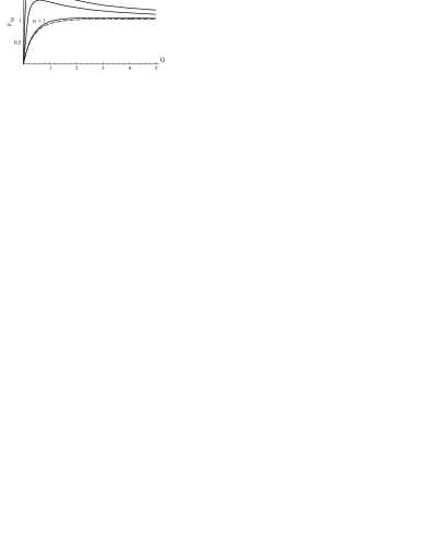
Figure 2: Evolution of the contribution $F_{3d}(Q)$, Eq. (7.28), to the photoconductivity (7.21) with increasing effective microwave power $Q$, Eq. (7.7), for $\alpha=1,\,10,\,30$, and $\beta=0.3$ [Eq. (7.11)]. Dashed curve: the displacement contribution to $F_{3d}(Q)$, given by the first two terms in Eq. (7.27).

The displacement contribution to the function ${\rm F}_{2d}$, shown in Fig. 3(a), is exactly zero, so that ${\rm F}_{2d}$ is entirely due to the contribution of $d_{s}^{(0)}$ and $d_{s}^{(D)}$. At $Q\ll\alpha^{-1}$, ${\rm F}_{2d}$ behaves linearly with $Q$:

$${\rm F}_{2d}\simeq{\alpha Q\over 2}-{2\alpha Q\over 1-\beta^{2}}~{}.$$ (7.31)

The first term in Eq. (7.31) comes from $d_{s}^{(0)}$ and is associated with excitation of the double-frequency harmonics $F_{22}$ and $F_{-2,-2}$ [Eqs. (6.15) and (6.19)]. The second, photovoltaic term, which is due to excitation of $F_{21}$, $F_{01}$, $F_{-2,-1}$, and $F_{0,-1}$, has a larger slope with opposite sign [Eq. (6.22)]. Their behavior at arbitrary $Q$ is illustrated in Fig. 3(b): one can see that each term decreases slowly with increasing $Q$ for $Q\gg\alpha^{-1}$, but they strongly compensate each other, leading to a much faster decay of ${\rm F}_{2d}$.

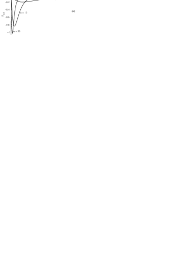
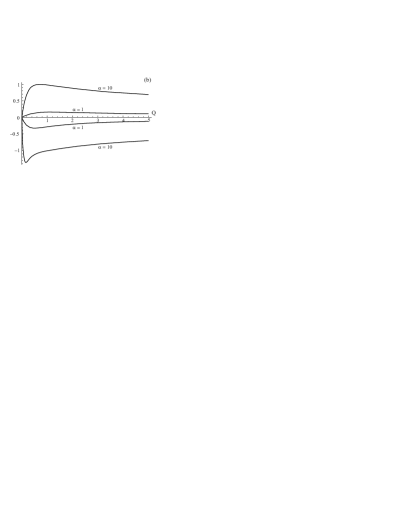
Figure 3: (a) Contribution $F_{2d}(Q)$, Eq. (7.28), to the photoconductivity (7.21) for $\alpha=1,\,10,\,30$, and $\beta=0.3$; (b) “Nonphotovoltaic” (positive) and photovoltaic (negative) contributions to $F_{2d}(Q)$ for $\alpha=1,\,10$.

The function ${\rm F}_{1d}$ is shown in Fig 4(a). It is finite at $Q=0$ and therefore is much larger than both ${\rm F}_{2d}$ and ${\rm F}_{3d}$ at $Q\ll\alpha^{-1}$. The expansion of ${\rm F}_{1d}$ in powers of $Q$ reads:

$${\rm F}_{1d}\simeq 4-9Q-{(\alpha Q)^{2}\over 2}\frac{1+3\beta^{2}}{(1-\beta^{2})^{2}}~{}.$$ (7.32)

The nonzero value of ${\rm F}_{1d}$ at $Q=0$ is due to the saturated inelastic contribution $d_{s}^{(B)}$ [Eq. (6.19)], whereas the linear term comes from both the two-photon correction to the inelastic contribution [Eq. (6.19)] and from the displacement contribution [Eq. (6.20)]. The two contributions related to $d_{s}^{(0)}$ and $d_{s}^{(A)}$ are presented for arbitrary $Q$ in Fig. 4(b). Similarly to ${\rm F}_{3d}$, the photovoltaic term grows quadratically at $Q\ll\alpha^{-1}$. As seen from Fig. 4(b), for $\alpha\gg 1$ it dominates at large $Q$, so that ${\rm F}_{1d}$ changes sign, reaches negative values of order unity, and approaches zero in the limit $Q\to\infty$ from below.

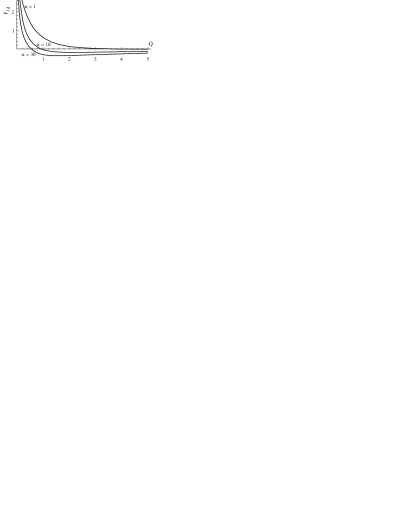
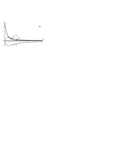
Figure 4: (a) Contribution $F_{1d}(Q)$, Eq. (7.28), to the photoconductivity (7.21) for $\alpha=1,\,10,\,30$, and $\beta=0.3$; (b) Contributions to $F_{1d}(Q)$ [Eq. (7.22)] for $\alpha=1,\,10$: Dashed line: Displacement contribution [third term in Eq. (7.27)]; solid line in the upper half-plane: nonphotovoltaic contribution [second term in Eq. (7.22)]; solid line in the lower half-plane: photovoltaic contribution [third term in Eq. (7.22)].

The functions ${\rm F}_{nh}$ contributing to the Hall part of $\hat{\sigma}_{\rm ph}$ are shown in Fig. 5. All three are related to the photovoltaic mechanism and come from the imaginary part of $g_{1}(x)$ in Eq. (7.26). At $Q\ll\alpha^{-1}$ they grow with increasing microwave power,

$${\rm F}_{1h}\simeq-\frac{2\beta}{1-\beta^{2}}\alpha Q~{},$$ (7.33)

$${\rm F}_{2h}\simeq\frac{2\beta}{(1-\beta^{2})^{2}}(\alpha Q)^{2}~{},$$ (7.34)

$${\rm F}_{3h}\simeq\frac{2\beta}{1-\beta^{2}}\alpha Q~{},$$ (7.35)

and decay to zero in the limit of large $Q$. The maximum values of $|{\rm F}_{nh}|$, which are reached at $Q\sim\alpha^{-1}$, are of order unity (for $\beta\sim 1$), similarly to the behavior of ${\rm F}_{nd}$. It follows that at $Q\sim\alpha^{-1}$ the Hall part $h_{a}$ of the photoresponse becomes as strong as the diagonal part $d_{s}$.

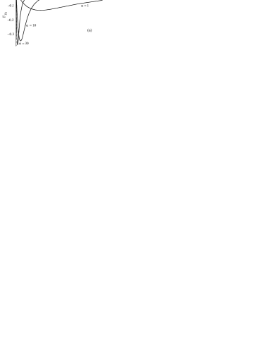
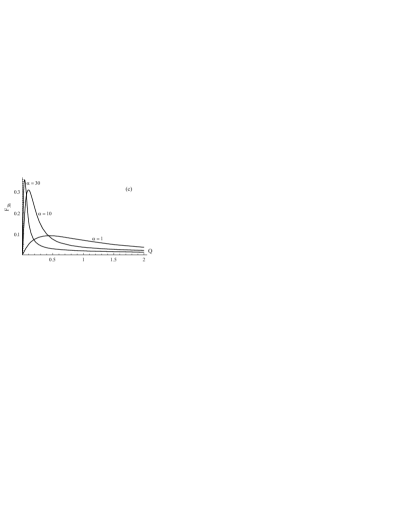
Figure 5: Hall contributions (7.29) to the photoconductivity (7.21) for $\alpha=1,\,10,\,30$, and $\beta=0.3$: (a) $F_{1h}(Q)$; (b) $F_{2h}(Q)$; (c) $F_{3h}(Q)$.

The behavior of $d_{s}$ and $h_{a}$ in the limit of large $Q$ can be found by observing that the main contribution to the integrals (7.23)–(7.26) over $x$ comes then from a close vicinity (of width $Q^{-1/2}$) of points $x=\pi/2$ and $x=3\pi/2$. Around these points the multiphoton processes, which sum up to produce the factors $(1+X_{\omega}^{2})^{-1}$ in Eqs. (7.23)–(7.26), are strongly suppressed. For $Q\gg\alpha^{2}$, the expansion of the factors $\exp(\pm S_{N})$ around unity in Eq. (7.16) yields the asymptotic behavior of the functions ${\rm F}_{nd}$ and ${\rm F}_{nh}$:

$${\rm F}_{1d}\simeq-\frac{7\alpha^{2}}{16Q^{3/2}}~{},$$ (7.36)

$${\rm F}_{3d}\simeq 1+\frac{\alpha^{2}}{8Q^{3/2}}~{},$$ (7.37)

$${\rm F}_{1h}\simeq-\frac{3\beta\alpha}{4Q^{3/2}}~{},$$ (7.38)

$${\rm F}_{3h}\simeq\frac{\beta\alpha}{2Q^{3/2}}~{}.$$ (7.39)

Note that the displacement mechanism gives terms of order $Q^{-3/2}$ in ${\rm F}_{1d}$ and ${\rm F}_{3d}$, which are much smaller than the terms of order $\alpha^{2}Q^{-3/2}$ in Eqs. (7.36) and (7.37) for $\alpha\gg 1$.

In the intermediate interval $\alpha^{-1}\ll Q\ll\alpha^{2}$, where all the functions ${\rm F}_{nd}$ and ${\rm F}_{nh}$, $n=1,2,3$, fall off with increasing $Q$ as a power law, the function $g_{N}(x)$ can be approximated as $g_{N}(x)\simeq{\cal G}_{N}(x)\simeq\Pi_{N}(x)/p(x)$ everywhere except for a vicinity of the singular points $x=\pi/2$ and $x=3\pi/2$. The singular behavior around these points requires special care for the function ${\rm F}_{2d}$, contributions to which coming from $d_{s}^{(0)}$ and $d^{(D)}$ only weakly depend on $Q$ and strongly compensate each other, as illustrated in Fig. 3(b). Consider the part ${\rm F}^{(0)}_{2d}$ related to $d_{s}^{(0)}$:

$${\rm F}^{(0)}_{2d}\simeq{2\over\pi}\int\limits_{0}^{2\pi}\!dx\,\zeta(x)\frac{1-3Q\cos^{2}x}{(1+Q\cos^{2}x)^{3}}~{},$$ (7.40)

where

$$\zeta(x) = \alpha Q\int\limits_{0}^{x}\!dy\frac{\sin y\cos y}{(1+Q\cos^{2}y)^{2}}$$ (7.41)

$$\times \exp\left(-\int\limits_{y}^{x}\!dz\frac{\alpha Q\cos^{2}z}{1+Q\cos^{2}z}\right)~{}.$$

In Eq. (7.40) we neglected the exponentially small (for $Q\gg\alpha^{-1}$) boundary term in the solution (7.15). For $Q\gg\alpha^{-1}$ the main contribution to ${\rm F}^{(0)}_{2d}$ given by Eq. (7.40) comes from the singularities at $x=\pi/2,3\pi/2$. For $Q\ll\alpha^{2}$ one can neglect $Q$ in all the denominators in Eqs. (7.40) and (7.41), after which ${\rm F}^{(0)}_{2d}$ is represented as

$${\rm F}^{(0)}_{2d} \simeq {2\alpha Q\over\pi}\int\limits_{-\infty}^{\infty}\!dx_{1}\int\limits_{-\infty}^{\infty}\!dx_{2}\;x_{1}\,{\rm sgn}(x_{1}-x_{2})$$ (7.42)

$$\times \exp\left(-\alpha Q{|x_{2}^{3}-x_{1}^{3}|\over 3}\right)={4\over\sqrt{3}}~{}.$$

The result does not depend on $Q$, which explains the “plateau” in the behavior of ${\rm F}^{(0)}_{2d}(Q)$ shown in Fig. 3(b). It is important, however, that a similar calculation of the contribution to $F_{2d}$ coming from the photovoltaic term $d_{s}^{(D)}$ exactly cancels the constant term in Eq. (7.42), so that the difference between the two falls off rapidly with increasing $Q$ for $Q\gg\alpha^{-1}$, as observed in Fig. 3(a).

To summarize, in the limit of strongly overlapping Landau levels and low temperatures, $1\ll\alpha\ll\tau_{\rm in}/\tau_{\rm q}$, there appear five regions of $Q$ with essentially different behavior of the photoconductivity as a function of $Q$ and $T$:

• $Q\ll\tau_{\rm q}/\tau_{\rm in}$: the photoresponse is linear in $Q$ and is strongly dependent on $T$;

• $\tau_{\rm q}/\tau_{\rm in}\ll Q\ll 1/\alpha$: the strong feedback effect leads to the saturation of the photoresponse as a function of $Q$. In this interval of $Q$, as well as at higher $Q$, the photoconductivity ceases to depend on $T$;

• $\alpha^{-1}\ll Q\ll 1$: the feedback effects strongly suppress the photoresponse;

• $1\ll Q\ll\alpha^{2}$: the multiphoton effects become important and modify the feedback effects;

• $\alpha^{2}\ll Q$: the photoresponse is dominated by the multiphoton effects, the feedback effects can be treated perturbatively. In the limit $Q\to\infty$ the classical Drude conductivity is restored.

Above, in the bulk of Sec. VII.3, we focused on the case of circular polarization in the limit of high power. Two main differences of linear polarization as compared to circular polarization are as follows. First, the photoresponse becomes anisotropic, i.e., depends on the mutual orientation of ${{\bf E}}_{\omega}$ and ${{\bf E}}_{\rm dc}$. Second, the photoresponse may show much stronger resonant features at $n\omega=2m\omega_{c}$, where $m$ and $n$ are integer numbers. The latter is related to the different structure of perturbation in $(\nu,n)$ space [Eq. (1.1)] induced by the radiation. For the case of passive circular polarization considered above, only the harmonics $F_{2m,2m}$ along the diagonal are excited in the absence of the dc field [they are all contained in the function $g_{0}$ in Eq. (7.8)]. The linear response to the dc field, included in ${\rm St}_{\bot}$, couples these harmonics with their neighbors $F_{2m,2m\pm 1}$. Under the action of ${\rm St}_{j}$ all these harmonics contribute to $F_{\pm 1,0}$ and thus to the dc photoconductivity. In the case of linear polarization, however, all harmonics $F_{2m,n}$, with $m$ and $n$ integer, are excited by radiation, which leads to the “spreading” of the perturbation all over the $(\nu,n)$ plane. The resonances at $n\omega=2m\omega_{c}$ for the case of linear polarization warrant additional study.

VIII Microwave–induced magnetoresistivity oscillations

In Secs. V–VII we have calculated the photoconductivity tensor $\hat{\sigma}_{\rm ph}$ and discussed its evolution with increasing “effective” microwave power $Q$ defined in Eq. (5.17) as

$$Q=P\sin^{2}\frac{\pi\omega}{\omega_{c}}\,\omega^{2}\left[\,{s_{+}^{2}\over(\omega_{c}+\omega)^{2}}+{s_{-}^{2}\over(\omega_{c}-\omega)^{2}}\,\right]~{},$$ (8.1)

where

$$P=\frac{2\tau_{\rm q}}{\tau_{\rm tr}}\left(\frac{eE_{\omega}v_{F}}{\omega^{2}}\right)^{2}~{}.$$ (8.2)

However, what is usually measured in the experiment is the photoresistivity $\hat{\rho}_{\rm ph}$ as a function of $\omega_{c}$ at fixed $\omega$ and $P$. The dependence of $\hat{\rho}_{\rm ph}$ on $\omega_{c}/\omega$ for a given $P$ is discussed below, assuming, as in Secs. VII.2 and VII.3, passive circular polarization of the microwave field.

For circular polarization, the photoresistivity tensor is easily obtained in the limit of classically strong magnetic field, $\omega_{c}\tau_{\rm tr}\gg 1$, by inverting Eq. (7.21):

$$\hat{\rho}_{\rm ph} \simeq {1\over 2\sigma^{\rm D}_{xx}(\omega_{c}\tau_{\rm tr})^{2}}$$ (8.5)

$$\times \left(\!\begin{array}[]{cc}1+2\delta^{2}(1-d_{s})&\omega_{c}\tau_{\rm tr}-2\delta^{2}h_{a}\\ -\omega_{c}\tau_{\rm tr}+2\delta^{2}h_{a}&1+2\delta^{2}(1-d_{s})\end{array}\!\right)~{}.$$

Here we neglect a small admixture of $-4\delta^{2}h_{a}/\omega_{c}\tau_{\rm tr}$ in the diagonal part of $\hat{\rho}_{\rm ph}$, as well as a similar admixture of $\pm 4\delta^{2}d_{s}/\omega_{c}\tau_{\rm tr}$ in the Hall part.

It was shown in Sec. VII that, while in the linear regime with respect to the microwave power the inelastic contribution to the photoresponse dominates, already at $Q\sim\alpha^{-1}\sim 1$ the inelastic and photovoltaic contributions become comparable in magnitude. The displacement contribution becomes also relevant at this power if $\alpha\sim 1$. The interplay of the three contributions in the traces of $d_{s}$ and $h_{a}$ as a function of the ratio $\omega_{c}/\omega$ is illustrated in Figs. 6–9 for the case of passive circular polarization. The dependence of $d_{s}$ and $h_{a}$ on $\omega_{c}$ is shown over a single period of oscillations around the second harmonic of the cyclotron resonance for $2/5<\omega_{c}/\omega<2/3$. Each of Figs. 6–9 corresponds to one of four values of the microwave power $P=0.01,\,0.1,\,1$, and 10.

Within each of Figs. 6–9 two cases are illustrated, corresponding to two different values of the parameter $\alpha$ [Eq. (7.11)] taken at $\omega_{c}/\omega=1/2$. In every figure, (a) and (b) correspond to $\alpha_{1/2}=(3\omega_{c}\tau_{\rm q})^{-1}=1$, while (c) and (d) to $\alpha_{1/2}=10$. In all the figures we take the same ratio $\tau_{\rm in}/\tau_{\rm q}=50$, thus neglecting the heating effect, discussed separately in Sec. IX.2.

Figure 6: Diagonal, $d_{s}$, and Hall, $h_{a}$, parts of the magnetoresistivity tensor (LABEL:rhoph) at moderate microwave power $P=0.01$ [Eq. (8.2)] vs $\omega_{c}/\omega$. Solid lines: the functions $-d_{s}$ [panels (a) and (c)] and $h_{a}$ [panels (b) and (d)]; (a) and (b) correspond to $\alpha_{1/2}=1$, while (c) and (d) to $\alpha_{1/2}=10$. Dashed lines: the linear–in–$P$ asymptotes $d_{s}^{(B)}+d_{s}^{(D)}$ and $h_{a}^{(D)}$ [Eqs. (5.23), (5.24), and (5.29)].

Figure 7: Solid lines: same as in Fig. 6 for $P=0.1$. Dashed lines: the asymptote for $h_{a}$ in the SIC regime [Eq. (LABEL:haha)]. Dotted lines: the saturated inelastic contribution [Eq. (6.6)].

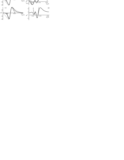
Figure 8: Solid lines: same as in Fig. 7 for $P=1$. Dashed lines: the asymptotes for $d_{s}$ and $h_{a}$ in the SIC regime [Eqs. (8.8) and (LABEL:haha)]. Dotted lines: the saturated inelastic contribution [Eq. (6.6)].

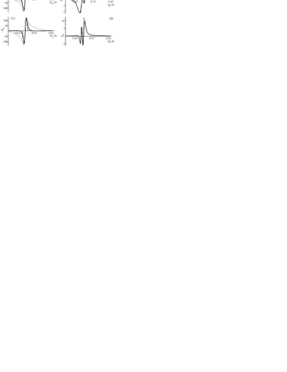
Figure 9: Same as in Fig. 8 for $P=10$.

At $P=0.01$ (Fig. 6), not only $Q$ but also $Q_{\rm in}=\tau_{\rm in}Q/2\tau_{\rm q}$ is small compared to unity in the whole interval $2/5<\omega_{c}/\omega<2/3$. Therefore, the photoresponse is well described by the linear-in-$P$ asymptotes (5.21)–(5.29). More specifically, the diagonal part at $\alpha\sim 1$ is dominated by the inelastic contribution $d_{s}^{(B)}$ [Eq. (5.23)], while at $\alpha\gg 1$ the photovoltaic contribution $d_{s}^{(D)}$ [Eq. (5.24)] becomes pronounced near the ends of the interval (where inelastic contribution vanishes, $\cot w=0$). The Hall response is governed by the photovoltaic contribution $h_{a}^{(D)}$ [Eq. (5.29)]. The displacement part $d_{s}^{(A)}$ is small due to the large ratio $\tau_{\rm in}/\tau_{\rm q}=50$, while the quadrupole contribution to the Hall part, $h_{s}^{(C)}$ [Eq. (5.28)], as well as the anisotropic diagonal part (5.25) are absent for circular polarization. In the case of linear polarization, $h_{s}^{(C)}$ would provide a Hall contribution of the same order of magnitude as $h_{a}^{(D)}$. For comparison, the linear asymptotes $d_{s}^{(B)}+d_{s}^{(D)}$ and $h_{a}^{(D)}$ are shown in Fig. 6 by the dashed lines. The mismatch between the solid and dashed lines is negligible for small detuning from the resonance,

$$\Delta\equiv|\omega/\omega_{c}-2|\ll 1~{},$$ (8.7)

owing to the $\sin^{2}\pi\Delta$ term in Eq. (8.1). Away from the resonance, at $\Delta\sim 1/2$, the parameter $Q_{\rm in}\simeq 0.1$ and the feedback effects (Sec. VI) lead to a noticeable correction to the linear behavior.

The evolution of $d_{s}$ and $h_{a}$ with increasing $P$ reveals the nonlinear effects studied in Secs. VI and VII. First of all, note that the part of $\hat{\sigma}_{\rm ph}$ associated with ${\rm F}_{1d}$ and ${\rm F}_{1h}$ [Eqs. (7.28) and (7.29)] vanishes both at $\Delta=0$ and at $\omega_{c}/\omega=2/5$ and $2/3$, where $\Delta=1/2$. The photoresponse at both ends of the interval is, therefore, fully governed by the contributions to $\hat{\sigma}_{\rm ph}$ coming from ${\rm F}_{2d}$, ${\rm F}_{3d}$, ${\rm F}_{2h}$ and ${\rm F}_{3h}$, which represent subleading terms for small $P$. In accord with the results of Sec. VII, Figs. 7(a) and (c) show that the photoresponse at $\Delta=1/2$ in $d_{s}$ is indeed discernible only at $P\gtrsim\alpha^{-1}$; otherwise, it is masked by the much stronger inelastic contribution that develops at $\Delta<1/2$.

In the vicinity of the resonance, the diagonal photoresistivity is dominated by the $F_{1d}$ term in Eq. (7.28), which at $\Delta^{2}\ll(P\alpha)^{-1}$ can be represented as

$$d_{s}\simeq w\cot w\,{\rm F}_{1d} \simeq {2\pi\omega\over\omega_{c}}\frac{P^{*}_{\rm in}\sin(2\pi\omega/\omega_{c})}{1+P^{*}_{\rm in}\sin^{2}(\pi\omega/\omega_{c})}$$ (8.8)

$$- {9\pi\omega\over 2\omega_{c}}\,P^{*}\sin{2\pi\omega\over\omega_{c}}$$

$$- {\pi\omega\over 4\omega_{c}}\sin{2\pi\omega\over\omega_{c}}\left(\frac{P^{*}}{\omega\tau_{\rm q}}\sin{\pi\omega\over\omega_{c}}\right)^{2}$$

$$\times \frac{(\omega+\omega_{c})^{2}+3\omega_{c}^{2}}{(\omega+2\omega_{c})^{2}}~{},$$

where

$$P^{*}=P\frac{\omega^{2}}{(\omega+\omega_{c})^{2}}~{},\qquad P^{*}_{\rm in}=\frac{\tau_{\rm in}}{2\tau_{\rm q}}P^{*}~{},$$ (8.9)

see Eqs. (6.18), (6.20), and (7.32). The asymptote (8.8) is shown in panels (a) and (c) of Figs. 8 and 9 by the dashed line, while the dotted line describes the behavior of the first term of Eq. (8.8), which represents the saturated inelastic contribution [Eq. (6.6), see also Eq. (15) of Ref. long, ]. For $P\gg\alpha^{-1}$ the photoresponse tends to concentrate at $\Delta\ll 1$, which can be seen from its evolution with increasing $P$ in Figs. 6–9.

Similarly, the Hall part at $\Delta^{2}\ll(\alpha P)^{-1}$ can be approximated by

$$h_{a} \simeq \frac{2\omega_{c}P^{*}\sin^{2}(\pi\omega/\omega_{c})}{\omega\tau_{\rm q}(\omega+2\omega_{c})}$$

$$+ 2\pi\left(1+{\omega_{c}\over\omega}\right)\left(\frac{P^{*}\sin^{2}(\pi\omega/\omega_{c})}{(\omega+2\omega_{c})\tau_{\rm q}}\right)^{2}$$

$$- \frac{\pi P^{*}\sin(2\pi\omega/\omega_{c})}{(\omega+2\omega_{c})\tau_{\rm q}}\;\frac{1-P^{*}_{\rm in}\sin^{2}(\pi\omega/\omega_{c})}{1+P^{*}_{\rm in}\sin^{2}(\pi\omega/\omega_{c})}~{},$$

see Eqs. (6.10), (7.34), and (5.18). The asymptote (LABEL:haha) is shown in panels (b) and (d) of Figs. 7–9 by the dashed line.

Let us now briefly recall the physics behind the calculated dependencies by the example of Fig. 9, where the microwave power $P=10$ is large and the effective power $Q$ [Eq. (8.1)] changes from $Q=0$ at $\omega_{c}/\omega=1/2$ to $Q\sim 10$ at $\omega_{c}/\omega=2/5$ and $2/3$. As a result, in Fig. 9, the system passes with increasing $\Delta$ through all regimes discussed in Secs. V–VII.

• $\Delta=0$: exactly on resonance, the photoresponse is zero.

• $\Delta\ll\Delta_{\rm max}\ll 1$: the linear photoresponse, $d_{s},\,h_{a}\propto P\Delta$ (Sec. V). The inelastic contribution dominates the photoresponse in the diagonal part,

  $$d_{s}=-{8\over 9}\,(2\pi)^{2}\,{\tau_{\rm in}\over\tau_{\rm q}}\,P\Delta$$ (8.11)

  [linear–in–$P$ part of the first term in Eq. (8.8)], while in the Hall part the photovoltaic mechanism produces

  $$h_{a}=-{1\over 3}(2\pi)^{2}\,\alpha_{1/2}\,P\Delta~{},$$ (8.12)

  [linear–in–$P$ part of the last term in Eq. (LABEL:haha)]. The maximum value of the inelastic term in $d_{s}$ as a function of $\Delta$ is reached at

  $$\Delta_{\rm max}\equiv\sqrt{9\tau_{\rm q}/2\pi^{2}\tau_{\rm in}P}~{}.$$ (8.13)

• $\Delta\sim\Delta_{\rm max}$: the crossover to the SIC regime (Sec. VI). As detuning from the resonance $\Delta$ approaches $\Delta_{\rm max}$, the nonlinear corrections in the first term of Eq. (8.8) and in the last term of Eq. (LABEL:haha), driven by the feedback effects related to the strong oscillatory pattern in the isotropic part $F_{00}(\varepsilon)$ of the distribution function, become important. At $\Delta=\Delta_{\rm max}$, the inelastic contribution to $d_{s}$ reaches maximum, $d_{s}=\pm 4\Delta_{\rm max}^{-1}\propto\sqrt{P}$, and crosses over into the $\Delta^{-1}$ decay at $\Delta>\Delta_{\rm max}$ (illustrated by the dotted lines). In the Hall term $h_{a}$, the strong oscillations of $F_{00}$ change sign of the photovoltaic contribution at $\Delta=\Delta_{\rm max}$.

• $\Delta_{\rm max}\ll\Delta\ll(P\alpha)^{-1/2}:$ the SIC regime, in which the photoresponse becomes independent of $\tau_{\rm in}$ and, hence, on temperature. This property of the high–power photoresponse can be easily verified experimentally.

  At $\Delta\gg\Delta_{\rm max}$, the two last terms in Eq. (8.8) become relevant, leading to a decrease of the diagonal photoresponse. The last term is actually irrelevant in Fig. 9(a) (which corresponds to $\alpha_{1/2}=1$), so that [Eq. (7.32)]:

  $$d_{s}\simeq\frac{\pi\omega}{\omega_{c}}\cot\frac{\pi\omega}{\omega_{c}}(4-9Q)\simeq{8\over\Delta}-8\pi^{2}P\Delta~{}.$$ (8.14)

  The second term in Eq. (8.14) consists of the displacement contribution modified by the strong oscillations in $F_{00}$ [in the SIC regime, its sign is inverted compared to the linear case, Eq. (6.12)] and the two–photon correction to $F_{00}$ itself [Eq. (5.3)]. This term is responsible for the strong narrowing of the oscillation in $d_{s}$ as a function of $\Delta$ and also for the nonmonotonic dependence on power at fixed $\Delta$. At $\alpha\gg 1$, the last, photovoltaic term in Eq. (8.8) becomes important, leading to additional narrowing of the peak in Fig. 9(c) and Fig. 8(c) compared to Fig. 9(a) and Fig. 8(a).

  The Hall part $h_{s}$ exhibits an additional oscillation at $\Delta\sim(P\alpha)^{-1/2}$ and decays for larger $\Delta$ due to the feedback and multiphoton effects. At $\Delta\gg\Delta_{\rm max}$, the first two terms in Eq. (LABEL:haha) (which, in contrast to the last term, are even in detuning $\omega-2\omega_{c}$ from the resonance) become pronounced, as can be seen, for example, from the difference in amplitude of the second peak and the second dip in Fig. 9(d).

• $\Delta\gg(P\alpha)^{-1/2}$: the ultrahigh power regime, in which all effects related to the Landau quantization decay to zero due to the feedback and multiphoton effects.

Figures 6–9 demonstrate that, for large $P$ and/or large $\alpha$, the strongly nonlinear effects studied in Sec. VII essentially modify the behavior characteristic of the SIC regimelong (dotted lines in Fig. 7–9). In particular, high–power measurements should reveal the significant narrowing of the oscillation in $\rho_{xx}$ with increasing $P$, manifest in Figs. 8 and 9. It should be noted that, in addition to the magnetoresistivity traces dominated by the strong feature in the vicinity of $\Delta=0$, it is worth studying the $Q$ and $T$–dependences of the photoresponse at several fixed ratios $\omega/\omega_{c}$; in particular, the contributions ${\rm F}_{2d}$ and ${\rm F}_{3d}$ which manifest themselves at $\Delta\sim 1/2$.

At $P\sim\alpha^{-1}$ the magnitude of the photoresponse in $\rho_{xy}$, Fig. 7(d), becomes comparable to the effect in $\rho_{xx}$, Fig. 7(c), which seems to be in accord with the experiment.maniHall However, the experiments that revealed the Hall oscillations with $h_{a}\simeq-d_{s}$ were performed at $\omega\tau_{\rm q}\sim 1$, i.e., at $\alpha\sim 1$, where for the level of power used in the experiment the predicted oscillations in $h_{a}$ should be more than an order of magnitude smaller than those in $d_{s}$. Our theory is not capable of explaining the observed effect in $\rho_{xy}$ (probably related to microwave–induced $\omega/\omega_{c}$–dependent changes in the electron concentration, see discussion in Sec. VIII of Ref. long, ).

IX Range of applicability of the theory

The above calculation the OPC is based on the assumptions that (i) disorder is smooth, Eq. (2.2); (ii) temperature is high, Eq. (3.3); (iii) Landau levels strongly overlap with each other, Eq. (4.1). Altogether, these conditions made the analytical treatment of the problem possible to all orders in the microwave power. Now let us briefly discuss the range of applicability of the above approximations, especially in the limit of strongly nonlinear photoresponse. In particular, it is important to discuss the role of heating.

IX.1 Heating effects

The high–$T$ approximation led us to Eq. (3.3) for the oscillatory distribution function (see Appendix A). The Fermi–Dirac part of the distribution is characterized by the effective temperature $T_{e}\gg\omega_{c}$. The oscillatory part appears due to the Landau quantization, which, in the limit of strongly overlapping Landau levels, is weak: the amplitude of the oscillations of the DOS is proportional to the small parameter $\delta$ [Eq. (4.1)]. The heating of electrons, which leads to a growth of $T_{e}$ with increasing microwave power, can therefore be treated separately within the framework of the classical Boltzmann equation with a constant DOS. Such a calculation leads to the following equation for $T_{e}$:classical

$$(T_{e}/T_{0})^{4}\,(T_{e}/T_{0}-1)=\eta~{},$$ (9.1)

$$\eta={\tau_{\rm e-ph}(T_{0})\over\tau_{\rm tr}}\,\left(\frac{ev_{F}E_{\omega}}{2T_{0}}\right)^{2}\,\sum\limits_{\pm}\left(\frac{s_{\pm}}{\omega\pm\omega_{c}}\right)^{2}~{}.$$

(9.2)

Here $\tau_{\rm e-ph}^{-1}(T_{0})\propto T_{0}^{3}$ is the inelastic relaxation rate due to scattering on acoustic phonons (the latter represent a thermal bath at temperature $T_{0}$) and $s_{\pm}$ describes polarization of microwaves [Eq. (2.20)]. At a typical value of $T_{0}\sim 1$ K, the electron–phonon scattering rate exceeds $\tau_{\rm tr}^{-1}$ by more than an order of magnitude, so that the parameter $\eta$ in Eq. (9.2) can vary between 1 and 1000 under realistic experimental conditions. At first glance, the large values of $\eta$ imply a strong heating, $T_{e}\gg T_{0}$. However, this is not actually the case in view of the strong temperature dependence of $\tau_{\rm e-ph}(T)$. While at $\eta\lesssim 1$ the temperature grows linearly with $\eta$ (specifically, $T_{e}-T_{0}\simeq\eta$), in the limit of strong heating the growth is much weaker, $T_{e}/T_{0}\simeq\eta^{1/5}\gg 1$. The weak dependence on the microwave power at large $\eta$ means that, in practice, the heating can be substantial but never strong, i.e., $T_{e}/T_{0}\sim 2\div 3$. At the same time, with lowering bath temperature well below $1\,$K, while keeping the microwave power constant, the heating effect may become significantly more pronounced (since $\eta$ grows with lowering temperature as $T_{0}^{-5}$), in effect restoring the high–$T$ limit we deal with in the paper.

In the dc response, the strongest manifestation of the heating effect is the exponential suppression of the Shubnikov-de Haas oscillations (provided the latter are visible in the absence of microwaves at $T_{e}=T_{0}$). The OPC is influenced much more weakly, since $T_{e}$ enters the photoconductivity only indirectly, through the $T$–dependence of the electron-electron inelastic scattering rate, $\tau_{\rm in}^{-1}\propto T_{e}^{2}$. In particular, in the linear regime, $P\ll\tau_{\rm q}/\tau_{\rm in}$, taking the heating effects into account leads to a sublinear dependence of the diagonal photoresponse on the microwave power, namely $d_{s}\propto PT_{e}^{-2}(P)$, while at high power, $P\gg\tau_{\rm q}/\tau_{\rm in}$, the maxima and minima of $d_{s}$ scale as $\sqrt{P}/T_{e}(P)$.

IX.2 Stratification of the distribution function

Apart from the condition on the temperature $T_{e}\gg 1/t_{B}$, the approximation (3.3) is valid only if the oscillatory correction to the distribution function remains much smaller than unity, so that the general requirement $0<f(\varepsilon)<1$ is met. Despite the DOS being only weakly modulated ($\delta\ll 1$), the above condition is violated at sufficiently high power for the values of the ratio $\omega/\omega_{c}$ corresponding to the minima and maxima of $d_{s}$ [see Figs. 9(a) and (c)]. Near these points, the effect is governed by the inelastic mechanism, Eq. (8.14), and the oscillatory part of Eq. (3.3) can be estimated as

$${\cal F}(\varepsilon)\,\partial_{\varepsilon}f_{T}\sim\frac{\delta\,d_{s}}{t_{B}\,T_{e}}\sin(\varepsilon t_{B})\lesssim\frac{\delta}{t_{B}\,T_{e}\,\Delta_{\rm max}}~{},$$ (9.3)

where we used Eqs. (4.3), (4.7), (6.4), (6.6), and (8.14).

At large power, the maximum value of $d_{s}$ grows as $\sqrt{P}/T_{e}(P)$ [see Eq. (8.11) at $\Delta=\Delta_{\rm max}$]. It follows that at $P\sim P_{\star}=(\omega_{c}\delta/T_{e})^{2}\tau_{\rm in}/\tau_{\rm q}$ the oscillations of the isotropic part of the distribution near the maxima and minima of $d_{s}$ become of order unity. At small detuning from the cyclotron resonance harmonics, $\Delta\sim\Delta_{\rm max}$, and at $P>P_{\star}$, the splitting of $f(\varepsilon)$ into the smooth and oscillatory parts (3.3) is no longer possible. The distribution function in this regime can be calculated numerically according to Eq. (11) of Ref. long, (for details of the numerical procedure, see Ref. crossover, ). An illustrative example of the stratification of the distribution function at $P\sim P_{\star}$ is shown in Fig. 10. Both the heating and the stratification of the distribution function suppress the growth and the narrowing of the peak in $d_{s}$ at very high power. Beyond the close vicinity of maxima and minima, at $|\Delta|=|\omega/\omega_{c}-N|\gg\delta/t_{B}\,T_{e}$ (where $N$ is integer), the oscillatory correction to the distribution function remains small at any power level and the high–$T$ approximation works well, so that our results remain intact whatever the microwave power.

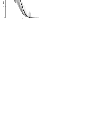
Figure 10: Isotropic part of the distribution function at three levels of the microwave power: $P=0$, $P\ll P_{\star}$, and $P\sim P_{\star}$.

IX.3 Smooth vs short–range disorder

In this paper we assumed that the disorder potential is created solely by charged impurities separated from the plane of the 2DEG by a spacer of width $\xi/2\gg k_{F}^{-1}$ [Eq. (2.2)]. Such a minimal model of disorder allowed us to account for the experimentally relevant small–angle scattering condition $\tau_{\rm q}\gg\tau_{\rm tr}$ and to consider in an unambiguous way the region of magnetic fields $\tau_{\rm tr}^{-1}\ll\omega_{c}\ll\tau_{\rm q}^{-1}$. On the other hand, a “two–component model” of disorder,twocomponent including strong scatterers on the background of the smooth potential (2.2), is known to provide a better description of real ultrahigh–mobility structures.

To our current understanding, the inclusion of the strong scatterers into the theory should not lead to any qualitative change of the results presented here [provided the conditions (2.1) remain satisfied]. In particular, the derivation of the linear-order inelastic contribution (5.23) in Ref. dmitriev03, does not require any assumptions as to the type of disorder.

By contrast, the strong scatterers were shownyang02 ; 2componentDC to play a crucial role in the nonlinear dc response (in the absence of microwaves), where strong oscillations of the magnetoresistivity (“HIRO”) were observed,yang02 ; bykov1 ; bykov2 ; inelasticDC ; strongDC governed by the ratio of the Hall electric field to the magnetic field. Remarkably, a strong interplay between two types of oscillations in the 2DEG driven by both microwave and strong dc fields was recently observed experimentally.ACDC Theoretical description of this experimental situation necessitates the inclusion of the backscattering off strong impurities, which we relegate to future work. It was argued in Ref. Volkov, that, in the regime of strong dc field and in the presence of short range disorder, effects of the microwave field on screening of impurities should also be taken into account.

IX.4 Stronger magnetic fields, $\omega_{c}\tau_{\rm q}\gtrsim 1$

The calculations in Secs. V-VII were performed for the case of strongly overlapping Landau levels, $\omega_{c}\tau_{\rm q}\ll 1$. In this limit, (i) microwave-induced corrections to the DOS can be neglected; (ii) there are substantial effects related to excitation of higher angular and temporal harmonics of the distribution function; in particular, the photovoltaic and quadrupole contributions to the OPC. At stronger magnetic fields, the modulation of the DOS due to the Landau quantization becomes more pronounced: in the SCBA approximation, at $\omega_{c}\tau_{\rm q}\simeq 1.8$ the Landau levels get separated from each other.crossover For the case of separated Landau levels, the effect on higher harmonics of the distribution function becomes strongly suppressed and the diagonal part of the photoresponse is determined by the interplay of the inelastic and displacement mechanisms.

In addition to the nonlinear effects considered in this paper, at $\omega_{c}\tau_{\rm q}\gtrsim 1$ the DOS itself is modified by microwave radiation. In particular, microwave–induced sidebands appear on both sides of the Landau levels, leading to the appearance of an additional structure in the OPC pattern near the fractional harmonics of the cyclotron resonance, $n\omega=m\omega_{c}$.separated A similar structure in photoresponse also arises as a multiphoton correction to the inelastic contribution to the OPC. Both structures have precisely the same shape (as a function of $\omega$); however, the multiphoton mechanism dominates in the case of strongly separated Landau levels.separated Such a “fractional oscillatory pattern” (FOP) in the nonlinear photoresponse was observed in recent experimentszudov04 ; multi ; dorozhkin06 and explained in terms of either of multiphoton corrections to the displacement contributionzudov04 ; multi ; leiliumulti or, alternatively, in terms of single–photon resonant corrections to the inelastic contribution which are specific to the crossover region $\omega_{c}\tau_{\rm q}\sim 1$.dorozhkin06 ; crossover All four contributions to the FOP will be compared and analyzed elsewhere.separated

X Conclusions

Summarizing, we have developed the systematic approach to the microwave–induced oscillations in the magnetoresistivity of a 2DEG. This approach has enabled us to classify contributions to the photoresistivity according to the combined action of the microwave and dc fields on the temporal and angular harmonics of the distribution function (Sec. III). We have studied the interplay of the resulting mechanisms of photoresponse at high microwave power. In the limit of strongly overlapping Landau levels (Sec. IV), the dc photoconductivity has been calculated to all orders in the microwave power (Sec. V–VII).

To linear order in the power, two novel mechanisms of the oscillations (quadrupole and photovoltaic) have been identified, in addition to the known ones (displacementryzhii and inelasticdmitriev03 ). The quadrupole and photovoltaic mechanisms have been shown to be the only ones leading to oscillations in the Hall part of the photoconductivity tensor. Of particular interest is the result that the quadrupole contribution violates Onsager symmetry. In the diagonal part, the inelastic contribution dominates at moderate microwave power, while at elevated power the contributions of other mechanisms become important.

In Secs.VI and VII we have considered the strongly nonlinear photoresponse at high microwave power. We have shown that a competition between various nonlinear effects (the feedback effects, the excitation of high angular and temporal harmonics of the distribution function, and the multiphoton effects) drives the system through four different nonlinear regimes with increasing microwave power.

Most dramatic changes in the photoresponse are due to the feedback effects. In the SIC regime, Sec.VI, the feedback from the microwave–induced oscillations of the isotropic part of the distribution, $F_{00}$, leads to the saturation of the inelastic contribution,short ; long and to the strong interplay of the inelastic effect and all other contributions to the OPC. In particular, the strong oscillations of $F_{00}$ change sign of the most relevant parts of the displacement and photovoltaic contributions. Remarkably, in the SIC regime the photoresponse becomes independent of the inelastic scattering rate and, therefore, of temperature.

At higher power, Sec. VII, the feedback suppresses the effects on higher temporal and angular harmonics of the distribution function. At still higher power, the multiphoton excitation becomes pronounced and starts to compete with the feedback effects. At ultrahigh power, the feedback and multiphoton effects destroy all quantum contributions, restoring the classical Drude conductivity.

Our theory predicts nonmonotonic behavior of the diagonal photoresponse as a function of the microwave power at a fixed ratio $\omega/\omega_{c}$. As illustrated in Sec. VIII, in magnetoresistivity measurements such a nonmonotonic dependence should result in a significant narrowing of the oscillatory structure around the integer values of $\omega/\omega_{c}$ at sufficiently large power, see Eq. (8.14). To a large extent, the narrowing is due to the displacement contribution. At the same time, the amplitude of the oscillations is controlled by the inelastic mechanism at any power level. We suggest to experimentally measure the power and temperature dependences of the photoresponse at fixed $\omega/\omega_{c}$ not too close to the cyclotron resonance harmonics. Such experiments will make it possible to observe the rich behavior of the photovoltaic contributions. Also, our theory predicts oscillations in $\rho_{xy}$, which, in the limit of strongly overlapping Landau levels, can be comparable in amplitude with those in $\rho_{xx}$.

We thank S.I.Dorozhkin, R.R. Du, K. von Klitzing, J.H. Smet, and especially M.A. Zudov for information about the experiments, D.N. Aristov, A.P. Dmitriev, and I.V. Gornyi for stimulating discussions, and E.E. Takhtamirov and V.A. Volkov for sending us the paper Ref. Volkov, prior to publication. This work was supported by the SPP “Quanten-Hall-Systeme” and Center for Functional Nanostructures of the DFG, by INTAS Grant No. 05-1000008-8044, and by the RFBR.

Appendix A Quantum Boltzmann equation in the high-temperature limit

In this Appendix we derive the high–$T$ version of the quantum Boltzmann equation starting from its general form, Eqs. (2.11), (2.13). We show that the solution of the QBE in the limit $T\gg\omega_{c}$ has the form

$$f_{21}\equiv f(t_{-},\,t)={\cal G}(t_{-})+\sum\limits_{n=-\infty}^{\infty}\Phi_{n}(\varphi,t)\,it_{-}^{(n)}{\cal G}(t_{-}^{(n)})$$ (A.1)

and obtain the equations for the amplitudes $\Phi_{n}(\varphi,t)$. Here $t_{-}=t_{2}-t_{1}$, $t=(t_{2}+t_{1})/2$, and ${\cal G}(t_{-})=(2\pi)^{-1}\int\!d\varepsilon\,f_{T}(\varepsilon)\exp(-i\varepsilon t_{-})$ is the Fermi distribution function in the time representation,

$${\cal G}(t_{-})=\frac{i\,T\exp(-i\varepsilon_{F}t_{-})}{2\sinh\pi T(t_{-}+i0)}\,,\qquad t_{-}^{(n)}=t_{-}-nt_{B}~{}.$$

In the energy representation, the solution (A.1) acquires the form (3.3),

$$f(\varepsilon,\varphi,t) = \int\!dt_{-}\,e^{i\varepsilon t_{-}}f_{21}$$ (A.2)

$$= f_{T}(\varepsilon)+{\cal F}(\varepsilon,t,\varphi)\,\partial_{\varepsilon}f_{T}(\varepsilon)~{},$$

$${\cal F}(\varepsilon,\varphi,t) = \sum\limits_{n=-\infty}^{\infty}\Phi_{n}(\varphi,t)\,\exp(in\varepsilon t_{B})~{}.$$ (A.3)

In the high–$T$ limit, the function $f(\varepsilon)$ shows fast oscillations on top of the smooth thermal distribution $f_{T}(\varepsilon)$. The function $f_{21}$, Eq. (A.1), is composed of equidistant sharp peaks of width $1/T$, with the distance between them being equal to $t_{B}$.

The DOS (3.1) for high Landau levels is a periodic function of energy and the functions $g^{R}=-\left(g^{A}\right)^{\dagger}$, entering Eq. (2.13), obey

$$g^{R}_{21}=\sum\limits_{m=0}^{\infty}\,g_{m}(t)\,\delta(t_{-}^{(n)})~{}.$$ (A.4)

In terms of the coefficients $g_{m}$, the QBE is rewritten as

$$(\partial_{t}+\omega_{c}\partial_{\varphi})f_{31}-{\rm St}_{\rm in}\{f\}_{31}={\rm St}_{\rm im}\{f\}_{31}$$ (A.5)

with

$${\rm St}_{\rm im}\{f\}_{31} = \sum\limits_{m\geq 0}\left[\,\hat{\cal K}_{31}g_{m}\left(\!\frac{t_{2}+t_{3}}{2}\!\right)f_{21}-f_{21}\hat{\cal K}_{32}g_{m}\left(\!\frac{t_{2}+t_{3}}{2}\!\right)\,\right]_{t_{2}=t_{3}-mt_{B}}$$ (A.6)

$$+ \sum\limits_{m\geq 0}\left[\,\hat{\cal K}_{31}f_{32}g_{m}^{*}\left(\!\frac{t_{2}+t_{1}}{2}\!\right)-f_{32}\hat{\cal K}_{21}g_{m}^{*}\left(\!\frac{t_{2}+t_{1}}{2}\!\right)\,\right]_{t_{2}=t_{1}-mt_{B}}~{}.$$

Now we substitute the solution in the form (A.1) into the kinetic equation. The unperturbed part ${\cal G}(t_{-})$ gives zero on the l.h.s. of Eq. (A.5). The impurity collision integral acting on ${\cal G}(t_{-})$, produces

$${\rm St}_{\rm im}\{{\cal G}\}_{31} = \sum\limits_{m\geq 0}\left.{\cal G}(t_{2}-t_{1})[\hat{\cal K}_{31}-\hat{\cal K}_{32}]g_{m}(t_{3}-mt_{B}/2)\right|_{t_{3}-t_{2}=mt_{B}}$$ (A.7)

$$+ \sum\limits_{m\geq 0}\left.{\cal G}(t_{3}-t_{2})[\hat{\cal K}_{31}-\hat{\cal K}_{21}]g_{m}^{*}(t_{1}-mt_{B}/2)\right|_{t_{1}-t_{2}=mt_{B}}~{},$$

where we took into account the fact that the operator $\hat{\cal K}$, in the time representation, commutes with an arbitrary function independent of $\varphi$, see Eq. (2.25). Let us consider the first sum in the above expression. At $Tt_{B}\gg 1$, the $\delta$-function-like ${\cal G}(t_{2}-t_{1})$ puts $t_{2}$ within the interval $|t_{2}-t_{1}|\lesssim 1/T$. Strictly at the point $t_{2}-t_{1}=0$, the function ${\cal G}(t_{2}-t_{1})$ is infinite, while the expression in the square brackets is zero. Recalling that the kernel changes smoothly on the scale of $|t_{2}-t_{1}|\sim 1/T\ll t_{B}$, one can replace the difference in the brackets by the derivative $\partial_{1}\hat{\cal K}_{31}$. The result is a series of peaks of identical shape,

$${\rm St}_{\rm im}\{{\cal G}\}_{21}=\sum\limits_{-\infty}^{\infty}{\cal A}_{N}(t)\,it_{-}^{(n)}{\cal G}(t_{-}^{(n)})~{},$$

$${\cal A}_{N>0}=-i\left[\,(\partial_{t_{-}}-\partial_{t}/2)\hat{\cal K}_{21}\,\right]_{t_{-}=Nt_{B}}\,g_{N}(t)~{},$$

$${\cal A}_{N<0}=-i\left[\,(\partial_{t_{-}}+\partial_{t}/2)\hat{\cal K}_{21}\,\right]_{t_{-}=Nt_{B}}\,g^{*}_{-N}(t)~{},$$

$${\cal A}_{N=0}=-2i\left[\,\partial_{t_{-}}\hat{\cal K}_{21}\,\right]_{t_{-}=0}g_{0}=-i\left.\partial_{t_{-}}\hat{\cal K}\right|_{t_{-}=0}~{},$$

(A.8)

where the square brackets mean that the time derivatives act on the kernel only and do not act on the functions $g_{N}(t)$. In the last expression, we took into account that $g_{0}$, representing the DOS in the absence of magnetic field, is not affected by the external fields and by disorder: the average DOS is a conserved quantity, $g_{0}=1/2$.

One can see that ${\rm St}_{\rm im}\{{\cal G}\}$, given by Eq. (A.8), has exactly the same form as the oscillatory correction to the distribution function, Eq. (A.1). It follows that the solution at $Tt_{B}\gg 1$ indeed has the form (A.1). Substituting the perturbed part of the distribution function (A.1) into the kinetic equation, Eqs. (A.5), and (A.6), we finally arrive at the equations for the amplitudes $\Phi_{n}$,

$$(\partial_{t}+\omega_{c}\partial_{\varphi})\Phi_{N}+\tau_{\rm in}^{-1}\langle\Phi_{N}\rangle={\cal A}_{N}$$

$$+\sum\limits_{m\geq 0}\left[\hat{\cal K}_{N}(t)\Phi_{N-m}(t_{m})g_{m}(t_{m-N})\right.$$

$$-\Phi_{N-m}(t_{m})\hat{\cal K}_{m}(t_{m-N})g_{m}(t_{m-N})$$

$$+\hat{\cal K}_{N}(t)\Phi_{N+m}(t_{m})g^{*}_{m}(t_{m+N})$$

$$\left.-\Phi_{N+m}(t_{m})\hat{\cal K}_{-m}(t_{m+N})g^{*}_{m}(t_{m+N})\right]~{},$$ (A.9)

where $\hat{\cal K}_{n}(t_{m})=\hat{\cal K}(t_{-}=nt_{B},\,t=t_{m})$ and $t_{m}=t-mt_{B}/2$. The inelastic relaxation, which controls the magnitude of the oscillations in the isotropic part of the distribution function, can be described in the relaxation time approximation, with $\tau_{\rm in}$ being the effective electron–electron inelastic scattering time.long

Appendix B Quantum Boltzmann equation: Overlapping Landau levels

In this appendix we consider the high–$T$ version of the QBE, Eq. (A.9), in the limit of weak magnetic field, which corresponds to the exponentially small modulation of the DOS. In this case, only first two terms in the expansion (A.4) should be taken into account, namely, $g_{0}=1/2$, and $g_{1}=-\delta$, where $\delta=\exp(-t_{B}/2\tau_{q})\ll 1$. Other terms, $g_{n}={\cal O}(\delta^{n})$, are exponentially smaller and can be neglected. We will also use the smallness of the odd part of the kernel, $\hat{\cal K}_{j}$, with respect to $\hat{\cal K}_{\bot}$, controlled by the parameter $\sqrt{\tau_{\rm q}/\tau_{\rm tr}}$. At zero order in $\hat{\cal K}_{j}$, the distribution function is even in $\phi$ and the current is zero. Thus, $\hat{\cal K}_{j}\ll\hat{\cal K}_{\bot}$ should be taken into account once, while the contributions of the second and higher orders in $\hat{\cal K}_{j}$ should be neglected.

At leading order in $\delta$, the kinetic equation (A.9) gives

$$(\partial_{t}+\omega_{c}\partial_{\varphi})\Phi_{0}=-i\left.\partial_{t_{-}}\hat{\cal K}\right|_{t_{-}=0}=-i\left.\partial_{t_{-}}\hat{\cal K}_{j}\right|_{t_{-}=0}~{},$$ (B.1)

where the operator $\hat{\cal K}$ at the last position in any expression should be understood as acting on unity. The inelastic term on the l.h.s. is omitted as the resulting $\Phi_{0}$ contains odd angular harmonics only. Indeed, according to Eq. (2.21), ${\cal X}(t_{-}=0)=0$. It follows that only odd part of the kernel, $\hat{\cal K}_{j}$, produces a non-zero contribution to the r.h.s. of Eq. (B.1) [see Eqs. (2.25)–(2.28)]. Also, on the r.h.s. of Eq. (B.1) we omitted

$$[\hat{\cal K}_{0}(t)\Phi_{0}(t)-\Phi_{0}(t)\hat{\cal K}_{0}(t)]/2=\tau_{\rm tr}^{-1}\partial_{\varphi}^{2}\Phi_{0}~{},$$ (B.2)

originating from the $m=0$ term in Eq. (A.9). (Here we used again the fact that ${\cal X}(t_{-}=0)=0$, which gives $\hat{\cal K}_{0}=\tau_{\rm q}^{-1}+\left.\hat{\cal K}_{\varphi}\right|_{{\cal X}=0}$). In the case of classically strong magnetic field, $\omega_{c}\tau_{\rm tr}\gg 1$, the term (B.2) can be safely neglected. Note, however, that the dc conductivity is infinite in the absence of this term in the opposite limit, $B=0$.

At order ${\cal O}(\delta)$, the kinetic equation (A.9) produces an oscillatory correction with the amplitude $\Phi_{1}(\varphi,t)$ obeying

$$(\partial_{t}+\omega_{c}\partial_{\varphi})\Phi_{1}(t)+\tau_{\rm in}^{-1}\langle\Phi_{1}\rangle=i\delta(\partial_{t_{B}}-\partial_{t}/2)\hat{\cal K}(t_{B},t)$$

$$+[\,\hat{\cal K}_{1}(t)-\hat{\cal K}_{0}\,]\,\Phi_{1}(t)-\delta\,[\,\hat{\cal K}_{1}(t)\Phi_{0}(t_{1})-\Phi_{0}(t_{1})\hat{\cal K}_{1}(t)\,]~{}.$$

(B.3)

In classically strong magnetic field, the last term should be neglected, since (i) $\Phi_{0}$, according to Eq. (B.1), is generated by $\hat{\cal K}_{j}\propto\sqrt{\tau_{\rm q}/\tau_{\rm tr}}\ll 1$; (ii) the leading part of the kernel, $\hat{\cal K}_{\bot}\propto(\tau_{\rm q}/\tau_{\rm tr})^{0}$, commutes with $\varphi$. Thus, only the odd part of the kernel, $\hat{\cal K}_{j}$, produces a nonzero term in the curly brackets, and the result, of second order in $\hat{\cal K}_{j}$, is proportional to $\tau_{\rm q}/\tau_{\rm tr}$ and should be neglected. With the same accuracy, ${\cal O}(\sqrt{\tau_{\rm q}/\tau_{\rm tr}})$, the expression in the square brackets should be replaced by $[\,\hat{\cal K}_{j}(t)+\hat{\cal K}_{\bot}(t)\,]_{t_{-}=t_{B}}$.

In the high-$T$ limit, the leading contribution to the current is of order $\delta^{2}$ [Sec. IV]. Accordingly, we represent the nonoscillatory part of the solution (A.3) as

$$\Phi_{0}=\phi_{0}^{(D)}+2\delta^{2}\phi_{0}^{(2)}~{},$$ (B.4)

with $\phi_{0}^{(D)}$ obeying Eq. (B.1) and $\phi_{0}^{(2)}$ generated by $m=1$ term in the sum (A.9),

$$2\delta(\partial_{t}+\omega_{c}\partial_{\varphi})\phi_{0}^{(2)}(t)$$

$$=-\hat{\cal K}_{0}(t)\Phi_{-1}(t_{1})+\Phi_{-1}(t_{1})\hat{\cal K}_{1}(t_{1})$$

$$-\hat{\cal K}_{0}(t)\Phi_{1}(t_{1})+\Phi_{1}(t_{1})\hat{\cal K}_{-1}(t_{1})~{}.$$ (B.5)

Now we recall that the distribution function (A.3) is real, $\Phi_{n}=\Phi_{-n}^{*}$, $\hat{\cal K}_{n}=\hat{\cal K}^{*}_{-n}$, and take into account that ${\rm Im}\hat{\cal K}=-i\hat{\cal K}_{j}$. After that, Eq. (B.5) can be rewritten as

$$(\partial_{t}+\omega_{c}\partial_{\varphi})\phi_{0}^{(2)}(t)=$$

$${\rm Im}\,[\phi_{1}(t_{1})]i\hat{\cal K}_{j}(t_{B},t_{1})-{\rm Re}\,[\phi_{1}(t_{1})]\hat{\cal K}_{\bot}(t_{B},t_{1})~{},$$

(B.6)

where the part $\hat{\cal K}_{\varphi}$ of the kernel is neglected, $t_{1}=t_{B}/2$, and we switched to the more convenient notation of Sec. IV by putting $\phi_{1}=-\Phi_{1}/\delta$.

Equation (B.3), being rewritten separately for the real and imaginary parts, reads

$$(\partial_{t}+\omega_{c}\partial_{\varphi}){\rm Im}\phi_{1}(t)+\tau_{\rm in}^{-1}\langle{\rm Im}\phi_{1}(t)\rangle$$

$$=(\partial_{t}/2-\partial_{t_{B}})\hat{\cal K}_{\bot}(t_{B},t)+\hat{\cal K}_{\bot}(t_{B},t){\rm Im}\phi_{1}(t)~{},$$

(B.7)

$$(\partial_{t}+\omega_{c}\partial_{\varphi}){\rm Re}\phi_{1}(t)=(\partial_{t}/2-\partial_{t_{B}})i\hat{\cal K}_{j}(t_{B},t)$$

$$+\hat{\cal K}_{\bot}(t_{B},t){\rm Re}\phi_{1}(t)+i\hat{\cal K}_{j}(t_{B},t){\rm Im}\phi_{1}(t)~{}.$$ (B.8)

Equation (B.8) shows that ${\rm Re}\phi_{1}$ is of first order in $\hat{\cal K}_{j}$, hence an odd function of $\varphi$. Accordingly, we omitted the inelastic collision term in Eq.(B.8), as well as the term $i\hat{\cal K}_{j}(t_{B},t_{1}){\rm Re}\phi_{1}(t)$ on the r.h.s. of Eq.(B.7) which is of second order in $\hat{\cal K}_{j}$ and thus small in parameter $\tau_{\rm q}/\tau_{\rm tr}$.

The similarity of the r.h.s. of Eq. (B.8) to that of Eq. (B.6) is not accidental. In fact, the dc current is expressed in terms of the combined quantity, $\phi_{j}(t)=\phi_{0}^{(2)}(t+t_{B}/2)+{\rm Re}\phi_{1}(t)$, see Eq. (4.8). Both Eqs. (B.8) and (B.6) contain the term $\hat{\cal K}_{\bot}(t_{B},t){\rm Re}\phi_{1}(t)={\rm Re}\phi_{1}(t)\hat{\cal K}_{\bot}(t_{B},t)$ [unlike $\hat{\cal K}_{j}$, the operator $\hat{\cal K}_{\bot}$ commutes with $\varphi$, see Eqs. (2.26), and (LABEL:Kj)]. This term generates contributions to $\phi_{0}^{(2)}$ and ${\rm Re}\phi_{1}(t)$, as illustrated by diagrams (E) and (F) in Fig. 1. However, in the dc current (4.8) these contributions cancel each other, as the r.h.s. of the equation for $\phi_{j}$ contains $\hat{\cal K}_{j}$ only, whereas $\phi_{\bot}(t)={\rm Im}\phi_{1}(t)$ is fully governed by $\hat{\cal K}_{\bot}$. The final equations for $\phi_{0}^{(D)}$, $\phi_{\bot}$, and $\phi_{j}$, Eqs. (4.9)–(4.11), are given in Sec. IV.

References

- (1) Also at A.F. Ioffe Physico-Technical Institute, 194021 St. Petersburg, Russia.
- (2) Also at Petersburg Nuclear Physics Institute, 188350 St. Petersburg, Russia.
- (3) M.A. Zudov, R.R. Du, J.A. Simmons, and J.R. Reno, cond-mat/9711149; Phys. Rev. B 64, 201311(R) (2001);
- (4) P.D. Ye, L.W. Engel, D.C. Tsui, J.A. Simmons, J.R. Wendt, G.A. Vawter, and J.L. Reno, Appl. Phys. Lett. 79, 2193 (2001).
- (5) C.L. Yang, J. Zhang, R.R. Du, J.A. Simmons, and J.L. Reno, Phys. Rev. Lett. 89, 076801 (2002).
- (6) R.G. Mani, J.H. Smet, K. von Klitzing, V. Narayanamurti, W.B. Johnson, and V. Umansky, Nature 420, 646 (2002).
- (7) M.A. Zudov, R.R. Du, L.N. Pfeiffer, and K.W. West, Phys. Rev. Lett. 90, 046807 (2003).
- (8) C.L. Yang, M.A. Zudov, T.A. Knuuttila, R.R. Du, L.N. Pfeiffer, and K.W. West, Phys. Rev. Lett. 91, 096803 (2003).
- (9) S.I. Dorozhkin, JETP Lett. 77, 577 (2003).
- (10) R.L. Willett, L.N. Pfeiffer, and K.W. West, Phys. Rev. Lett. 93, 026804 (2004).
- (11) I.V. Kukushkin, M.Yu. Akimov, J.H. Smet, S.A. Mikhailov, K. von Klitzing, I.L. Aleiner, V.I. Falko, Phys. Rev. Lett. 92, 236803 (2004).
- (12) M.A. Zudov, Phys. Rev. B 69, 041304(R) (2004).
- (13) R.R. Du, M.A. Zudov, C.L. Yang, Z.Q. Yuan, L.N. Pfeiffer, and K.W. West, Int. J. Mod. Phys. B 18, 3465 (2004).
- (14) R.G. Mani, J.H. Smet, K. von Klitzing, V. Narayanamurti, W.B. Johnson, and V. Umansky, Phys. Rev. B 69, 193304 (2004); Phys. Rev. Lett. 92, 146801 (2004); R.G. Mani, V. Narayanamurti, K. von Klitzing, J.H. Smet, W.B. Johnson, and V. Umansky, Phys. Rev. B 70, 155310 (2004).
- (15) R.G. Mani, V. Narayanamurti, K. von Klitzing, J.H. Smet, W.B. Johnson, and V. Umansky, Phys. Rev. B 69, 161306(R) (2004).
- (16) S.A. Studenikin, M. Potemski, P.T. Coleridge, A. Sachrajda, and Z.R. Wasilewski, Solid State Commun. 129, 341 (2004).
- (17) A.E. Kovalev, S.A. Zvyagin, C.R. Bowers, J.L. Reno, and J.A. Simmons, Solid State Commun. 130, 379 (2004).
- (18) R.G. Mani, Appl. Phys. Lett. 85, 4962 (2004); Phys. Rev. B 72, 075327 (2005).
- (19) J.H. Smet, B. Gorshunov, C. Jiang, L. Pfeiffer, K. West, V. Umansky, M. Dressel, R. Meisels, F. Kuchar, and K. von Klitzing, Phys. Rev. Lett. 95, 116804 (2005).
- (20) S.A. Studenikin, M. Potemski, A. Sachrajda, M. Hilke, L.N. Pfeiffer, and K.W. West, Phys. Rev. B 71, 245313 (2005).
- (21) S.A. Studenikin, M. Byszewski, D.K. Maude, M. Potemski, A. Sachrajda, Z.R. Wasilewski, M. Hilke, L.N. Pfeiffer, and K.W. West, Physica E 34, 73 (2006); S.A. Studenikin, M. Byszewski, D.K. Maude, M. Potemski, A. Sachrajda, M. Hilke, L.N. Pfeiffer, and K.W. West, cond-mat/0602079.
- (22) A.A. Bykov, J.-Q. Zhang, S. Vitkalov, A.K. Kalagin, and A.K. Bakarov, Phys. Rev. B 72, 245307 (2005).
- (23) A.A. Bykov, A.K. Kalagin, A.K. Bakarov, and A.I. Toropov, JETP Lett. 81, 348 (2005); ibid. 81, 406 (2005).
- (24) C.L. Yang, R.R. Du, L.N. Pfeiffer, and K.W. West, Phys. Rev. B 74, 045315 (2006).
- (25) Z.Q. Yuan, C.L. Yang, R.R. Du, L.N. Pfeiffer, and K.W. West, Phys. Rev. B 74, 075313 (2006).
- (26) S.I. Dorozhkin, J.H. Smet, V. Umansky, and K. von Klitzing, Phys. Rev. B 71, 201306(R) (2005).
- (27) M.A. Zudov, R.R. Du, L.N. Pfeiffer, and K.W. West, Phys. Rev. Lett. 96, 236804 (2006).
- (28) M.A. Zudov, R.R. Du, L.N. Pfeiffer, and K.W. West, Phys. Rev. B 73, 041303(R) (2006).
- (29) S.I. Dorozhkin, J.H. Smet, K. von Klitzing, L.N. Pfeiffer, and K.W. West, cond-mat/0608633.
- (30) J.-Q. Zhang, S. Vitkalov, A.A. Bykov, A.K. Kalagin, and A.K. Bakarov, Phys. Rev. B 75, 081305(R) (2007).
- (31) W. Zhang, H.-S. Chiang, M.A. Zudov, L.N. Pfeiffer, and K.W. West, Phys. Rev. B 75, 041304(R) (2007).
- (32) W. Zhang, M.A. Zudov, L.N. Pfeiffer, and K.W. West, Phys. Rev. Lett. 98, 106804 (2007).
- (33) A.V. Andreev, I.L. Aleiner, and A.J. Millis, Phys. Rev. Lett. 91, 056803 (2003).
- (34) V.I. Ryzhii, Sov. Phys. Solid State 11, 2078 (1970); V.I. Ryzhii, R.A. Suris, and B.S. Shchamkhalova, Sov. Phys. Semicond. 20, 1299 (1986).
- (35) A.C. Durst, S. Sachdev, N. Read, and S.M. Girvin, Phys. Rev. Lett. 91, 086803 (2003).
- (36) I.A. Dmitriev, A.D. Mirlin, and D.G. Polyakov, Phys. Rev. Lett. 91, 226802 (2003).
- (37) A.A. Koulakov and M.E. Raikh, Phys. Rev. B 68, 115324 (2003).
- (38) J. Shi and X.C. Xie, Phys. Rev. Lett. 91, 086801 (2003).
- (39) V. Ryzhii and R. Suris, J. Phys.: Condens. Matter 15, 6855 (2003); V. Ryzhii, Phys. Rev. B 68, 193402 (2003); V. Ryzhii and V.Vyurkov, ibid. 68, 165406 (2003).
- (40) X.L. Lei and S.Y. Liu, Phys. Rev. Lett. 91, 226805 (2003).
- (41) M.G. Vavilov and I.L. Aleiner, Phys. Rev. B 69, 035303 (2004).
- (42) I.A. Dmitriev, M.G. Vavilov, I.L. Aleiner, A.D. Mirlin, and D.G. Polyakov, Physica E 25, 205 (2004).
- (43) I.A. Dmitriev, A.D. Mirlin, and D.G. Polyakov, Phys. Rev. B 70, 165305 (2004).
- (44) M.G. Vavilov, I.A. Dmitriev, I.L. Aleiner, A.D. Mirlin, and D.G. Polyakov, Phys. Rev. B 70, 161306(R) (2004).
- (45) S.A. Mikhailov, Phys. Rev. B 70, 165311 (2004).
- (46) K. Park, Phys. Rev. B 69, 201301(R) (2004).
- (47) D.-H. Lee and J.M. Leinaas, Phys. Rev. B 69, 115336 (2004).
- (48) C. Joas, M.E. Raikh, and F. von Oppen, Phys. Rev. B 70, 235302 (2004).
- (49) I.I. Lyapilin and A.E. Patrakov, cond-mat/0510260.
- (50) V. Ryzhii, A. Chaplik, and R. Suris, JETP Lett. 80, 363 (2004).
- (51) J.P. Robinson, M.P. Kennett, N.R. Cooper, and V.I. Fal’ko, Phys. Rev. Lett. 93, 036804 (2004).
- (52) I.A. Dmitriev, M.G. Vavilov, I.L. Aleiner, A.D. Mirlin, and D.G. Polyakov, Phys. Rev. B 71, 115316 (2005).
- (53) A. Auerbach, I. Finkler, B.I. Halperin, and A. Yacoby, Phys. Rev. Lett. 94, 196801 (2005).
- (54) J. Alicea, L. Balents, M.P.A. Fisher, A. Paramekanti, and L. Radzihovsky, Phys. Rev. B 71, 235322 (2005).
- (55) J. Dietel, L.I. Glazman, F.W.J. Hekking, and F. von Oppen, Phys. Rev. B 71, 045329 (2005).
- (56) C. Joas, J. Dietel, and F. von Oppen, Phys. Rev. B 72, 165323 (2005).
- (57) M. Torres and A. Kunold, Phys. Rev. B 71, 115313 (2005).
- (58) X.L. Lei and S.Y. Liu, Appl. Phys. Lett. 86, 262101 (2005); Phys. Rev. B 72, 075345 (2005).
- (59) E.E. Takhtamirov and V.A. Volkov, cond-mat/0506727; JETP 104, 602 (2007).
- (60) S.A. Mikhailov and N.A. Savostianova, Phys. Rev. B 71, 035320 (2005); ibid. 74, 045325 (2006).
- (61) M.P. Kennett, J.P. Robinson, N.R. Cooper, and V.I. Fal’ko, Phys. Rev. B 71, 195420 (2005).
- (62) J. Dietel, Phys. Rev. B 73, 125350 (2006).
- (63) M. Torres and A. Kunold, J. Phys.: Condens. Matter 18, 4029 (2006).
- (64) A. Kashuba, Phys. Rev. B 73, 125340 (2006); JETP Lett. 83, 293 (2006).
- (65) I.I. Lyapilin and A.E. Patrakov, cond-mat/0606311.
- (66) X.L. Lei and S.Y. Liu, Appl. Phys. Lett. 88, 212109 (2006).
- (67) X.L. Lei and S.Y. Liu, Appl. Phys. Lett. 89, 182117 (2006).
- (68) M.G. Vavilov, I.L. Aleiner, and L.I. Glazman, cond-mat/0611130.
- (69) A. Auerbach and G.V. Pai, cond-mat/0612469.
- (70) I.V. Pechenezhskii, S.I. Dorozhkin, and I.A. Dmitriev, JETP Lett. 85, 86 (2007).
- (71) R. Fitzgerald, Physics Today 56, 24 (2003).
- (72) A.C. Durst and S.M. Girvin, Science 304, 1752 (2004).
- (73) I.I. Lyapilin and A.E. Patrakov, Low Temp. Phys. 30, 834 (2004).
- (74) A.C. Durst, Nature 442, 752 (2006).
- (75) The inelastic time was experimentally determined in Ref. inelasticDC, and was found to be in agreement with the theoretical prediction of Ref. long, . It should be noted, however, that the theoretical conditions , were only marginally satisfied in the experiment [inelasticDC, ].
- (76) T. Ando and Y. Uemura, J. Phys. Soc. Jpn. 36, 959 (1976); T. Ando, A.B. Fowler, and F. Stern, Rev. Mod. Phys. 54, 437 (1982).
- (77) M.E. Raikh and T.V. Shahbazyan, Phys. Rev. B 47, 1522 (1993).
- (78) A.D. Mirlin, D.G. Polyakov, F. Evers, and P. Wölfle, Phys. Rev. Lett. 87, 126805 (2001).
- (79) E.M. Epshtein, Prog. Quantum Electron. 22, 259 (1979).
- (80) I.A. Dmitriev, A.D. Mirlin, and D.G. Polyakov, to be published.