Incomplete pure dephasing of -qubit entangled W states
Abstract
We consider qubits in a linear arrangement coupled to a bosonic field which acts as a quantum heat bath and causes decoherence. By taking the spatial separation of the qubits explicitly into account, the reduced qubit dynamics acquires an additional non-Markovian element. We investigate the time evolution of an entangled many-qubit W state, which for vanishing qubit separation remains robust under pure dephasing. For finite separation, by contrast, the dynamics is no longer decoherence-free. On the other hand, spatial noise correlations may prevent a complete dephasing. While a standard Bloch-Redfield master equation fails to describe this behavior even qualitatively, we propose instead a widely applicable causal master equation. Here we employ it to identify and characterize decoherence-poor subspaces. Consequences for quantum error correction are discussed.
pacs:
03.65.Yz, 63.22.+m, 03.67.Pp, 03.67.-aI Introduction
In recent years, we witnessed great progress in the field of solid-state quantum information processing, like the coherent control of single qubits Nakamura et al. (1999); Vion et al. (2002); Chiorescu et al. (2003) and two-qubit gates.Yamamoto et al. (2003) One of the major remaining challenges is decoherence: the interaction of the qubits with their environment reduces the indispensable quantum coherence and entanglement of the quantum states. This relates to the scalability of the present few-qubit setups, because decoherence becomes more pronounced as the number of qubits increases. Understanding the scaling of multi-qubit decoherence is also experimentally relevant, as many groups take the challenge of implementing more complex qubit architectures with solid-state devices.
Not all many-qubit states are equally sensitive to the influence of an environment. Depending on the symmetries of the qubits-environment coupling, there can exist distinguished subspaces of a -qubit Hilbert space that are effectively decoupled from the environment and, thus, form so-called decoherence-free subspaces (DFS).Palma et al. (1996); Zanardi and Rasetti (1997); Lidar et al. (1998); Lidar and Whaley (2003) These allow one to implement logical decoherence-free qubits with two or several physical qubits. Therefore, given an architecture for physical qubits, it is essential to identify the sets of robust quantum states that suffer least from decoherence.
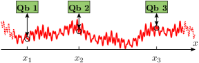
The substrate that supports the qubits also possesses its own degrees of freedom like nuclear spins and phonons. They generally are coupled to the qubits and, thereby, cause quantum dissipation and decoherence.Leggett et al. (1987); Hänggi et al. (1990); Grifoni and Hänggi (1998); Gardiner (1991); Dittrich et al. (1998); Breuer and Petruccione (2002) In experiments, one usually observes both dephasing and relaxation, with dephasing happening on a faster time scale.Borri et al. (2001); Mozyrsky et al. (2002); Muljarov and Zimmermann (2004) It has been noted that the reduced qubit dynamics in principle can be solved exactly if the qubits experience pure phase noise,Luczka (1990); van Kampen (1995); Unruh (1995); Palma et al. (1996); Duan and Guo (1998); Krummheuer et al. (2002); Yu and Eberly (2002, 2003); Solenov et al. (2007) and here we focus on this case as well. In Ref. Doll et al., 2006, we recently presented explicit expressions for the dephasing of two initially entangled qubits. A central conclusion of that work is that the entanglement of a robust entangled stateYu and Eberly (2002); rob is not perfectly stable but undergoes an initial decay, stemming from the spatial qubit separation sketched in Fig. 1. This puts limitations on the applicability of the concept of decoherence-free subspaces, since at best decoherence-poor subspaces emerge instead.
Here we discuss the effects of phase noise on the -qubit generalization of the mentioned robust entangled state, namely the so-called W state,Dür et al. (2000) which is a coherent superposition of all states with exactly one qubit in state while all the others are in state [cf. Eq. (12)]. The W states play an important role in several protocols for quantum information processing, for example quantum teleportation,Joo et al. (2003); Agrawal and Pati (2006) superdense coding Agrawal and Pati (2006) and quantum games.Han et al. (2002) In quantum optics, the W states have already been realized, first with three,Eibl et al. (2004); Roos et al. (2004); Mikami et al. (2005) and recently even with eight qubits.Häffner et al. (2005) Proposals exist to produce W states in atomic gases Gorbachev et al. (2003) and in solid-state environments.Bruss et al. (2005); Saito et al. (2006); Wubs et al. (2007)
In the limit of weak system-bath coupling, a successful and common approach to quantum dissipation is provided by the Bloch-Redfield master equation.Blum (1996) A cornerstone of this formulation is neglecting memory effects of the bath, so that one eventually obtains a Markovian master equation. The indirect interaction of two separated qubits via the environment, however, introduces memory effects that arise when bath distortions can propagate from one qubit to another during a finite time. This timescale can be much larger than the intrinsic memory time of the bath. As will be detailed below, a direct application of the Bloch-Redfield approach to spatially separated qubits predicts spurious decoherence-free subspaces.
In the present work, we pursue a twofold goal: First, we consider an arbitrary number of initially entangled qubits for which we present explicit expressions for the coherence loss. This shows how in a linear arrangement decoherence scales as a function of the number of qubits, and demonstrates the consequences of spatial qubit separations. The stability of the W states with respect to the system size has been studied previously,Carvalho et al. (2004); Simon and Kempe (2002); Dür and Briegel (2004) however for local decoherence models where the qubits couple to effectively independent heat baths. Second, by making a weak-coupling approximation, we derive a non-Markovian master equation approach that captures the main effects of the spatial separation. This approach has the advantage of being more intuitive, while still allowing algebraic methodsLidar et al. (1998); Lidar and Whaley (2003) to be applied to the problem of decoherence. A comparison of the master-equation dynamics and the exact dynamics therefore enables a better interpretation of the latter and a critical examination of the validity of the former. Moreover, the master-equation approach will be applicable as well to other problems that do not possess an exact solution.
The paper is organized as follows: In Sec. II, we present our model, a system of qubits in a linear arrangement. The qubits interact with a thermal bosonic field which causes decoherence of the -qubit state. In Sec. III, we present for pure dephasing the exact time evolution of the concurrence for two qubits initially prepared in a robust entangled Bell-state and then generalize our results to W states of an arbitrary number of qubits. Starting from the general model, we derive in Sec. IV a master equation for the reduced dynamics, taking special care of the spatial qubit separation. Its solution is then compared with the exact results for pure dephasing. The derivations of the exact solution and of a convolutionless master equation are deferred to two appendices.
II Qubits coupled to a bosonic field
As a model for the qubits in the bosonic environment sketched in Fig. 1, we employ the Hamiltonian
| (1) |
where the qubits and the bosonic field in the absence of the coupling are described by the HamiltonianLeggett et al. (1987); Hänggi et al. (1990); Grifoni and Hänggi (1998)
| (2) |
The first term in Eq. (2) represents qubits with energy splittings and Pauli matrices . Since we will not address the coherent control of individual qubits explicitly, the specific choice for the energy splittings is not of major relevance. Note that there is no direct interaction between the qubits. The second term in Eq. (2) describes a bosonic field that consists of modes with energies and the usual bosonic annihilation and creation operators and . We restrict ourselves to a linear dispersion relation with being the sound velocity.
Qubit is located at position and couples linearly via the operator to the field, so that the coupling Hamiltonian reads
| (3) |
with
| (4) |
the bosonic field operator at position . We assume the coupling strengths to be real, isotropic, and identical for all qubits, i.e. and .
We choose an initial condition of the Feynman-Vernon type, i.e. at time , the bath is at equilibrium and is not correlated with the qubits. Thus the total initial density matrix is a direct product of a qubit and bath density operator,
| (5) |
Here, is the reduced density matrix of the qubits and
| (6) |
is the canonical ensemble of the bosons at temperature and is the corresponding partition function.
The dynamics of the qubits plus the environment is governed by the Liouville-von Neumann equation
| (7) |
The tilde denotes the interaction-picture representation with respect to , i.e. , where . We are exclusively interested in the state of the qubits, so our goal is to find the time evolution of the reduced density operator , where denotes the trace over the environmental degrees of freedom. In what follows, we will consider the density matrix elements in the basis , where and .
III Exact reduced dynamics
Generally, the coupling of a qubit to an environment induces spin flips and also randomizes the relative phase between the eigenstates of the qubit. If the coupling operator commutes with the qubit Hamiltonian, the qubits experience the so-called pure phase noise. Consequently, one finds so that the interaction-picture qubit operators remain time-independent, . In particular, the time-evolution of the reduced density operator is independent of the coherent oscillation frequencies of the qubits.
In the following, we consider the coupling operators which constitute a case of pure phase noise. The reduced qubit dynamics can then be solved analytically. We defer the explicit derivation to Appendix A, where we obtain
| (8) |
with the amplitude dampingmis
| (9) |
and the time-dependent phase shift
| (10) |
For ease of notation, we have set the initial time and introduced the bath spectral density . The transit time of a wave between the qubits and reads , where . We will focus on a linear arrangement of the qubits and consider equal nearest-neighbor separations . Then the transit time becomes .
To elaborate on the impact of spatially correlated noise, we assume the chain of qubits to be embedded in a medium with a channel structure, i.e. we treat the bosonic field as effectively one-dimensional. Quasi one-dimensional geometries may, for example, be realized by carbon nanotubes or linear ion traps. They represent configurations in which the requirements of qubit protection and adressability are well-balanced, and where we expect the effects of spatial noise correlations to be most overt. In this case, the spectral density is of the ohmic type,Leggett et al. (1987)
| (11) |
wherein denotes a cutoff frequency which for a phonon field is the Debye frequency. For a more detailed discussion on the relation of the spectral density to the substrate geometry, in particular in the context of semiconductor quantum dots, we refer the reader to Refs. Fedichkin and Privman, 2007; Solenov et al., 2007.
For a physical realization with a GaAs substrate, the Debye frequency is of the order while the sound velocity is . Then a qubit separation corresponds to the transit time . Likewise, for a temperature we have . This implies that is typically the smallest timescale of the problem, while the transit time and the thermal coherence time can be of the same order. The present work is devoted to the effects of spatial separation between qubits, but not of the finite extent of the qubits themselves. Note that in semiconductor quantum dots, the finite width of an electron wavefunction in the dot (typically below 100 nanometers) may lead to an effective cutoff frequency that is smaller than the Debye frequency, but still larger than all other frequencies in the system.Brandes and Vorrath (2002); Fedichkin and Fedorov (2004); Vorojtsov et al. (2005)
Both the damping (9) and the phases (10) vanish at time , so that Eq. (8) is consistent with the initial condition. As expected for pure dephasing, populations are preserved, i.e. the diagonal matrix elements obey . This implies that generally neither the qubits nor the total system will reach thermal equilibrium. However, the relative phases between eigenstates will be randomized so that off-diagonal density matrix elements — the so-called coherences — may decay, which reflects the process of decoherence.
III.1 Dephasing of robust entangled states
A most relevant decoherence effect in a quantum computer is the loss of entanglement between different qubits. In order to exemplify the impact of a spatial qubit separation on decoherence, we consider as the initial state the robust entangled -qubit W state
| (12) |
For two qubits () it has been shown that the two-qubit entanglement inherent in the state , which is the symmetric Bell state, is robust under dephasing for vanishing spatial separation,Yu and Eberly (2002, 2003) while it decays for finite separation. Palma et al. (1996); Doll et al. (2006)
Our motivation to focus on the initial states (12) is twofold: First, W states play an important role in several protocols for quantum information processing,Joo et al. (2003); Han et al. (2002); Agrawal and Pati (2006) so that their sensitivity to an environment is relevant in itself. Second, among all fully entangled -qubit states the states are special in that they maintain their -qubit entanglement under collective dephasing (i.e. for vanishing qubit separations). Now if already the W states start to loose their entanglement due to a finite spatial separation of the qubits, then this is a strong indication that for other fully entangled -qubit states, the situation would be worse. Or, to put it simply, we wish to give the most optimistic estimate about -qubit decoherence and to our knowledge the best way to do that is by focusing on the W states.
The fact that no bit flips occur under pure dephasing is reflected in the structure of the exact solution (8): All density matrix elements that are initially zero remain zero, so that for the state , the dissipative quantum dynamics is restricted to the states
| (13) |
Thus at most out of density matrix elements are nonvanishing. Initially they are all equal, i.e. . From the Hamiltonian (2) it directly follows, that the states possess the eigenenergies and a back-transformation of the coherence to the Schrödinger picture provides the phase factor .
Frequency shifts.
One effect of the coupling to a heat bath is a frequency shift which we obtain in the following way: Upon noticing that one can separate the phases (10) into terms that depend on only or , we write . Each turns out to consist of a finite contribution and a contribution that grows linearly in time, i.e. . The latter leads to a (static) frequency shift. For the ohmic spectral density (11), we obtain
| (14) | ||||
| (15) |
Thus the effective energy splitting of qubit becomes . Note that both and depend on the transit times and the system size but not on the temperature. They can be interpreted as a result from an effective coherent interaction of the qubits mediated by the vacuum fluctuations of the bosonic field,Solenov et al. (2007) where arises from an induced static exchange interaction and its onset is described by . Note that the dominant contribution to the static shift stems from the diagonal terms in Eq. (14), whereas the non-diagonal terms are suppressed by a factor , respectively.
We henceforth work in the interaction picture with respect to the renormalized energies so that the density matrix element reads
| (16) |
The time-dependent phases decay to zero after a rather short time and, thus, influence the decoherence process only during a short initial stage.
Damping factors.
The coherence loss is given by the damping factors . Inserting the ohmic spectral density (11) into expression (9), we obtain for them the explicit form
| (17) |
where denotes the Euler Gamma function. The nominator of the second factor in Eq. (17) itself is already of physical interest: It describes the decoherence of a single qubit in the absence of the other qubits.Doll et al. (2006) One can identify three stages in the single-qubit time evolution:Palma et al. (1996) Very shortly after the preparation, i.e. for times , the fluctuations of the bosonic field are not yet effective, leading to a “quiet regime” in which essentially no single-qubit decoherence takes place. At an intermediate stage, , the main origin of single-qubit decoherence is vacuum quantum fluctuations. They lead to an initial slip of the coherence which we discuss in detail below. Finally for times larger than the thermal coherence time, , thermal fluctuations dominate the coherence loss. The dephasing will finally be complete, i.e. a single qubit that starts in a superposition will loose all quantum coherence due to dephasing caused by the one-dimensional bath.Doll et al. (2006)
For the spatially separated qubits prepared in the W state (12) that we focus on here, the transit times introduce additional time scales after which the denominator of the second factor in Eq. (17) becomes relevant. Since the denominator ultimately decays equally fast as the nominator, decoherence will come to a standstill. This interesting behavior does not occur for a single qubit and will now first be investigated for the case of a qubit pair.
III.2 Entanglement of qubit pairs
It is instructive to first consider the case of two qubits, , which represents the most basic system in which a spatial qubit separation influences quantum coherence. The robust initial state (12) then reduces to the maximally entangled Bell state
| (18) |
where the last expression refers to the basis (13).
For a bipartite system, the degree of entanglement can be measured by the concurrenceWootters (1998)
| (19) |
where the denote the eigenvalues of the matrix in decreasing order and is the complex conjugate of . For qubit pairs that are initially prepared in state (18) and subject to pure phase noise, the concurrence can be expressed at all times by the absolute value of a single non-diagonal element, namely , irrespective of the spatial separation.Doll et al. (2006)
Figure 2 shows the time dependence of the concurrence of a qubit pair prepared in the robust entangled state (18) for various spatial separations. For vanishing separation, we find the concurrence , which means that the entanglement indeed remains perfect and justifies the designation “robust entangled state”.Yu and Eberly (2002, 2003) This is tantamount to saying that the state is an element of a so-called decoherence-free subspace of the two-qubit Hilbert space. However, Fig. 2 also shows that the concurrence of the robust state does decay if the qubit separation is finite. The decay lasts until the transit time is reached. From then on, the concurrence remains constant, so that both the entanglement and the coherence become stable. Thus, we can conclude that for spatially separated qubits the state is not an element of a decoherence-free subspace, but rather of a decoherence-poor subspace. Its emergence from the exact solution (17) will be discussed for the more general case of qubits in the subsequent section. Moreover, a more intuitive picture will be drawn in the framework of a causal master equation approach in Sec. IV.
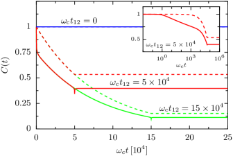
Further information is provided by the value to which the concurrence saturates. Figure 2 shows that is influenced by both the transit time between the qubits and the properties of the bosonic field. The exact value can be obtained from Eq. (17) and reads
| (20) |
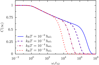
Figure 3 shows this final concurrence as a function of the transit time for various temperatures . As for the time-evolution, three regimes can be identified: For the (unphysically small) separations , the concurrence remains at , while for , the entanglement is no longer perfect, but still at an appreciably large value. For large separations, , the concurrence essentially decays to zero. The latter limit is a prerequisite for the application of quantum error-correction schemes that assume that the qubits experience uncorrelated noise.
Summarizing our two-qubit results, we find that the two-qubit concurrence can saturate at a stable value as long as the separation of the qubits stays finite, i.e. as long as . Remarkably, the coherence of a single qubit in the same environment (i.e. when only one qubit is present) decays completely. The entanglement dynamics that we find for the robust-entangled Bell state (18) is highly non-Markovian and it is obvious that such a behavior can not be described by a Markovian master equation such as the standard Bloch-Redfield equations, as we discuss below. This fact, and in particular the final saturation of concurrence as shown in Figs. 2 and 3 contradict expectations formulated in Ref. Solenov et al., 2007; calculations in that work involve non-entangled initial states, while we study robust-entangled Bell states.
Finally, we want to note that an entanglement saturation under pure dephasing may appear for baths with super-ohmic spectral densities as well,Krummheuer et al. (2002); Roszak and Machnikowski (2006); Doll et al. (2006) even in the limit of large qubit separations. This behavior is in contrast to the intuition emerging from recent work,Yu and Eberly (2002, 2003) namely that the entanglement would always decay to zero when qubits are coupled to independent heat baths. For super-ohmic baths in higher dimensions, a finite final entanglement does not necessarily stem from spatial correlations. This becomes obvious from the fact that for super-ohmic baths as for example a three-dimensional phonon field, the coherence of single qubits exhibits a similar saturation.
III.3 -qubit fidelity
Let us now turn to the intriguing question how the previous results can be generalized to arrays of qubits. As already described above, the focus will be on the scaling of the decoherence as a function of the system size of linearly arranged qubits. In particular, we study how the amount of entanglement evolves for the qubits that start in the -qubit W state (12) and, due to dephasing, at later times must be described by the -qubit density matrix (8).
With the exact dynamics known, the only remaining question is how to quantify the entanglement. If there were no interaction with the environment, then the qubits would remain in their pure entangled W state (12), which in density-matrix notation reads . After the dissipative time evolution, the qubit state deviates from this “ideal” output state . The question is how much. A proper measure for this quantity is the fidelityPoyatos et al. (1997) , which in our case reads
| (21) |
In general, the fidelity is bounded by , where corresponds to a pure state.Nielsen and Chuang (2000) For qubits subject to pure dephasing, the somewhat more strict condition applies, because the populations do not change. In particular the inequalities will hold for the initial state , as illustrated below. To give another argument why fidelity makes a good measure of entanglement for our particular purpose, we emphasize that for two qubits prepared in the state (18), the fidelity directly relates to the concurrence via the relation .
We note in passing that for other initial states that are not pure -qubit entangled states, one should be careful to use fidelity as an entanglement measure, for example because the fidelity may remain constant while the system undergoes nontrivial dynamics.Fedichkin and Privman (2007) Finding other entanglement measures for three or more qubits is an active field of research.Dür et al. (2000); Mintert et al. (2005); Lohmayer et al. (2006); Horodecki et al. (2007) Their numerical evaluation can be rather involved, especially for larger systems. These issues need not concern us here, since we start with an -qubit entangled pure state for which the fidelity is a good measure of entanglement. The fidelity has the additional advantage that it is easily evaluated analytically for larger systems as well.
For the robust state (12), the fidelity becomes
| (22) |
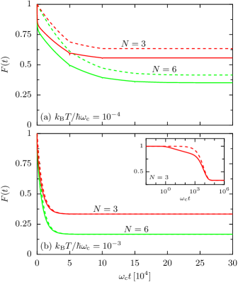
where the coherences are given in Eq. (16). The time evolution of the fidelity for and for qubits is shown in Fig. 4. For low temperatures [panel (a)], we find that the fidelity decay is slowed down whenever a transit time is reached, i.e. at times . This resembles the behavior of the concurrence for two qubits shown in Fig. 2. For a larger number of qubits, the fidelity saturates at a lower value.
In order to gain a more quantitative understanding of the fidelity saturation, we focus on the final fidelity . In the zero-temperature limit, which provides a lower bound for the coherence loss, we find from Eqs. (16) and (17) the density matrix elements . Hence the fidelity (22) saturates to
| (23) |
Although we start out with a “robust” entangled state, this final fidelity can be as low as , which marks the large-distance limit . More generally, we find that for zero temperature, the final fidelity decreases with increasing cutoff frequency , increasing spatial separation, and for a larger qubit-bath coupling strength .
An intriguing aspect of the fidelity is its scaling behavior as a function of the system size . Will decay to zero for larger arrays of qubits, or converge to a finite value? For large we can neglect the term in Eq. (23) and replace the sum over by an integration over the continuous variable . Then we obtain
| (24) | |||||
where the evaluation of the integral yields Gauss’ hypergeometric function . The expression (24) is valid for general coupling constant , but beyond weak coupling its value is rather small. We will now approximate Eq. (24) for . Furthermore, usually many cutoff wavelengths will fit between two neighboring qubits, so that , as we argued above. Since we already assumed to arrive at the integral (24), we are surely in the limit . Then we can approximate the hypergeometric function by its asymptotic expansion for large fourth argument. We finally obtain
| (25) |
Hereby we found the important result that although the final fidelity is smaller for larger systems, the scaling is only algebraic in . This stability under dephasing is a property of the initial -qubit W state (12). Clearly, for nonvanising this state lives in a decoherence-poor rather than in a decoherence-free subspace. Equation (25) shows that at zero temperature, the final fidelity is determined by two dimensionless numbers, the one number being and the other the ratio between the array length and the cutoff wavelength .
In Fig. 5, we compare for two values of the exact expression (23) for the final fidelity as a function of with the weak-coupling approximate result (25). Clearly, for state-of-the-art well-isolated qubits with typically , the agreement is excellent already for , while for convergence is reached for . The figure clearly shows that in the weak coupling limit , the final fidelity in (25) is almost independent of the length of the array. For the factor in square brackets in Eq. (25) is less than , so that the large- expression for the final fidelity could be further simplified as .
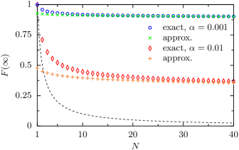
The above estimates were derived in the limit of strictly zero temperature, so that the question arises up to which temperature they still represent a reasonably good approximation. A closer inspection of the exact result (17) reveals that this is certainly the case if the condition
| (26) |
holds, i.e. if the thermal coherence length of the bath is much larger than the length of the array. Assuming , the thermal coherence length is . This value corresponds to an array length of qubits with a nearest-neighbor distance . The final fidelity that we obtain for in Eq. (25) can therefore be considered as an upper bound for what could be realized in state-of-the-art quantum information processing experiments on arrays of qubits.
IV Causal master equation
In Sec. III, we found that the analytical solution for the qubit dynamics can involve rather complex expressions and, thus, an intuitive picture of the observed behavior can be hard to find, even though the exact solution is known. Thus for a more qualitative understanding, one can benefit from an approximative treatment in the spirit of a Bloch-Redfield master equation approach. Moreover, such an approach enables a symmetry analysis of the dissipative time evolution. This can provide additional insight in cases in which tracing out the bath degrees of freedom reveals symmetries that are obeyed by the dissipative central system, but not by the system-bath Hamiltonian.
Bloch-Redfield equations are based on a perturbative treatment of the qubit-environment coupling, followed by neglecting memory effects in the kernel of the resulting quantum master equation. Thereby one entirely ignores the dependence of the dynamical equations on the qubits’ history and, thus, on the initial preparation. The resulting master equation then assumes the structure . Such equations, however, fail to reproduce the stepwise decay of the concurrence observed in Sec. III. For the concurrence of the robust Bell state (18), they even yield for all distances , in clear contrast to the exact solution. In other words, strictly Markovian master equations can predict spurious decoherence-free subspaces. In this section, we shall derive a master equation that does not suffer from such a shortcoming.
IV.1 Markov approximation and beyond
Taking the above considerations as a motivation, we now derive a generalization of the Bloch-Redfield master equation that is able to capture the retardation effects stemming from a finite sound velocity. In doing so we pursue closely the standard approach that leads to a Markovian equation of motion. In this way, it can be identified where it fails and how to improve it accordingly.
Starting with the Liouville-von Neumann equation (7), we employ a projection-operator formalism to formally eliminate the bath degrees of freedom. In second-order perturbation in the qubit-bath coupling, we obtain for the reduced qubit density matrix the master equation
| (27) |
where and the super-operator
| (28) |
with the anti-commutator . For a sketch of the derivation, see Appendix B. Although this master equation is in a time-convolutionless form, it still is non-Markovian owing to the explicit dependence on the initial time . The integral kernel (28) features the real part and the imaginary part of the bath correlation function . For our bath model they can be evaluated explicitly and read
| (29) | ||||
| (30) |
where
| (31) | ||||
| (32) |
are the usual symmetric and anti-symmetric bath correlation functions,Leggett et al. (1987); van Kampen (2001); Breuer and Petruccione (2002) respectively.
We first consider the local terms, i.e. those with , for which the time shift vanishes. Then the correlation functions (29) and (30) reduce to Eqs. (31) and (32), respectively, and one can introduce a Markov approximation in the usual way: If the correlation functions and contribute to the integral in Eq. (27) essentially in a small time interval of size around , then for , we can extend the -integration to infinity, i.e. we set
| (33) |
This expression implies a coarse-graining in time so that the resulting master equation is valid only for time steps not smaller than the bath correlation time . In general, the bath correlation time depends on the properties of the spectral density and the temperature of the bath. If the temperature is not too low and the spectral density is fairly smooth and decays sufficiently fast for and , as is the case here, then the correlation time is only weakly temperature dependent and reads .Cheng and Silbey (2005)
In the above treatment of the local terms , we have followed the route towards a Markovian equation of motion. For the nonlocal terms, however, the arguments of the last paragraph are no longer valid. For the correlation functions (29) and (30) are not peaked at , but at which for a realistic qubit separation typically exceeds the bath correlation time . Then we have to distinguish the cases and . In the former case, the peak of the correlation functions lies outside the integration interval so that the integral is small and, consequently, will be neglected. In the latter case, by contrast, the peak fully contributes so that the integral can again be extended to infinity. In summary, this means
| (34) |
where is the Heaviside step function. For , this expression coincides with Eq. (33).
Inserting the approximation (34) into the weak-coupling master equation (27) and setting again the initial time , we find the causal master equation (CME)
| (35) |
with the time-dependent superoperator
| (36) |
The step functions ensure causality which requires that the cross terms can only be active after the propagation time between the respective qubits has passed. In the limit of vanishing separation, the causal master equation reduces to a standard Bloch-Redfield equation. In the following, we will demonstrate that the causal master equation reproduces the results of Sec. III rather well, while a standard Bloch-Redfield approach clearly fails.
IV.2 Master equation for pure dephasing
Let us now apply the causal master equation to the problem defined in Sec. II and test the results against the exact solutions presented in Sec. III. Since commutes with the free Hamiltonian , the interaction-picture coupling operators stay time-independent, . Then the time integration in the causal Bloch-Redfield tensor (36) involves only the bath correlation functions and we obtain for the density matrix element the equations of motion
| (37) |
with the damping
| (38) | ||||
| and the phase shift | ||||
| (39) | ||||
This master equation is non-Markovian due to the appearance of the step functions, which change the effective damping and phase shift whenever a transit time is reached. These stepwise time-dependent frequency shifts and decay rates are characteristic features of the causal master equation. As we will see, because of these steps the CME follows more closely the smooth time-dependent variations of shifts and decay rates of the exact dynamics than the standard master-equation formalism manages to do with its static shifts and decay rates.
As in Sec. III, we first consider as an initial state the robust Bell state (18). From the master equation (37), we find that the concurrence obeys
| (40) |
This differential equation is readily integrated to provide the solution
| (41) |
i.e. the concurrence decays exponentially until the transition time is reached and thereafter remains constant. This clear separation of two dynamical regimes facilitates an intuitive interpretation: For times , the qubits have not “seen” each other, so that we are in a regime of single-qubit decoherence. Indeed, during this first time interval the causal master equation (37) coincides with a standard Bloch-Redfield approach in which the qubits are coupled to independent heat baths. Consequently, the relative phase between the qubits is randomized and the concurrence decays. However, for , both qubits experience correlated quantum noise and undergo collective decoherence. Thus, the concurrence decay comes to a standstill and a decoherence-poor subspace can emerge.
This time evolution is compared to the exact solutions in Fig. 2. We find that generally the causal master equation describes the slow decay of the concurrence and its saturation very well. At very short times, however, the causal master equation does not capture the initial slip of the concurrence. The reason for this is, that the dynamics on timescales that are comparable to the bath correlation time cannot be resolved in a coarse-grained time approximation underlying the causal master equation. The same generally holds true for Markovian quantum master equations, in particular for the standard Bloch-Redfield equation. At larger times, the benefits of the causal master equation become obvious: Since the Bloch-Redfield treatment is recovered by setting the transit time , Eq. (40) reveals that for all times, i.e. the concurrence remains at its initial value. This spurious robustness of the concurrence is, however, in clear contrast to the exact result. For pure phase noise, the populations of the system eigenstates are conserved and, consequently, the final state is generally unrelated to thermal equilibrium. Therefore, the question whether the master equation can describe the grand canonical ensemble of the system coupled to the bath is in the present context ill-posed.
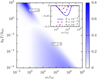
For a quantitative investigation of the quality of the causal master equation, we compare the final values of the concurrence, . Figure 6 depicts the difference of the exact solution and the causal master equation result, , as a function of transit time and temperature. For realistic temperatures , Fig. 6 shows that the final value obtained from the causal master equation exceeds the exact result, so that provides an upper bound for the concurrence. In particular, for , the agreement is almost perfect. Note that for very high temperatures , the difference assumes also positive values.
Let us finally apply the master equation (37) also to the case of a linear -qubit arrangement with equal nearest-neighbor spacings as discussed in Sec. III.3. We again consider the initial preparation in the robust state (12) using the shorthand notation (13). To calculate the fidelity defined in Eq. (22), we need to compute the values of the density matrix elements . Unlike for the two-qubit concurrence, phase shifts now also play a role. The time-dependent phase shift [see Eq. (39)] can be written as the difference of two terms, the one only depending on and the other only on . Both terms describe stepwise time-dependent frequency shifts of the corresponding qubits. Interestingly, after the longest transit time , these shifts in the CME become static and agrees with the exact result (14), i.e. . For an unambiguous comparison of fidelities in the exact and in the causal master-equation formalism, it is an important result that we can work in the same interaction picture with the same renormalized frequencies . It remains to be discussed what is the effect of the stepwise frequency shifts in the CME for times . It is the non-diagonal terms in Eq. (39) that make up the difference between the frequency shifts at time and the exact static renormalization at times . However, this difference is very small due to large factors in the denominator of Eq. (39), and can safely be neglected in the following.
From the causal master equation (37) we then obtain
| (42) |
Interestingly enough, in the present case only two types of terms of the master equation (37) contribute: the local terms with and those with . As a consequence, the decay rate of changes only at the transit time .
In order to evaluate the fidelity (22), we integrate Eq. (42) and sum over all density matrix elements , so that we obtain
| (43) |
For vanishing qubit separation, the master equation predicts , i.e. a decoherence-free behavior. For , however, all coherences initially decay and so does the fidelity. When the smallest transit time is reached, a perfect correlation between nearest neighbors is built up and the coherences saturate. Since these coherences are no longer time-dependent, the fidelity decay is reduced accordingly. This process continues until ultimately all transition times have passed, i.e. until , and the fidelity decay comes to a standstill.
In Fig. 4, we compare this behavior to the exact solution. For very low temperatures [panel (a)], we observe that the master equation reproduces the reduction of the fidelity decay whenever a transit time is reached. The relative difference between the exact result and the causal master equation is of the order of 10% as in the case of two qubits. If the temperature becomes larger, so that the nearest neighbor separation exceeds the thermal coherence length [see Fig. 3 and the discussion after Eq. (20)], then the fidelity decay is determined by thermal noise. In that case, already saturates to a rather small value before the first transit time is reached. The inset of Fig. 4b shows that at very short times when the decay sets in, i.e. when the CME is not yet different from a standard master equation for independently dephasing qubits, that then the CME result can deviate significantly from the exact result. Again we wish to stress that this deviation is due to the coarse-grained time approximation that is inherent in a standard master equation approach as well. However, in contrast to the latter, the CME and the exact results agree very well at later times.
V Discussion and conclusions
Decoherence of an array of qubits can be a rather complex process that proceeds in several qualitative different stages, even in the case of pure phase noise which we investigated here: If the qubits are coupled to the bosonic field of the substrate vibrations, the dynamics during a first, very short period is essentially noiseless. In a second stage, the bosonic vacuum fluctuations are most relevant, while finally, thermal noise dominates. The spatial separation of the qubits brings in further time scales, namely the transit times of sound waves between the qubits.
Here we considered robust entangled -qubit W states, which do not decohere for vanishing qubit separations. For finite separations we find instead that the qubits start to dephase. However, the dephasing slows down whenever the elapsed time reaches a transit time, until it eventually comes to a standstill. The final -qubit quantum coherence increases with decreasing qubit-qubit separation, qubit-bath coupling strength, cutoff frequency, and temperature. By contrast, single qubits in the same one-dimensional environment would loose all quantum coherence for all finite values of these bath parameters. Note that, the two-qubit W state is identical to the robust-entangled Bell state. The saturation of entanglement that we find does not occur for fragile two-qubit states.Doll et al. (2006); Solenov et al. (2007)
Cooperative effects can be advantageous or detrimental, depending on the specific protocol that one has in mind. For example, one may fight decoherence by creating decoherence-free subspaces. To that end, one could bring the qubits close together and use the W states for quantum information processing because their entanglement is robust. Nevertheless, the qubits must be sufficiently well separated, either to enable their individual manipulation or because of their finite extensions. We found that this requirement prevents the realization of decoherence-free subspaces. Cooperative effects are still advantageous, since decoherence-poor subspaces are built up instead. Good results require the length of the array of qubits to be smaller than the thermal coherence length .
Alternatively, one may wish to implement active quantum error-correction schemes, where logical qubits are redundantly encoded into several physical qubits. Here, by contrast, the cooperative effects are detrimental, since standard error-correction schemesNielsen and Chuang (2000); Klesse and Frank (2005) and recent generalizations to non-Markovian bathsTerhal and Burkard (2005); Aliferis et al. (2006) will only work perfectly if the physical qubits couple to spatially uncorrelated baths. Our discussion demonstrates that neighboring physical qubits should then be separated by more than the thermal coherence length . By reducing the temperature, single-qubit dephasing is suppressed, but the assumption of uncorrelated baths becomes worse. This suggests that there may be an optimal working temperature for quantum error correction, given a geometry of physical qubits.
Thus our calculations show how well decoherence-free subspaces or quantum error correction-protocols could be realized with linear arrays of qubits. The aforementioned conflicting requirements for both strategies seem to rule out the implementation of both strategies in one experiment.
One should keep in mind that bit-flip noise, which was not considered here, will reduce coherence further, although typically on a longer time scale. Including bit-flip noise usually renders the qubits-environment model no longer exactly solvable. Therefore one has to resort to approximation schemes like, e.g, a master-equation approach. As we have shown, the common Bloch-Redfield master equation cannot account for the intrinsically non-Markovian effects stemming from the spatial separations. For the present model, the Bloch-Redfield approach predicts spurious decoherence-free subspaces, which in fact are at best decoherence-poor. Very recently, it was foundKarasik et al. (2007) that for bit-flip noise due to a homogeneous isotropic Markovian and three-dimensional reservoir, there is no multi-particle decoherence-free subspace outside the Dicke limit, i.e. whenever the qubits are not co-located. The situation may be different for one-dimensional structures for which we find that at least for pure dephasing, decoherence-free subspaces can become imperfect if the qubits are separated.
In order to capture delocalization effects with a master equation, we have derived a modified Bloch-Redfield approach that ensures causality for the qubit-qubit interaction mediated by the substrate. It proved to be reliable for parameters for which the standard master equation for a single qubit is reliable. This is the case for sufficiently high temperatures or small enough coupling strengths such that initial-slip effects are small. A characteristic feature of the proposed causal master equation is that it selects the Bloch-Redfield kernel depending on the time elapsed since the preparation. This means that the time evolution is governed by a time-dependent Liouville operator which renders the dynamics non-Markovian. Besides being a proper tool for studying retardation effects in models that do not possess an exact solution, the causal master equation describes the time evolution in an intuitive and concise manner. Thereby, it enables decoherence studies with algebraic methods which possibly will provide suggestions for coherence stabilization.
In this sense, our studies of the interplay between pure dephasing and a spatial qubit separation can only be a first step towards a deeper understanding of such phenomena. In particular the inclusion of other quantum noise sources, which are also present in real experiments, will complement the picture drawn above.
Acknowledgements.
This work was supported by Deutsche Forschungsgemeinschaft through SFB 484 and SFB 631. PH and SK acknowledge funding by the DFG excellence cluster “Nanosystems Initiative Munich”.Appendix A Exact reduced dynamics
In this appendix, we outline the derivation of the exact solution (8) for the reduced qubit dynamics for the case of pure dephasing.Palma et al. (1996); Duan and Guo (1998); Reina et al. (2002); Doll et al. (2006). In the usual interaction picture with respect to the uncoupled qubits and the bath, the coupling Hamiltonian (3) reads
| (44) |
with the interaction
| (45) |
Our aim is to calculate the time evolution of the reduced density matrix generated by the propagator
| (46) |
where denotes the time-ordering operator. In a first step, we find , where
| (47) |
Since and for all times and , we can use the Baker-Campbell-Hausdorff formulaGardiner (1991) to express the time-ordered exponential (46) as
| (48) |
The first term in the exponent can be written as
| (49) |
where we defined and the displacement operators . The second term in the exponent is a c-number and provides the time-dependent phase factor with
| (50) |
So far we have found for the propagator the expression
| (51) |
For the factorizing initial condition , the matrix elements of the reduced density operator become
| (52) |
In the second equality of Eq. (52) we have used the cyclic property of the trace and the fact that the computational basis elements are eigenstates of the propagator. Inserting the propagator (51) into (52) and assuming an isotropic coupling , we find for density matrix element the phase
| (53) | ||||
| (54) | ||||
which in the continuum limit becomes the phase (10). For the calculation of the remaining contributions in (52), we employ the relations and
| (55) |
which hold for any commuting operators and . Then we obtain
| (56) | ||||
| (57) | ||||
An additional phase stems from the commutator of the displacement operators in (A) [see Eq. (55)] and reads
| (58) |
and vanishes for isotropic coupling which we assume herein.
Finally, we have to evaluate the trace in Eq. (57). This can be accomplished conveniently in the basis of the coherent states , in which the equilibrium bath density operator (6) reads
| (59) |
The integration is over the whole complex plane and is the Bose distribution function. are the complex eigenvalues of the annihilation operator , i.e. . After inserting expression (59) into Eq. (57), we integrate for each mode over the complex plane. We finally end up with
| (60) |
where
| (61) |
Note that is real-valued and thus accounts for the damping of the matrix element. In the continuum limit, it assumes the form (9).
Appendix B Weak-coupling master equation
For notational convenience, we write the Liouville-von Neumann equation (7) with the super-operator , so that it reads , where will serve as an expansion parameter. The formal solution can be written as , where
| (62) |
Moreover, we introduce the projection operator
| (63) |
which projects an operator of the full Hilbert space (of the qubits and the bath) to a direct product of a system operator and a time-independent reference state of the bath. Here, we are interested in the relevant part of the density matrix, which describes the reduced dynamics. The projection operator (63) is constructed such that the factorizing initial condition (5) provides the identity . This allows one to write the formal solution of the dissipative system dynamics in the form
| (64) |
From Eq. (64), one can derive a formally exact quantum master equation for in two ways: The first possibility is the Nakajima-Zwanzig projector techniqueNakajima (1958); Zwanzig (1960) which leads to an integro-differential equation for which is nonlocal in time. The second possibility, on which we will focus here, is termed “time convolutionless projection operator technique”Kubo (1962); van Kampen (1974); Breuer and Petruccione (2002) and leads to a equation of motion of the form
| (65) |
which is local in time, but is governed by an explicitly time-dependent super-operator . Although this equation possesses an apparently simple form, it generally cannot be solved exactly and, thus, one has to resort to a perturbative treatment. In doing so, we expand the generator in powers of the qubit-bath coupling parameter , i.e. . Then a formal integration of Eq. (65) results in
| (66) |
Comparing the powers of of Eqs. (64) and (66), we find the relations
| (67) | ||||
| (68) |
so that the master equation reads
| (69) |
By inserting the definitions of the projection operator (63) and the Liouvillian , we obtain Eq. (27). Note that the coupling (3) results in .
References
- Nakamura et al. (1999) Y. Nakamura, Y. A. Pashkin, and J. S. Tsai, Nature (London) 398, 786 (1999).
- Vion et al. (2002) D. Vion, A. Aassime, A. Cottet, P. Joyez, H. Pothier, C. Urbina, D. Esteve, and M. H. Devoret, Science 296, 886 (2002).
- Chiorescu et al. (2003) I. Chiorescu, Y. Nakamura, C. J. P. Harmans, and J. E. Mooij, Science 299, 1869 (2003).
- Yamamoto et al. (2003) T. Yamamoto, Y. A. Pashkin, O. Astafiev, Y. Nakamura, and J. S. Tsai, Nature (London) 425, 941 (2003).
- Palma et al. (1996) G. M. Palma, K.-A. Suominen, and A. K. Ekert, Proc. R. Soc. London, Ser. A 452, 567 (1996).
- Zanardi and Rasetti (1997) P. Zanardi and M. Rasetti, Phys. Rev. Lett. 79, 3306 (1997).
- Lidar et al. (1998) D. A. Lidar, I. L. Chuang, and K. B. Whaley, Phys. Rev. Lett. 81, 2594 (1998).
- Lidar and Whaley (2003) D. A. Lidar and K. B. Whaley, in Irreversible Quantum Dynamics, edited by F. Benatti and R. Floreanini (Springer, Berlin, 2003), pp. 83–120.
- Leggett et al. (1987) A. J. Leggett, S. Chakravarty, A. T. Dorsey, M. P. A. Fisher, A. Garg, and W. Zwerger, Rev. Mod. Phys. 59, 1 (1987).
- Hänggi et al. (1990) P. Hänggi, P. Talkner, and M. Borkovec, Rev. Mod. Phys. 62, 251 (1990).
- Grifoni and Hänggi (1998) M. Grifoni and P. Hänggi, Phys. Rep. 304, 229 (1998).
- Gardiner (1991) C. W. Gardiner, Quantum Noise, vol. 56 of Springer Series in Synergetics (Springer, Berlin, 1991).
- Dittrich et al. (1998) T. Dittrich, P. Hänggi, G.-L. Ingold, B. Kramer, G. Schön, and W. Zwerger, Quantum transport and dissipation (Wiley-VCH, Weinheim, 1998).
- Breuer and Petruccione (2002) H.-P. Breuer and F. Petruccione, The theory of open quantum systems (Oxford University Press, Oxford, 2002).
- Borri et al. (2001) P. Borri, W. Langbein, S. Schneider, U. Woggon, R. L. Sellin, D. Ouyang, and D. Bimberg, Phys. Rev. Lett. 87, 157401 (2001).
- Mozyrsky et al. (2002) D. Mozyrsky, S. Kogan, V. N. Gorshkov, and G. P. Berman, Phys. Rev. B 65, 245213 (2002).
- Muljarov and Zimmermann (2004) E. A. Muljarov and R. Zimmermann, Phys. Rev. Lett. 93, 237401 (2004).
- Luczka (1990) J. Luczka, Physica A 167, 919 (1990).
- van Kampen (1995) N. G. van Kampen, J. Stat. Phys. 78, 299 (1995).
- Unruh (1995) W. G. Unruh, Phys. Rev. A 51, 992 (1995).
- Duan and Guo (1998) L.-M. Duan and G.-C. Guo, Quantum Semiclass. Opt. 10, 611 (1998).
- Krummheuer et al. (2002) B. Krummheuer, V. M. Axt, and T. Kuhn, Phys. Rev. B 65, 195313 (2002).
- Yu and Eberly (2002) T. Yu and J. H. Eberly, Phys. Rev. B 66, 193306 (2002).
- Yu and Eberly (2003) T. Yu and J. H. Eberly, Phys. Rev. B 68, 165322 (2003).
- Solenov et al. (2007) D. Solenov, D. Tolkunov, and V. Privman, Phys. Rev. B 75, 035134 (2007).
- Doll et al. (2006) R. Doll, M. Wubs, P. Hänggi, and S. Kohler, Europhys. Lett. 76, 547 (2006).
- Dür et al. (2000) W. Dür, G.Vidal, and J. I. Cirac, Phys. Rev. A 62, 062314 (2000).
- Eibl et al. (2004) M. Eibl, N. Kiesel, M. Bourennane, C. Kurtsiefer, and H. Weinfurter, Phys. Rev. Lett. 92, 077901 (2004).
- Roos et al. (2004) C. F. Roos, M. Riebe, H. Häffner, W. Hänsel, J. Benhelm, G. P. T. Lancaster, C. Becher, F. Schmidt-Kaler, and R. Blatt, Science 304, 1478 (2004).
- Häffner et al. (2005) H. Häffner, W. Hänsel, C. F. Roos, J. Benhelm, D. Check-Al-Kar, M. Chwalla, T. Körber, U. D. Rapol, M. Riebe, P. O. Schmidt, et al., Nature 438, 643 (2005).
- (31) In recent literature,Dür et al. (2000); Eibl et al. (2004); Roos et al. (2004); Häffner et al. (2005) the term “robust entanglement” also has also been used with a different meaning, namely for the entanglement of a -qubit state that becomes a -qubit entangled state after tracing out one qubit.
- Joo et al. (2003) J. Joo, Y.-J. Park, S. Oh, and J. Kim, New J. Phys. 5, 136 (2003).
- Agrawal and Pati (2006) P. Agrawal and A. Pati, Phys. Rev. A 74, 062320 (2006).
- Han et al. (2002) Y.-J. Han, Y.-S. Zhang, and G.-C. Guo, Phys. Lett. A 295, 61 (2002).
- Mikami et al. (2005) H. Mikami, Y. Li, K. Fukuoka, and T. Kobayashi, Phys. Rev. Lett. 95, 150404 (2005).
- Gorbachev et al. (2003) V. N. Gorbachev, A. A. Rodichkina, A. I. Trubilko, and A. I. Zilba, Phys. Lett. A 310, 339 (2003).
- Bruss et al. (2005) D. Bruss, N. Datta, A. Ekert, L. C. Kwek, and C. Macchiavello, Phys. Rev. A 72, 014301 (2005).
- Saito et al. (2006) K. Saito, M. Wubs, S. Kohler, P. Hänggi, and Y. Kayanuma, Europhys. Lett. 76, 22 (2006).
- Wubs et al. (2007) M. Wubs, S. Kohler, and P. Hänggi, Physica E (in press), arXiv:cond-mat/0703425 (2007).
- Blum (1996) K. Blum, Density Matrix Theory and Applications (Plenum Press, New York, 1996), 2nd ed.
- Carvalho et al. (2004) A. R. R. Carvalho, F. Mintert, and A. Buchleitner, Phys. Rev. Lett. 93, 230501 (2004).
- Simon and Kempe (2002) C. Simon and J. Kempe, Phys. Rev. A 65, 052327 (2002).
- Dür and Briegel (2004) W. Dür and H.-J. Briegel, Phys. Rev. Lett. 92, 180403 (2004).
- (44) Note that the expression for in Ref. Doll et al., 2006 contains a misprint. The correct expression is Eq. (9).
- Fedichkin and Privman (2007) L. Fedichkin and V. Privman, in Electron Spin Resonance and Related Phenomena in Low Dimensional Structures, edited by M. Fanciulli (Springer, Berlin, 2007), Topics in Applied Physics, see also arXiv:cond-mat/0610756.
- Brandes and Vorrath (2002) T. Brandes and T. Vorrath, Phys. Rev. B 66, 075341 (2002).
- Fedichkin and Fedorov (2004) L. Fedichkin and A. Fedorov, Phys. Rev. A 69, 032311 (2004).
- Vorojtsov et al. (2005) S. Vorojtsov, E. R. Mucciolo, and H. U. Baranger, Phys. Rev. B 71, 205322 (2005).
- Wootters (1998) W. K. Wootters, Phys. Rev. Lett. 80, 2245 (1998).
- Roszak and Machnikowski (2006) K. Roszak and P. Machnikowski, Phys. Rev. A 73, 022313 (2006).
- Poyatos et al. (1997) J. F. Poyatos, J. I. Cirac, and P. Zoller, Phys. Rev. Lett. 78, 390 (1997).
- Nielsen and Chuang (2000) M. A. Nielsen and I. L. Chuang, Quantum Computing and Quantum Information (Cambridge University Press, Cambridge, 2000).
- Mintert et al. (2005) F. Mintert, A. R. R. Carvalho, M. Kuś, and A. Buchleitner, Phys. Rep. 415, 207 (2005).
- Lohmayer et al. (2006) R. Lohmayer, A. Osterloh, J. Siewert, and A. Uhlmann, Phys. Rev. Lett. 97, 260502 (2006).
- Horodecki et al. (2007) R. Horodecki, P. Horodecki, M. Horodecki, and K. Horodecki, Quantum entanglement, arXiv:quant-ph/0702225 (2007).
- van Kampen (2001) N. G. van Kampen, Stochastic processes in physics and chemistry (North-Holland, Amsterdam, 2001).
- Cheng and Silbey (2005) Y. C. Cheng and R. J. Silbey, J. Phys. Chem. B 109, 21399 (2005).
- Klesse and Frank (2005) R. Klesse and S. Frank, Phys. Rev. Lett. 95, 230503 (2005).
- Terhal and Burkard (2005) B. M. Terhal and G. Burkard, Phys. Rev. A 71, 012336 (2005).
- Aliferis et al. (2006) P. Aliferis, D. Gottesman, and J. Preskill, Quant. Inf. Comput. 6, 97 (2006).
- Karasik et al. (2007) R. I. Karasik, K.-P. Marzlin, B. C. Sanders, and K. B. Whaley, Multi-particle decoherence free subspaces in extended systems, arXiv:quant-ph/0702244 (2007).
- Reina et al. (2002) J. H. Reina, L. Quiroga, and N. F. Johnson, Phys. Rev. A 65, 032326 (2002).
- Nakajima (1958) S. Nakajima, Prog. Theo. Phys. 20, 948 (1958).
- Zwanzig (1960) R. Zwanzig, J. Chem. Phys. 33, 1338 (1960).
- Kubo (1962) R. Kubo, J. Phys. Soc. Jap. 17, 1100 (1962).
- van Kampen (1974) N. G. van Kampen, Physica 74, 215 (1974).