Quantum mechanics of spin transfer in coupled electron-spin chains
Abstract
The manner in which spin-polarized electrons interact with a magnetized thin film is currently described by a semi-classical approach. This in turn provides our present understanding of the spin transfer, or spin torque phenomenon. However, spin is an intrinsically quantum mechanical quantity. Here, we make the first strides towards a fully quantum mechanical description of spin transfer through spin currents interacting with a Heisenberg-coupled spin chain. Because of quantum entanglement, this requires a formalism based on the density matrix approach. Our description illustrates how individual spins in the chain time-evolve as a result of spin transfer.
pacs:
72.10.Bg, 72.25.Ba, 75.10.JmThe problem of switching the spin state of a ferromagnet has its origins in magnetization reversal through an applied magnetic field choi01 . The present understanding of this process is based on the (numerical) solution of the so-called Landau-Lifshitz-Gilbert (LLG) equations mansuripur88 . These equations define a space-dependent magnetization vector, whose magnitude at each spatial coordinate is held fixed, but whose direction is determined by a (classical) dynamical equation which relates the rate of change of magnetization to the applied torque. The applied torque is determined by an effective magnetic field, which represents a mean field as experienced by the magnetization at that particular spatial coordinate. A damping term is also required, which is crucial for the magnetization reversal to take place. A semi-classical approach slonczewski96 ; berger96 was adopted to describe spin transfer myers99 from a spin-polarized current to a ferromagnet. The description of this phenomenon requires a quantum mechanical treatment of the spin current, while a classical notion of the magnetic moment bazaliy98 ; waintal00 ; kim04 suffices for a qualitative understanding of the spin torque process. Most intriguing from our point of view is that a phenomenological damping process is not required for spin torque to occur; in this respect a spin current is profoundly different from an applied magnetic field.
However, more recently, spin transfer has been recognized as important, both in spintronics myers99 ; weber01 ; wolf01 ; kiselev03 ; krivorotov05 ; hirjbehedin06 , and in quantum informationnielsen00 ; leuenberger01 . For these reasons, and because, after all, spin is an intrinsically quantum property, it is critical to understand spin transfer as a fully quantum mechanical process. This way, even within the more conventional applications where the LLG approach has been fairly successful, one can understand and perhaps push the limitations of the semi-classical approach. In this paper we construct the simplest but most important elements of a model with which one can illustrate the spin dynamics quantum mechanically. Consider an electron incident on a ferromagnetic chain with coupled local spins, all prepared magnetized in a particular direction. Unless the electron spin is parallel to the local spins, spin will be transferred to the chain from the electron. In the semi-classical picture, each spin is considered as a classical vector; in particular the magnitude of the vector remains constant, while its direction is allowed to change. On the other hand, within a quantum mechanical description, is an operator avishai01 ; kim05 . It is that remains constant; in contrast, changes during the transfer process, and can even vanish momentarily.
To describe complete spin transfer requires a current of polarized electrons. This introduces another purely quantum mechanical concept associated with spin transfer: entanglement between an electron and the localized spin chain. Even after the electron moves away from the spin chain, the quantum states of the electron and localized spins are entangled in spin space. Thus, to illustrate the dynamics of the chain we should know how to describe a subsystem (spin chain) of a composite system (spin chain and electron). In particular, if we send another electron to interact with the chain after a preceding electron leaves the chain, it is crucial to decouple the spin chain from the first electron quantum mechanically. The density matrix formalism feynman72 is the only way to serve this purpose. Suppose a system consists of two subsystems A and B. This composite system is assumed to be closed. Initially, A and B are separated and no interaction takes place between the two. In other words, A and B are further apart than the interaction range of the two. The quantum states of A and B would be and , respectively. Imagine, now, the two subsystems come together and interact with one another. For example, in our case, the mobile subsystem A (the electron) moves into the region of interaction with the stationary subsystem B (the localized spin chain), they interact, and then A leaves the domain of B. Let us assume the interaction lasts for a finite amount of time, say . The dynamics of the composite system will be described by the total Hamiltonian , where and are the Hamiltonians of A and B, respectively, while is the interaction between the two.
The density matrix of the total system at is , where and . The quantum states of A and B are assumed to be pure initially, which means that these states are exactly known at . The time evolution of is given by
| (1) |
where . The expectation value of an operator is calculated as follows:
| (2) |
where and are orthonormal sets associated with the subsystems A and B, respectively. In particular, for an operator of B, the expectation value is where the reduced density matrix of the subsystem B, , is obtained by tracing out the states of the subsystem A: . While this relation is obvious, it serves to indicate the significance of the reduced density matrix . After the two subsystems no longer interact at , the quantum states of B are represented solely by . The quantum state of B is not pure but mixed; in other words, it is impossible to represent as , where is a quantum state exactly known at . It is a generic property of quantum entanglement that a subsystem is in mixed states after getting decoupled even if the composite state is purenielsen00 . If another subsystem (second electron) is introduced and interacts with B at time , should be used as a part of the initial density matrix corresponding to subsystem B. Subsystem A can be introduced as for the first electron, but representing the next electron. Then the initial density matrix is , where by preparation, and its time evolution will be for . We then apply the same procedure systematically in this way to allow a beam of electrons to individually interact with the spin chain.
As a model Hamiltonian kim06 for spin transfer from incident electrons to a localized spin chain we use
| (3) |
where creates an electron with spin at site , is a localized spin operator at site , is a hopping amplitude between nearest neighbor sites, so that the electron can move along the length of the entire chain, and is the coupling between the electron spin and a local spin. Note that coupling takes place only when an electron is on the site of the local spin. The parameter is a coupling between two neighboring localized spins. For a ferromagnetic chain . However, this formalism can be applied for arbitrary values of and ; for example, one can study spin transfer to an antiferromagnet nunez06 using this model Hamiltonian. Moreover, these coupling parameters can be site-dependent. A convenient notation is to represent as a vector with components and as a vector with components whenever necessary. Since we do not include longer range spin-spin interactions, which would lead to domain formation, we can use a site-dependent to mimic domains. Scalar potentials are not taken into account because they are irrelevant to spin transfer.
Our calculation scheme is as follows: we propagate electrons, one after another, towards the ferromagnetic spin chain. These electrons are spin-polarized in the direction, while, initially, all local spins are aligned (for example, along the , or the direction). Depending on the momentum of the incident electron, a time can be determined, after which the electron and the spins no longer interact. At , the reduced density matrix of the spin chain is evaluated from the total density matrix by decoupling the spins from the electron. At the same time we introduce another electron to interact with the spins. This reduced spin density matrix is used to construct an initial density matrix of the total system (spin chain and new electron). This process is repeated until eventually all local spins become aligned with the incident electron spin.
The density matrix of the total system (spin chain and electron) is at , where . The initial state of the electron is defined as , where the amplitudes are chosen to represent a Gaussian wave packet with a mean momentum and a mean position . We choose , and sufficiently far from the chain such that initially the wave packet is well defined outside the chain. The spin state of the incident electron is , i.e. along the direction. The reduced density matrix of the spin chain can be obtained by quantum-mechanically decoupling the chain from the electron: , where is a state vector of an electron with spin at a site . As mentioned, the time evolution of is given by , where . At we introduce another electron to interact with the chain. Now the initial density matrix of the spin chain and this electron is , and its time evolution is . After the th electron, we obtain
| (4) |
In our numerical calculation, we consider a ferromagnetic chain in a state with local spins; thus, . However, any initial spin configuration can be assumed. The expectation value of a spin operator, say , is evaluated by .
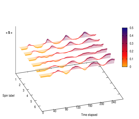
In order to describe spin transfer from spin-polarized incoming electrons to a spin chain, we show dynamics of the spins in the chain. We consider spins with initially pointing to the direction. For the parameters we choose, the electron wave packet no longer interacts with the chain at (in dimensionless units). Fig. 1 illustrates how the spins time-evolve while interacting with incoming electrons one after another. The site-independent electron-spin coupling is and the ferromagnetic coupling is , which is also site-independent, in units of the hopping parameter . The arrows depict as three-dimensional vectors for spatial as well as temporal behavior of individual spins, and is further visualized by colors. As discussed in Ref.kim05 , the coupling determines the degree of spin transfer, which depends on non-monotonically. Fig. 1 shows two distinct dynamical regimes. First, while an electron wave packet is striking the spin chain, the interaction term in causes spin transfer, and therefore spin flip. This will occur with every member of the spins with multiple reflections of the electron within the chain included. Once the electron has left the spin chain, however, the spins continue to evolve in time, but solely due to the term. The result is the oscillating behavior depending on the value of .
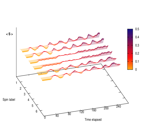
As mentioned earlier, parameterizing components of , one can envision a domain-structured spin chain. In Fig. 2, the coupling remains unchanged as in Fig. 1 while we choose a site-dependent for domains to form. The dynamics of spins is very different from the previous case. Because of the strong coupling between three spin pairs, two spins in each pair evolve simultaneously. The first and the last spin pairs oscillate against each other while the middle pair evolves almost monotonically. This overall behavior of three spin pairs is qualitatively the same as one of weakly coupled three local spins. Note that as more electrons are sent very little changes; for these parameters, five electrons are nearly sufficient to align the entire chain along the direction.
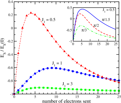
Another issue we wish to address in this paper concerns the excitations in the spin chain induced by the spin transfer process. We do not include a magnetic field in the Hamiltonian Eq. (3) because we investigate excitations only due to the relative spin configuration in the spin chain. If a magnetic field is included, additional excitations will be induced depending on the orientation of local spins with respect to the field. For investigation of the induced excitations, we consider only site-independent couplings and . The excitations induced by spin transfer are, in fact, associated with the energy transfer between the incident electrons and the spin chain. The energy of the chain is given by the expectation value of the Hamiltonian of the chain ; namely, . We demonstrate that depends on the coupling parameter , and energy is not monotonically transferred to the chain from incoming electrons. As local spins start to align with one another in the direction of the incident electron spin, energy would be transferred back to incoming electrons from the chain as illustrated in Fig. 3. This backwards energy transfer can be understood in a sense that excitation and de-excitation are relative in the absence of a magnetic field. Fig. 3 is for a spin chain interacting with incident electrons one by one. We set but choose various values of . The mean momentum of incident electrons is in the main frame while it varies in the inset to show that the energy transfer also depends on the momentum of the incident electrons. If is large enough, say , then no excitations occur and , where for a chain with local spins. Since there is no preferred direction due to the absence of a magnetic field, remains unchanged as all spins rotate in unison. This can be shown analytically.
In summary, we have outlined a quantum-mechanically rigorous framework with which one can calculate the spin transfer from a spin-polarized electron current to a spin chain. A brute force method is possible, but for a progression of incident electrons, this will quickly expand the Hilbert space to exceed the reach of modern computers. Application of the density matrix formalism not only solves this difficulty but also correctly deals with quantum entanglement inherent to the spin transfer problem. We have performed computations for a rather simplistic system; nonetheless, included are two essential elements of spin transfer; spins as quantum operators and entanglement.
As far as the physics of spin transfer is concerned, it is clear that the semi-classical assumption that the magnitude of the magnetization vector remains constant during spin transfer is generally violated. In particular, when the ferromagnetic exchange coupling is weak we find regimes where the magnitude of the spin vector can almost vanish. How this might alter our understanding of experimental observations will be the subject of further investigation.
This work was supported in part by the Natural Sciences and Engineering Research Council of Canada (NSERC), by ICORE (Alberta), and by the Canadian Institute for Advanced Research (CIAR). Numerical calculations have been performed using computational facilities of the Academic Information and Communication Technologies (AICT) and the WestGrid.
References
- (1) B.C. Choi, M. Belov, W.K. Hiebert, G.E. Ballentine, and M.R. Freeman, Phys. Rev. Lett. 86, 728 (2001).
- (2) M. Mansuripur, J. Appl. Phys. 63, 5809 (1988).
- (3) J.C. Slonczewski, J. Magn. Magn. Mater 159 L1, (1996); 195 L261, (1999).
- (4) L. Berger, Phys. Rev. B54, 9353, (1996); J. Appl. Phys. 89 5521 (2001).
- (5) E.B. Myers et al., Science 285, 867 (1999).
- (6) Y. Bazaliy, B.A. Jones, and S.-C. Zhang, Phys. Rev. B57, R3213 (1998).
- (7) X. Waintal, E.B. Myers, P.W. Brouwer, and D.C. Ralph, Phys. Rev. B62, 12317 (2000).
- (8) W. Kim and F. Marsiglio, Phys. Rev. B69, 212406 (2004).
- (9) W. Weber, S. Riesen, and H.C. Siegmann, Science 291, 1015 (2001).
- (10) S.A. Wolf et al., Science 294, 1488 (2001).
- (11) S.I. Kiselev et al., Nature 425, 380 (2003).
- (12) I.N. Krivorotov et al., Science 307, 228 (2005).
- (13) C.F. Hirjibehedin, C.P. Lutz, and A.J. Heinrich, Science 312, 1021 (2006).
- (14) M.A. Nielsen and I.L. Chuang, Quantum Computing and Quantum Information (Cambridge University Press, Cambridge, 2000).
- (15) M.N. Leuenberger and D. Loss, Nature 410, 789 (2001).
- (16) Y. Avishai and Y. Tokura, Phys. Rev. Lett. 87, 197203 (2001).
- (17) W. Kim, R.K. Teshima, and F. Marsiglio, Europhys. Lett. 69 595 (2005).
- (18) R.P. Feynman, Statistical Mechanics: A Set of Lectures, (Addison Wesley, Don Mills, 1972).
- (19) W. Kim, L. Covaci, and F. Marsiglio, Phys. Rev. B 74, 205120 (2006)
- (20) A.S. Nunez, R.A. Duine, P. Haney, and A.H. MacDonald, Phys. Rev. B 73, 214426 (2006).