Spectral densities of scale-free networks

Abstract

The spectral densities of the weighted Laplacian, random walk and weighted adjacency matrices associated with a random complex network are studied using the replica method. The link weights are parametrized by a weight exponent $\beta$. Explicit results are obtained for scale-free networks in the limit of large mean degree after the thermodynamic limit, for arbitrary degree exponent and $\beta$.

In a network representation of complex systems, their constituent elements and interactions between them are represented by nodes and links of a graph, respectively. Dynamical and structural properties of such systems can be understood first by studying linear problems defined on the network. A linear problem on a graph is associated with a matrix and the distribution of its eigenvalue spectrum is of interest. The real world networks are usually modeled as a random graph. The spectral density, also called the density of states, is the density of eigenvalues averaged over an appropriate ensemble of graph.

In this work, we study the spectral densities of several types of matrices associated with a scale-free network which has a power-law tail in the distribution of the number of incoming links to a node. The spectral densities in the thermodynamic limit are expressed in terms of solutions of corresponding non-linear functional equations and are solved analytically in the limit where the average incoming links per node is large. Implications of our results are discussed.

I Introduction

Many real world networks can be modeled as a scale-free network BarabasiA99 ; BoccalettiLMCH06 ; NewmanBW06 . In the scale-free network, the degree $d$, the number of incident links to a node, is distributed with a power-law tail decaying as $\sim d^{-\lambda}$ with the degree exponent $\lambda$ often in the range $2<\lambda<3$. Given such a network, one can consider several types of matrices associated with linear problems on the network. Many structural and dynamic properties of the network are then encoded in the eigenvalue spectra of such matrices and hence the distributions of their eigenvalue spectra are of interest. Since each of the real world networks may be viewed as a realization of certain random processes, the spectral density or the density of states is studied theoretically by averaging them over an appropriate ensemble.

One of such an ensemble is the static model GohKK01 ; LeeGKK04 which was motivated by its simulational simplicity. Being uncorrelated in links, it allows easier analytical treatments than other growing type models. Other closely related one is that of Chung and Lu ChungL02 . Recently in RodgersAKK05 , the replica method is applied to study the spectral density of the adjacency matrix of scale-free networks using the static model. The expression for the spectral density is derived in terms of a solution of a non-linear functional equation which were solved in the dense graph limit $p\rightarrow\infty$, $p$ being the mean degree. The explicit solution shows that the spectral density decays as a power law with the decay exponent $\sigma_{A}=2\lambda-1$ confirming previous approximate derivations DorogovtsevGMM03 and a rigorous result on the Chung-Lu model ChungLV03 .

In this paper, we extend RodgersAKK05 and study three other types of random matrices motivated from linear problems on networks. They are the weighted Laplacian $W$, the random walk matrix $R$ and the weighted adjacency matrix $B$, respectively. We set up the non-linear functional equations for each type of matrices and solve them in the dense graph limit $p\rightarrow\infty$. For the random walk matrix, we find its spectral density to follow the semi-circle law for all $\lambda$. For the weighted matrices, to be specific, the weights of a link between nodes $i$ and $j$ are given in the form of $(\langle d_{i}\rangle\langle d_{j}\rangle)^{-\beta/2}$ where $\langle d_{i}\rangle$ is the mean degree of node $i$ over the ensemble. This form of weights is motivated by recent works on complex networks BarratBPV04 ; MacdonaldAB05 ; MotterZK05 ; ZhouMK06 ; Korniss06 ; GucluKT07 ; OhLKK07 . When $\beta<1$, we find that the effect of $\beta$ on the spectral density is to renormalize $\lambda$ to $\tilde{\lambda}=(\lambda-\beta)/(1-\beta)$. The spectral density decays with a power law with exponents $\sigma_{W}=\tilde{\lambda}$ and $\sigma_{B}=(2\tilde{\lambda}-1)$, for $W$ and $B$, respectively for all $\tilde{\lambda}>2$. When $\beta=1$, the spectral density of $B$ reduces to the semi-circle law, the same as in $R$ while that of $W$ is bell-shaped. When $\beta>1$, we find that the spectral densities of $W$ and $B$ show a power-law type singular behavior near zero eigenvalue characterized by the spectral dimension $(\lambda-1)/(\beta-1)$.

This paper is organized as follows. In section 2, we generalize RodgersAKK05 in a form applicable to other types of matrices and present general expressions for the spectral density function in terms of the solution of non-linear functional equation. In sections 3, 4, and 5, we define and solve the weighted Laplacian, the random walk matrix and the weighted adjacency matrix, respectively, in the large $p$ limit. In section 6, we summarize and discuss our results.

II General Formalism

We consider an ensemble of simple graphs with $N$ nodes characterized by the adjacency matrix $A$ whose elements $A_{ij}=A_{ji}$ ($i\neq j$) are independently distributed with probability

$$P(A_{ij})=f_{ij}\delta(A_{ij}-1)+(1-f_{ij})\delta(A_{ij})$$ (1)

and $A_{ii}=0$. The degree of a node $i$ is $d_{i}=\sum_{j}A_{ij}$ and $\langle\dots\rangle$ below denotes an average over the ensemble.

In the static model of scale-free network GohKK01 , $f_{ij}$ is given as

$$f_{ij}=1-\exp(-pNP_{i}P_{j}),$$ (2)

where $P_{i}\propto i^{-1/(\lambda-1)}$ ($\lambda>2$) is the normalized weight of a node $i=1,\ldots,N$, related to the expected degree sequence as $\langle d_{i}\rangle=pNP_{i}$, and $p=\sum_{i}\langle d_{i}\rangle/N$ is the mean degree of the network. The degree distribution follows the power law $\sim d^{-\lambda}$. The Erdős-Rényi’s (ER’s) classical random graph ErdosR60 is recovered in the limit $\lambda\rightarrow\infty$, where $P_{i}=1/N$ which is called the ER limit below. In the model of Chung and Lu ChungL02 , $f_{ij}$ is taken as $f_{ij}=pNP_{i}P_{j}$ , with $P_{i}\propto(i+i_{0})^{-1/(\lambda-1)}$. When $2<\lambda<3$, $i_{0}$ should be $O(N^{(3-\lambda)/2})$ to satisfy $f_{ij}<1$ introducing an artificial cut-off in the maximum degree. In the following, we use the static model for ensemble averages but final results are the same for the two models in the thermodynamic limit $N\rightarrow\infty$.

Given a real symmetric matrix $Q$ of size $N$ associated with a graph, its spectral density, or the density of states, $\rho_{Q}(\mu)$ is obtained from the formula

$$\rho_{Q}(\mu)=\frac{2}{N\pi}{\rm Im}\frac{\partial\langle\log Z_{Q}(\mu)\rangle}{\partial\mu},$$ (3)

where

$$Z_{Q}(\mu)=\int_{-\infty}^{\infty}\left(\prod_{i}{\rm d}\phi_{i}\right)\exp\left(\frac{{\rm i}}{2}\mu\sum_{i}\phi_{i}^{2}-\frac{\rm i}{2}\sum_{ij}\phi_{i}Q_{ij}\phi_{j}\right)$$ (4)

with ${\rm Im}\mu\rightarrow 0^{+}$. For a class of matrices considered in this work, $Z_{Q}$ can be written in the form

$$Z_{Q}(\mu)=\int_{-\infty}^{\infty}\left(\prod_{i}{\rm d}\phi_{i}\right)\exp\left(\sum_{i}h_{i}(\phi_{i})+\sum_{i<j}A_{ij}V(\phi_{i},\phi_{j})\right).$$ (5)

Then following KimRKK05 and RodgersAKK05 we arrive at the expression

$$\rho_{Q}(\mu)=\frac{2}{n\pi}{\rm Im}\frac{\partial}{\partial\mu}\frac{1}{N}\sum_{i=1}^{N}\ln\int{\rm d}^{n}\phi\exp\left(\sum_{\alpha}h_{i}(\phi_{\alpha})+pNP_{i}\,g_{Q}\{\phi_{\alpha}\}\right),$$ (6)

where $\alpha$=$1,\ldots,n$ is the replica index, the limit $n\rightarrow 0$ is to be taken after, and $g_{Q}\{\phi_{\alpha}\}$ is a solution of the non-linear functional integral equation

$$g_{Q}\{\phi_{\alpha}\}=\sum_{i}P_{i}\frac{\int{\rm d}^{n}\psi\left(\exp(\sum_{\alpha}V(\phi_{\alpha},\psi_{\alpha}))-1\right)\exp\left(\sum_{\alpha}h_{i}(\psi_{\alpha})+pNP_{i}\,g_{Q}\{\psi_{\alpha}\}\right)}{\int{\rm d}^{n}\psi\exp\left(\sum_{\alpha}h_{i}(\psi_{\alpha})+pNP_{i}\,g_{Q}\{\psi_{\alpha}\}\right)}.$$ (7)

The derivation is valid when $S_{ij}=\exp(\sum_{\alpha}V(\phi_{i\alpha},\phi_{j\alpha}))-1$ satisfies the factorization property, that is, when $S_{ij}$ can be expanded into the form

$$S_{ij}=\sum_{J}a_{J}O_{J}(\phi_{i1},\ldots\phi_{in})O_{J}(\phi_{j1},\ldots\phi_{jn}),$$ (8)

where $J$ denotes a term of the expansion, $a_{J}$ and $O_{J}$ its coefficient and corresponding function, respectively. A crucial step in this derivation is the use of $\log(1+f_{ij}S_{ij})\approx pNP_{i}P_{j}S_{ij}$. This introduces a relative error of $\leq O(N^{2-\lambda}\log N)$ for $2<\lambda<3$ in both the static model and the Chung-Lu model and is neglected in the thermodynamic limit KimRKK05 ; Kim07 .

If $V(\phi,\psi)$ has the rotational invariance in the replica space, we may look for the solution of $g_{Q}\{\phi_{\alpha}\}$ in the form of $g_{Q}(x)$ with $x=\sqrt{\sum_{\alpha}\phi_{\alpha}^{2}}$. Then the angular integral can be evaluated and the $n\rightarrow 0$ limit can be taken explicitly. The sums over nodes are converted to integrals using

$$\frac{1}{N}\sum_{i}F(NP_{i})=(\lambda-1)\int_{0}^{1}u^{\lambda-2}F\left(\frac{(\lambda-2)}{(\lambda-1)}\frac{1}{u}\right){\rm d}u.$$ (9)

In the following sections, we apply this formalism to obtain formal expressions for the spectral densities of several types of matrices and evaluate them explicitly in the large $p$ limit. When $\mu$ is scaled to another variable $E$, we use the convention $\rho_{Q}(E)=\rho_{Q}(\mu)({\rm d}\mu/{\rm d}E)$ so that $\int\rho_{Q}(E){\rm d}E=1$.

III Weighted Laplacian

The weighted Laplacian $W$ considered in this section is defined as

$$W_{ij}=\frac{d_{i}\delta_{ij}-A_{ij}}{\sqrt{q_{i}q_{j}}}$$ (10)

where $A$ is the adjacency matrix and $d_{i}=\sum_{j}A_{ij}$ is the degree of node $i$, and $q_{i}$ are arbitrary positive constants. This is motivated by the linear problem of the type

$$\frac{{\rm d}\phi_{i}}{{\rm d}t}=-\frac{1}{q_{i}}\sum_{j}A_{ij}(\phi_{i}-\phi_{j})=-\sum_{j}\overline{W}_{ij}\phi_{j},$$ (11)

where $\overline{W}_{ij}=(d_{i}\delta_{ij}-A_{ij})/q_{i}$. For example, in the context of the synchronization, the input signal to a node from its neighbors may be scaled by a factor $d_{i}^{\beta}$ MotterZK05 ; OhLKK07 , which may be approximated as $\langle d_{i}\rangle^{\beta}$ LeeJS06 or to an average intensity of weighted networks ZhouMK06 . Also the problem has relevance to the Edward-Wilkinson process on network GucluKT07 . $\overline{W}$ and $W$ are similar to each other since $W=S^{1/2}\overline{W}S^{-1/2}$ with $S$ the diagonal matrix with elements $S_{ii}=q_{i}$. Eigenvalues of $W$ are positive real with minimum at the trivial eigenvalue 0.

When $q_{i}=1$ for all $i$, $W$ reduces to the standard Laplacian $L$ defined by

$$L_{ij}=d_{i}\delta_{ij}-A_{ij}.$$ (12)

In the literature, the Laplacian is sometimes defined by the normalized form

$$\overline{L}_{ij}=\left\{\begin{array}[]{ll}1&\mbox{if $i=j$ and $d_{i}\neq 0$},\\ -\frac{1}{\sqrt{d_{i}d_{j}}}&\mbox{if $A_{ij}=1$},\\ 0&\mbox{otherwise}.\end{array}\right.$$ (13)

We call $R\equiv I-\overline{L}$ the random walk matrix in this work and discuss it in the next section. We mention here that $W$ is a weighted version of the Laplacian of unweighted graphs while the Laplacian of weighted graphs would have been defined by $C_{ij}=(\sum_{k}A_{ik}/\sqrt{q_{i}q_{k}})\delta_{ij}-A_{ij}/\sqrt{q_{i}q_{j}}$ ZhouMK06 ; Korniss06 .

For $Q=W$ in (4), $Z_{W}(\mu)$ can be brought into the form (5) by a change of variable $\phi\rightarrow\sqrt{q_{i}}\phi$, with $h_{i}(\phi)=\frac{{\rm i}}{2}\mu q_{i}\phi^{2}$ and $V(\phi,\psi)=-\frac{{\rm i}}{2}(\phi-\psi)^{2}$. Inserting these into (6) and (7), and evaluating the angular integral, we obtain

$$\rho_{W}(\mu)=\frac{1}{\pi N}{\rm Re}\sum_{i}q_{i}\int_{0}^{\infty}y\exp(\frac{{\rm i}}{2}\mu q_{i}y^{2}+pNP_{i}\,g_{W}(y)){\rm d}y$$ (14)

with

$$g_{W}(x) = {\rm e}^{-{\rm i}x^{2}/2}-1$$ (15)

$$-x{\rm e}^{-{\rm i}x^{2}/2}\sum_{i}P_{i}\int_{0}^{\infty}J_{1}(xy)\exp(\frac{\rm i}{2}\mu q_{i}y^{2}-\frac{\rm i}{2}y^{2}+pNP_{i}\,g_{W}(y)){\rm d}y,$$

where $J_{1}(z)$ is the Bessel function of order one. In the ER limit ($NP_{i}=1$) and $q_{i}=1$, (14) and (15) reduce to equations (17) and (16) of BrayR88 , respectively.

The dense graph limit $p\rightarrow\infty$ is investigated by using the scaled function $G_{W}(x)=pg_{W}(x/\sqrt{p})$. Then in the limit $p\rightarrow\infty$, $G_{W}(x)=-\frac{\rm i}{2}x^{2}$ and

$$\rho_{W}(\mu)=\frac{1}{\pi N}{\rm Im}\sum_{i}\frac{q_{i}}{pNP_{i}-\mu q_{i}}$$ (16)

for arbitrary $q_{i}$. To be specific, we now set $q_{i}=\langle d_{i}\rangle^{\beta}=(pNP_{i})^{\beta}$ at this stage. $\beta$ is arbitrary and is called the weight exponent here. When the eigenvalue is scaled as

$$E=p^{\beta-1}(\lambda-2)^{\beta-1}(\lambda-1)^{1-\beta}\mu,$$ (17)

we find the spectral density in the dense graph limit as

$$\rho_{W}(E)=\frac{\lambda-1}{\pi}{\rm Im}\int_{0}^{1}\frac{u^{\lambda-\beta-1}}{1-u^{1-\beta}E}{\rm d}u.$$ (18)

This shows qualitatively different behaviors in the three regions of $\beta$.

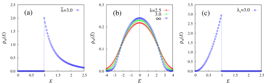
Figure 1: (Color online) The spectral density of the weighted Laplacian for weight exponent $\beta<1$ (a), $\beta=1$ (b), and $\beta>1$ (c). In (a) and (c), a typical curve is shown as a function of $E$ while in (b), the spectral density is shown as a function of $\overline{E}=\sqrt{p}(E-1)$ for several values of $\lambda$.

(i) $\beta<1$:

Eq. (18) is evaluated as

$$\rho_{W}(E)=\left\{\begin{array}[]{ll}0&\mbox{if $0<E<1$},\\ (\frac{\lambda-1}{1-\beta})E^{-(\lambda-\beta)/(1-\beta)}&\mbox{if $E>1$}.\end{array}\right.$$ (19)

Therefore, the spectra has a finite gap in $E$ and a power-law tail with an exponent $\sigma_{W}=(\lambda-\beta)/(1-\beta)$. The only effect of $\beta$ here is to renormalize $\lambda$ to

$$\tilde{\lambda}=\frac{\lambda-\beta}{1-\beta}.$$ (20)

Fig. 1(a) shows the graph of $\rho_{W}(E)$ for $\tilde{\lambda}=3$.

(ii) $\beta=1$:

The case $\beta=1$ needs a special treatment. When $\beta=1$, $E=\mu$ and $\rho_{W}(E)=\delta(E-1)$. However, if we expand the region near $E=1$ by introducing a new variable $\overline{E}$ by $\overline{E}=\sqrt{p}(E-1)$, we obtain non-trivial values for finite $\overline{E}$. The method and result are similar to that treated in BrayR88 for the ER case. Following BrayR88 , the function $g_{W}(x)$ in Eq. (15) is written in terms of $H(x)$, defined by

$$pg_{W}(p^{-1/4}x)=-{\rm i}\sqrt{p}x^{2}/2-x^{4}/8+H(x).$$ (21)

Then in the limit $p\rightarrow\infty$, (15) gives $H(x)={\rm i}\gamma(\overline{E})x^{2}/2$ and (14) gives $\rho_{W}(\overline{E})={\rm Im}\gamma(\overline{E})/\pi$, where $\gamma(\overline{E})$ is the solution of

$$\gamma=-\frac{(\lambda-1)}{\sqrt{2\pi}}\int_{-\infty}^{\infty}{\rm d}z{\rm e}^{-z^{2}/2}\int_{0}^{1}\frac{u^{\lambda-2}{\rm d}u}{\overline{E}+\gamma+z\sqrt{u(\lambda-1)/(\lambda-2)}}.$$ (22)

Fig. 1(b) shows the graph of $\rho_{W}(\overline{E})$ for several values of $\lambda$.

(iii) $\beta>1$:

In this case, (18) is evaluated as

$$\rho_{W}(E)=\left\{\begin{array}[]{ll}(\frac{\lambda-1}{\beta-1})E^{(\lambda-\beta)/(\beta-1)}&\mbox{if $0<E<1$}\\ 0&\mbox{if $E>1$}.\end{array}\right.$$ (23)

Thus $\rho_{W}(E)$ is non-zero for $0<E<1$ with a simple power. Such power-law dependence near the zero eigenvalue gives arise a long-time relaxation $\sim t^{-\lambda_{s}}$ with the spectral dimension RammalT83 ; AlexanderO82 ; BurdaCK01 ; DestriD02

$$\lambda_{s}=\frac{\lambda-1}{\beta-1}.$$ (24)

Fig.1(c) shows the graph of $\rho_{W}(E)$ for $\lambda_{s}=3$.

IV Random walk matrix

Consider a random walk problem defined as follows: When a random walker at a node $i$ sees $d_{i}$ neighbors, it jumps to one of them with equal probability. When a node $i$ is isolated so that $d_{i}=0$, the random walker is supposed not to move. Then the transition probability from node $i$ to $j$ is given by $\overline{R}_{ij}=A_{ij}/d_{i}$ if $d_{i}\neq 0$ and $\overline{R}_{ij}=\delta_{ij}$ if $d_{i}=0$. $\overline{R}$ can be brought into a symmetric form by a similarity transformation $R=T^{1/2}\overline{R}T^{-1/2}$, where $T$ is the diagonal matrix with elements $T_{ii}=1$ when $d_{i}=0$ and $T_{ii}=d_{i}$ when $d_{i}\neq 0$. The resulting symmetric matrix $R$, called the random walk matrix here, is

$$R_{ij}=\left\{\begin{array}[]{ll}1&\mbox{if $i=j$ and $d_{i}=0$},\\ \frac{1}{\sqrt{d_{i}d_{j}}}&\mbox{if $A_{ij}=1$},\\ 0&\mbox{otherwise.}\end{array}\right.$$ (25)

Being similar, $R$ and $\overline{R}$ have the same set of eigenvalues that are located within the range $|\mu|\leq 1$.

The isolated nodes integrate out of the partition function $Z_{R}(\mu)$ in (4), giving an additive term $n_{0}\delta(\mu-1)$ in the spectral density $\rho_{R}(\mu)$ where $n_{0}$ is the density of isolated nodes. For the remaining nodes, $R_{ij}=A_{ij}/\sqrt{d_{i}d_{j}}$ and, after a change of variable $\phi_{i}\rightarrow\sqrt{d_{i}}\phi_{i}$, $Z_{R}(\mu)$ can be brought into the form (5) with $V(\phi,\psi)=\frac{\rm i}{2}\mu(\phi^{2}+\psi^{2})-{\rm i}\phi\psi$ and $h_{i}(\phi)=-\epsilon\phi^{2}$ with $\epsilon\rightarrow 0^{+}$ to ensure convergences. Since $A_{ij}=0$ anyway for isolated nodes, the sums in (5) is extended to all nodes. Plugging this into (6) and (7), we find

$$\rho_{R}(\mu)=n_{0}\delta(\mu-1)+\frac{p}{\pi}{\rm Re}\sum_{i}P_{i}\int_{0}^{\infty}yg_{R}(y)\exp(pNP_{i}[g_{R}(y)-1]){\rm d}y$$ (26)

with

$$g_{R}(x)={\rm e}^{{\rm i}\mu x^{2}/2}-x\sum_{i}P_{i}\int_{0}^{\infty}J_{1}(xy)\exp(\frac{\rm i}{2}\mu(x^{2}+y^{2})+pNP_{i}[g_{R}(y)-1]){\rm d}y.$$ (27)

When $p\rightarrow\infty$, all nodes belong to the percolating giant cluster LeeGKK04 and $n_{0}$ vanishes. To obtain the spectral density in the limit $p\rightarrow\infty$, we scale $\mu=p^{-1/2}E$ and $g_{R}(x)=1+G_{R}(p^{1/4}x)/p$. Then from (27), $G_{R}(x)$ is determined as $G_{R}(x)=-ax^{2}/2$ with $a$ being a solution of $a^{2}+{\rm i}Ea-1=0$ and from (26), $\rho_{R}(E)={\rm Re}(\pi a)^{-1}$. This gives the semi-circle law for all $\lambda$:

$$\rho_{R}(E)=\frac{1}{\pi}\sqrt{1-\frac{E^{2}}{4}}$$ (28)

for $|E|\leq 2$ and 0 otherwise.

V Weighted adjacency matrix

In this section, we consider the weighted version of $A$ defined by

$$B_{ij}=\frac{A_{ij}}{\sqrt{q_{i}q_{j}}},$$ (29)

where $q_{i}$ are arbitrary positive constants. This is motivated by the weighted networks whose link weights are product of quantities associated with the two nodes at each end of the linkBarratBPV04 ; MacdonaldAB05 . Later on for explicit evaluations, we take $q_{i}$ to be $q_{i}=\langle d_{i}\rangle^{\beta}=(pNP_{i})^{\beta}$ with arbitrary $\beta$. When $\beta=0$, we recover $A$ treated in RodgersAKK05 while when $\beta=1$, $B_{ij}=A_{ij}/\sqrt{\langle d_{i}\rangle\langle d_{j}\rangle}$ may be considered as an approximation to $R$ and is treated in ChungLV03 . With a change of variable $\phi_{i}\rightarrow\sqrt{q_{i}}\phi_{i}$ in (4), $Z_{B}$ is of the form (5) with $h_{i}(\phi)=\frac{\rm i}{2}\mu q_{i}\phi^{2}$ and $V(\phi,\psi)=-{\rm i}\phi\psi$. Then we find

$$\rho_{B}(\mu)=\frac{1}{\pi N}{\rm Re}\sum_{i}q_{i}\int_{0}^{\infty}y\exp(\frac{\rm i}{2}\mu q_{i}y^{2}+pNP_{i}\,g_{B}(y)){\rm d}y$$ (30)

with

$$g_{B}(x)=-\sum_{i}P_{i}\int_{0}^{\infty}xJ_{1}(xy)\exp(\frac{\rm i}{2}\mu q_{i}y^{2}+pNP_{i}g_{B}(y)){\rm d}y$$ (31)

for arbitrary $q_{i}$.

Specializing to the case where $q_{i}=\langle d_{i}\rangle^{\beta}=(pNP_{i})^{\beta}$, the limit $p\rightarrow\infty$ is investigated by scaling $\mu$ to $E$ by

$$E=p^{\beta-\frac{1}{2}}(\lambda-2)^{\beta-1}(\lambda-1)^{1-\beta}\mu,$$ (32)

and $g_{B}(x)=G_{B}(p^{1/4}x)/p$. Then $G_{B}(x)=-\frac{\rm i}{2}Eb(E)x^{2}$ and

$$\rho_{B}(E)=-\frac{E}{\pi}{\rm Im}b^{2}(E)$$ (33)

with $b(E)$ as the solution of

$$E^{2}b=(\lambda-1)\int_{0}^{1}\frac{u^{\lambda-2}}{u^{1-\beta}-b}{\rm d}u.$$ (34)

In the ER limit, we recover the semi-circle law regardless of $\beta$. For finite $\lambda$, we consider three regions of $\beta$ separately.

(i) $\beta<1$:

A change of integration variable in (34) leads to

$$\ {}_{2}F_{1}\left(1,\frac{\lambda-1}{1-\beta};\frac{\lambda-\beta}{1-\beta};\frac{1}{b}\right)=-b^{2}E^{2}$$ (35)

where $\ {}_{2}F_{1}(1,c-1;c;z)=(c-1)\int_{0}^{1}t^{c-2}/(1-tz){\rm d}z$ is the hypergeometric function. Eq. (35) is a generalization of RodgersAKK05 which is a special case of $\beta=0$. One notes that the effect of $\beta$ is again to renormalize $\lambda$ to $\tilde{\lambda}=(\lambda-\beta)/(1-\beta)$ and the results of RodgersAKK05 applies here when its degree exponent is replaced by the effective one. In particular, the spectral density is symmetric in $E$, has the power-law tail $\sim|E|^{-\sigma_{B}}$ with an exponent

$$\sigma_{B}=2\tilde{\lambda}-1=\frac{2\lambda-\beta-1}{1-\beta}$$ (36)

and an analytic maximum $(\tilde{\lambda}-1)/(\tilde{\lambda}\pi)$ at $E=0$. Fig. 2(a) shows the graph of $\rho_{B}(E)$ for several values of $\tilde{\lambda}$.

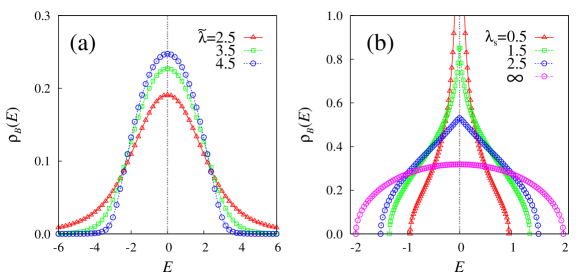
Figure 2: (Color online) The spectral density of the weighted adjacency matrix with weight exponent $\beta<1$ in (a) and $\beta>1$ in (b), for several values of effective degree exponents $\tilde{\lambda}$ (a) and $\lambda_{s}$ (b), respectively.

(ii) $\beta=1$:

In this case, $b$ in (34) is simply determined from $E^{2}b=1/(1-b)$ and the spectral density becomes the semi-circle law:

$$\rho_{B}(E)=\frac{1}{\pi}\sqrt{1-\frac{E^{2}}{4}}$$ (37)

for $|E|\leq 2$ and 0 for $|E|>2$ for all $\lambda$. The same is proved in  ChungLV03 for sufficiently large but finite $p$ while we have taken the limit $p\rightarrow\infty$. $B$ at $\beta=1$ being an approximation of $R$, it is not surprising to see the same results for the two cases.

(iii) $\beta>1$:

In this case, it is convenient to bring (34) into the form

$$E^{2}=\left(\frac{\lambda_{s}}{\lambda_{s}+1}\right)\frac{1}{b}\ _{2}F_{1}(1,\lambda_{s}+1;\lambda_{s}+2;b).$$ (38)

with $\lambda_{s}=(\lambda-1)/(\beta-1)$. The right hand-side of (38) as a function of real $b$ takes a minimum value $E_{c}^{2}$ at $0<b_{c}<1$ and increases to infinity as $b\rightarrow 0^{+}$ or $b\rightarrow 1^{-}$. Thus for $|E|>E_{c}$, $b(E)$ is real and $\rho_{B}(E)=0$. As $|E|$ decreases from $E_{c}$, $\rho_{B}(E)$ rises with a square root singularity since the righthand side of (38) is analytic at $b_{c}$. It is interesting to note that the behavior of $\rho_{B}(E)$ at $E=0$ is non-analytic. When $0<\lambda_{s}<1$, it diverges as

$$\rho_{B}(E)\sim\frac{\lambda_{s}}{2\cos(\frac{\pi}{2}\lambda_{s})}|E|^{-(1-\lambda_{s})}$$ (39)

while, for $\lambda_{s}>1$, its singular part is masked by the analytic part and it takes the finite maximum value

$$\rho_{B}(0)=\frac{1}{\pi}\frac{\lambda_{s}}{\lambda_{s}-1}.$$ (40)

At $\lambda_{s}=1$, it diverges logarithmically:

$$\rho_{B}(E)\sim\frac{1}{\pi}\log\frac{1}{|E|}.$$ (41)

Fig. 2(b) shows the graph of $\rho_{B}(E)$ for several values of $\lambda_{s}$.

VI Summary and Discussion

In this work, we derived the spectral densities of three types of random matrices, the weighted Laplacian $W$, the random walk matrix $R$, and the weighted adjacency matrix $B$, of the static model in the dense graph limit after the thermodynamic limit. Our results apply to the model of Chung-Lu also. In fact, they apply to other models as long as $f_{ij}$ in (1) is a function of $pNP_{i}P_{j}$ and satisfy $f_{ij}\leq pNP_{i}P_{j}$.

With weights of the form $q_{i}=\langle d_{i}\rangle^{\beta}$, they show varying behaviors depending on the degree exponent $\lambda$ and the weight exponent $\beta$. The spectrum follows the semi-circle law for $R$, and at the $\beta=1$ point of $B$ for all $\lambda$. The $\beta=1$ point of $W$ is closely related to $I-B$ or $I-R$, but its spectral density is not of the semi-circle law but is bell-shaped. When $\beta<1$, the degree exponent is renormalized to $\tilde{\lambda}$ given in (20) and the spectral density shows a power law decay with exponent $\sigma_{W}=\tilde{\lambda}$ and $\sigma_{B}=2\tilde{\lambda}-1$ for $W$ and $B$, respectively. When the eigenvalue spectrum has a long tail decaying as $\sim\mu^{-\sigma}$, the maximum eigenvalue of a finite system is expected to scale with $N$ as $\mu_{\rm N}\sim N^{1/(\sigma-1)}$ while the natural cutoff of degree in the scale-free network is $d_{\rm max}\sim N^{1/(\lambda-1)}$. The maximum eigenvalue of the weighted Laplacian $W$ may be taken as $W_{11}\sim d_{\rm max}^{1-\beta}$ for $\beta<1$ in the first order perturbation approximation. This simple argument explains the power of the tail $\sigma_{W}=\tilde{\lambda}=(\lambda-\beta)/(1-\beta)$ for $W$. A similar argument applied to $(B^{2})_{11}\sim d_{\rm max}^{1-\beta}$ gives the decay exponent $\sigma_{B}=2\tilde{\lambda}-1$ for $B$.

When $\beta>1$, the spectral densities of $W$ and $B$ are non-zero within a finite interval of the scaled eigenvalue $E$ and are associated with the spectral dimension $\lambda_{s}$ given in (24). For $W$, it is a simply power $\sim E^{\lambda_{s}-1}$ in $0<E<1$, while for $B$, it is symmetric in $E$ and singular at $|E|=0$ with exponent $\lambda_{s}-1$. They both diverge as $E\rightarrow 0$ when $0<\lambda_{s}<1$.

When $p$ is finite, the spectra is very complicated and is not well understood. For small $p$ at least, one expects infinite number of delta peaks on the spectrum BauerG01 . In the dense graph limit $p\rightarrow\infty$, those delta peaks have disappeared. Even though our explicit results are for the limit $p\rightarrow\infty$, the limit is taken after the thermodynamics limit $N\rightarrow\infty$, and physically they would be a good approximation for $1\ll p\ll N$ in finite systems. In the synchronization problem on networks, the eigenratio $R=\mu_{N}/\mu_{2}$ of $W$ is of interest BarahonaP02 . From (19), one may estimate $\mu_{N}\sim N^{{(1-\beta)}/{(\lambda-1)}}$ and $\ln R\sim\frac{1-\beta}{\lambda-1}\ln N$ for $\beta<1$, assuming that $N$-dependence of $\mu_{2}$ is slower than the power law. Similarly, from (23), one gets $\ln R\sim\frac{\beta-1}{\lambda-1}\ln N$ for $\beta>1$. Such $\beta$-dependence of $R$ is corroborated with numerical results for a similar matrix studied in MotterZK05 .

The spectral properties of Laplacian on weighted networks, $C_{ij}=(\sum_{k}B_{ik})\delta_{ij}-B_{ij}$ or its normalized version $D_{ij}=\delta_{ij}-B_{ij}/\sqrt{\sum_{k}B_{ik}\sum_{k}B_{jk}}$ are also of interestZhouMK06 ; Korniss06 . Unfortunately, the formalism leading to (6) and (7) cannot be applied to these cases since the factorization property (8) is not satisfied.

References

(1) A.-L. Barabási and R. Albert, Science 286, 509 (1999).
(2) S. Boccaletti, V. Latora, Y. Moreno, M. Chavez,
and D.-U. Hwang, Phys. Rep. 424, 175 (2006).
(3) M. E. J. Newman, A.-L. Barabási, and D. J. Watts,
“The structure and dynamics of networks” (Princeton
University Press, Princeton, 2006).
(4) K.-I. Goh, B. Kahng and D. Kim, Phys. Rev. Lett. 87, 278701 (2001).
(5) D.-S. Lee, K.-I. Goh, B. Kahng and D. Kim,
Nucl. Phys. B 696, 351 (2004).
(6) F. Chung and L. Lu, Ann. Comb. 6, 125
(2002).
(7) G. J. Rodgers, K. Austin, B. Kahng and D. Kim,
J. Phys. A:Math. Gen. 38, 9431 (2005).
(8)S. N. Dorogovtsev, A. V. Goltsev, J. F. F. Mendes,
and A. N. Samukin, Phys. Rev. E 64, 046109 (2003).
(9) F. Chung, L. Lu and V. Vu, Proc. Nat. Acad. Sci. U.S.A. 100, 6313 (2003).
(10) A. Barrat, M. Barthelemy, R. Pastor-Satorras, and A.
Vespignani, Proc. Nat. Acad. Sci. U.S.A. 101, 3747 (2004).
(11) P. J. Macdonald, E. Almaas and A.-L. Barabási, Europhys. Lett.
72, 308 (2005).
(12) A.E. Motter, C. Zhou and J. Kurths, Europhys.
Lett. 69, 334 (2005).
(13) C. Zhou, A.E. Motter and J. Kurths,
Phys. Rev. Lett. 96, 034101 (2006).
(14) G. Korniss, arXiv:cond-mat/0609098.
(15) H. Guclu, G. Korniss, and Z. Toroczkai,
arXiv:cond-mat/0701301.
(16) E. Oh, D.-S. Lee, B. Kahng, and D. Kim, Phys. Rev. E 75, 011104 (2007).
(17) P. Erdős and A. Rényi, Publ. Math. Inst. Hung. Acad. Sci. Ser. A
5, 17 (1960).
(18) D.-H. Kim, G. J. Rodgers, B. Kahng and D. Kim,
Phys. Rev. E 71, 056115 (2005).
(19) D. Kim, (unpublished).
(20) J.-S. Lee, K.-I. Goh, B. Kahng and D. Kim, Eur.
Phys. J. B 49, 231 (2006).
(21) A. J. Bray, and G. J. Rodgers, Phys. Rev. B 38, 11461 (1988).
(22) R. Rammal and G. Toulouse, J. Physique Lett.
44, L13 (1983).
(23) S. Alexander and R. Orbach, J. Physique
Lett. 43, L625 (1982).
(24) Z. Burda, J. D. Correia and A. Krzywicki, Phys.
Rev. E 64, 046118 (2001).
(25) C. Destri and L. Donetti, J. Phys. A: Math. Gen.
35, 9499 (2002).
(26) M. Bauer and O. Golinelli, J. Stat. Phys. 103, 301 (2001).
(27) M. Barahona and L. M. Pecora, Phys. Rev. Lett.
81, 054101 (2002).