Localization of particles in harmonic confinement: Effect of the interparticle interaction

Abstract

We study the localization of particles rotating in a two-dimensional harmonic potential by solving their rotational spectrum using many-particle quantum mechanics and comparing the result to that obtained with quantizing the rigid rotation and vibrational modes of localized particles. We show that for a small number of particles the localization is similar for bosons and fermions. Moreover, independent of the range of the interaction the quantum mechanical spectrum at large angular momenta can be understood by vibrational modes of localized particles.

I introduction

Interacting particles rotating in a harmonic confinement has become an experimentally realizable quantum system which has attracted plenty of attention during the last decade. The experiments in semiconductor quantum dots in the presence of a magnetic field showed Hund’s ruletarucha1996 and properties related to the quantum Hall liquidsmceuen1991 ; oosterkamp1999 . In increasing magnetic field the electrons, polarized by the field, first form so-called maximum density dropletmacdonald1993 , which is the finite electron number counterpart of the integer quantum Hall effect, and then are expected to form fractional quantum Hall liquidlaughlin1983 ; maksym1990 ; wojs1997 and eventually get localized to a Wigner crystalmaksym1996 .

The weakly interacting boson and fermion gases in atomic traps are other systems where particles move in a nearly harmonic trap. The traps can be three-dimensional or quasi-two-dimensional. Rotating laser field has been used to put the atom cloud in rotational motion which has lead to observation of vortices in both boson and fermion systemsmadison2000 ; abo2001 ; zwierlein2005 .

The experiments have inspired numerous theoretical studies on the properties of rotational quantum states of particles in a harmonic confinement. For quantum dots these studies have revealed several kinds of internal symmetry breakings of the system: Spin-density waveskoskinen1997 , broken symmetry edgereimann1999 , vortex formationsaarikoski2004 ; manninen2005 and electron localizationmuller1996 ; yannouleas1999 ; reimann2000 . In the case of boson and fermion condensates the theoretical research has concentrated on quite small angular momenta and has mainly been interested in vortex formationbutts1999 ; mottelson1999 ; bertsch1999 ; toreblad2004 ; reimann2006a , although localization by rotation has also been studiedmanninen2001 ; romanovsky2006 ; reimann2006 . It has been observed that both the vortex formationtoreblad2004 and the localizationreimann2006 are qualitatively similar for both types of particles, and that the type of the interparticle interaction does not seem to play an important role.

In this paper we will study in detail the limit of the particle localization to a ’Wigner molecule’ where the many-particle spectrum can be determined by combining classical vibrational modes to the rigid rotation of the ’molecule’. In the case of electrons this limit was studied in detail by Maksymmaksym1996 ; maksym2000 and later by usnikkarila2007 . Here we will extend this work to bosonic systems and also study the effect of the range of the interparticle interaction.

The paper is organized as follows. In Section II we introduce the models and discuss an exactly solvable model of harmonic interparticle interaction. In Section III we present results, first for seven particles interacting with Coulomb interaction and then study the effect of the range of the interaction using as an example four particles interacting with a Gaussian interaction. The conclusions are given in Section IV.

II Theoretical models

II.1 Quantum mechanics in the lowest Landau level

We assume a generic model of spinless fermions or bosons in a two-dimensional harmonic potential. The Hamiltonian is on the form

$$H=-\frac{\hbar^{2}}{2m}\sum_{i}^{N}\nabla_{i}^{2}+\sum_{i}^{N}\frac{1}{2}m\omega_{0}^{2}r_{i}^{2}+\sum_{i<j}^{N}v(|{\bf r}_{i}-{\bf r}_{j}|),$$ (1)

where $N$ is the number of particles and $m$ the electron mass and $\omega_{0}$ the oscillation frequency of the confining potential. The variable ${\bf r}=(x,y)$ is a two-dimensional position vector. The interparticle potential $v$ is either the Coulomb interaction or a Gaussian repulsion:

$$v(r)=\frac{e^{2}}{4\pi\epsilon_{0}r}\quad{\rm or}\quad v(r)=\frac{1}{\pi\sigma^{2}}e^{-r^{2}/\sigma^{2}}.$$ (2)

We solve the many-particle problem for a fixed angular momentum using the single particle basis of the lowest Landau level (LLL):

$$\psi_{\ell}(r,\phi)=A_{\ell}r^{\ell}e^{-m\omega_{0}r^{2}/2\hbar}e^{i\ell\phi},$$

where $\ell$ is the single-particle angular momentum and $A_{\ell}$ a normalization factor. The restriction to the LLL is a good approximation when total angular momentum $L$ is relatively large, $L\gtrsim N(N-1)$ manninen2001 ; jain2005a , corresponding to the filling factor of about $\nu\lesssim 1/2$ of the LLL. At this point it is convenient to stress that, when we consider electrons, we do not explicitly include magnetic field in our calculations. Assuming complete polarization, the only effect of the magnetic field has, is to increase the total angular momentum.

We present our results in terms of the total angular momentum, which can be related to the filling fraction of the LLL by $\nu\approx N(N-1)/2L$. Angular momenta $L=qN(N-1)/2$ then correspond to the fractional quantum Hall liquid with $\nu=1/q$, where $q$ is the exponent of the Laughlin wave functionlaughlin1983 (Eq. (4) below).

The restriction of the basis to the LLL gives some important exact results about the properties of the quantum states. These can be seen by writing the Hamiltonian (1) in the occupation number formalism as

$$\hat{H}=\hat{H}_{0}+\lambda\hat{V}=\hbar\omega_{0}N+\sum_{\ell}\hbar\omega_{0}\ell c_{\ell}^{\dagger}c_{\ell}+\lambda\sum_{ijkl}v_{ijkl}c_{i}^{\dagger}c_{j}^{\dagger}c_{l}c_{k},$$ (3)

where $c_{\ell}^{\dagger}$ creates a particle in the LLL. The states are written as $|n_{0}n_{1}n_{2}\cdots\rangle$ where the subsrcipt refers to the single particle angular momentum $\ell$.

We notice immediately that for a fixed total angular momentum $L=\sum_{\ell}n_{\ell}$ the diagonal term $\hat{H}_{0}$ of the Hamiltonian gives a constant $\hbar\omega_{0}(L+N)$, i.e. it is independent of the configuration. The diagonalization of the Hamiltonian thus equals to diagonalization of the interaction part $\hat{V}$ of the Hamiltonian, which gives directly the interaction energy $\Delta E=\langle\Psi|\hat{V}|\Psi\rangle$. Moreover, this means that the structure of the quantum states are independent of $\omega_{0}$ and the coupling constant $\lambda$, which have only the roles of giving the distance and energy scales.

In the case of bosons the state with $L=0$ is the Bose condensate where $n_{0}=N$ and all the other states are empty. for example, for seven bosons the state is $|7000\cdots\rangle$. In the case of fermions the lowest possible angular momentum is $L_{\rm MDD}=N(N-1)/2$ and the state is the so-called maximum density dropletmacdonald1993 $n_{i}=1$ for $i<N$ and this state for seven fermions is $|111111100\cdots\rangle$. The only possible state at for seven bosons at $L=1$ is $|61000\cdots\rangle$ and the corresponding state for seven fermions at $L=L_{\rm MDD}+1$ is $|11111101000\cdots\rangle$.

It follows that the interaction energy of the $L=0$ (or MDD) state equals to that of the $L=1$ (or $L_{\rm MDD}+1$) state, for any two-body interaction. This is due to the fact that the $L=1$ state is the center of mass excitation of the $L=0$ state. In the LLL the two lowest angular momentum states for both bosons and fermions are thus completely fixed by the basis and, consequently, are independent of the interparticle interaction.

In the case of the delta function interaction, the spinless fermions do not feel the interaction due to the Pauli exclusion principle. The MDD can be written in the form of the Laughlin wave function (without normalization) as

$$\Psi_{q}=\prod_{i<j}^{N}(z_{i}-z_{j})^{q}e^{\sum m\omega_{0}^{2}|z_{k}|^{2}/2\hbar},$$ (4)

where $z=x+iy$, and the exponent $q=1$ corresponding to the filling factor $\nu=1/q=1$. Since any wave function for higher angular momenta can be written as a symmetric polynomial times the above, the effect of the delta function interaction disappears. In the case of bosons the delta function interaction has an effect up to the angular momentum $L=N(N-1)$ when a symmetric wave function of the type of Eq. (4) can be reached, with $q=2$.

It turns out that also for long range interactions, even for the Coulomb interaction, the Laughlin type wave function becomes rather accurate for $q=3$ and 5 for fermions and for $q=2$ and 4 for bosons, while at even higher values of angular momenta the particles localize to Wigner molecules which rigidly rotate in the harmonic well.

While the Laughlin state gives good estimates for the wave function only for particular angular momenta, the composite fermion picture of Jainjain1989 ; jain1990 ; jeon2004 gives estimates for all angular momenta. It is important to note that both Laughlin and Jain wave functions are derived from very general arguments and are completely independent of the interparticle interactions.

The repulsive harmonic interaction

$$v(|{\bf r}_{i}-{\bf r}_{j}|)=-\lambda|{\bf r}_{i}-{\bf r}_{j}|^{2}$$ (5)

is exactly solvablelawson1980 ; johnson1992 ; ruuska2005 . The resulting interaction energy of the lowest state as a function of the angular momentum is for bosons ruuska2005

$$\Delta E(L)=-\frac{\lambda}{\omega_{0}}N(N-1)-\frac{\lambda}{\omega_{0}}NL\theta(L-2)$$ (6)

where $\theta$ is the step function. Due to the symmetry of the interaction the degeneracy of each state is large. Note that the interaction energy in this model decreases linearly with $L$.

II.2 Classical particles

Classical electrons in a 2D harmonic potential arrange in consecutive circles i.e. they form Wigner moleculesbolton1993 ; bedanov1994 . The molecule can have angular momentum due to the center of mass rotation or due to the rigid rotation of the molecule. In addition the molecule can have internal vibrational motion. The internal vibrational modes can then be found by solving the dynamical matrix. We are interested in the excitations of a rotating system and therefore we have to solve the internal vibrations in a rotating frame of reference. For quantum dots this was first done by Maksymmaksym1995 ; maksym1996 who used the Eckart rotating frame. We use a more straigthforward method where the Newton equations of motion are determined in a standard rotating frame, taking into account the Coriolis forcegoldstein1969 . We fix the rotation frequency $\omega_{r}$ which determines the total angular momentum $L$ of the rotating molecule.

The equilibrium positions of the particles depend naturally on the angular frequency and total angular momentum $L=I\omega_{r}$, where $I$ is the moment of inertia $I=m\sum r_{i}^{2}$. The classical energy

$$E_{\rm cl}^{0}(L)=\frac{1}{2}m\omega_{0}\sum_{i}^{N}r_{i}^{2}+\sum_{i<j}v({\bf r}_{i}-{\bf r}_{j})+\frac{L^{2}}{2I}$$ (7)

is minimized in order to solve the equilibrium configuration. The interparticle interaction $v(|{\bf r}_{i}-{\bf r}_{j}|)$ can be either Coulombic or Gaussian just like when solving the energy spectra of corresponding quantum mechanical systems.

In this article we report results for up to seven bosons and fermions. The eigenfrequencies can be solved analytically (or numerically) from the equations of motion in the rotating frame: The Newton equations are linearized around around the equilibrium positions of the particles and the vibrational modes are obtained with matrix algebra. When the classical vibrational frequencies are solved we quantize the energies with canonical quantizationashcroft1976 and get an estimate for the total quantum mechanical energy, which in general can be written as

$$E_{\rm cl}(L)=E_{\rm cl}^{0}(L)+\sum_{k}\hbar\omega_{k}(L)(n_{k}+\frac{1}{2})+\hbar\omega_{0}(n_{\rm CM}+1),$$ (8)

where $\omega_{k}(L)$ is the vibrational frequency determined in the rotating frame with angular momentum $L$, $n_{k}=0,~{}1,~{}2,\cdots$, and the last term corresponds to the center of mass excitations. The symmetry or antisymmetry requirement of the total quantum state dictates which vibrational states are allowed for a given $L$. For this reason we have to determine the symmetry properties of the vibrational modes and use group theorytinkham1964 ; ruan1995 ; maksym1996 ; koskinen2001 ; koskinen2002 to resolve the allowed states. Using the notations of Maksymmaksym1996 we have the following requirements for fermions

$$L+\sum_{i}n_{i}k_{i}=\bigg{\{}\begin{array}[]{ll}0\text{ mod }m&\text{ for }m=\text{odd}\\ m/2\text{ mod }m&\text{ for }m=\text{even}.\end{array}$$

The corresponding requirement for both even and odd number of bosons is

$$L+\sum_{i}n_{i}k_{i}=0\text{ mod }m.$$

The symbols $n_{i}$ refer to the number of excitations of mode $\omega_{i}$ and the number $k_{i}$ to the symmetry property of the same mode (rotation by $2\pi k/m$ is presented by $\exp(i2\pi k/m)$)maksym1996 .

The classical system with a repulsive harmonic interaction can also be solved analytically. For the lowest energy state as a function of the angular momentum we get

$$E(L)=L\sqrt{\omega_{0}^{2}-2N\lambda}.$$ (9)

Quantizing this and taking into account the zero point energy, the interaction energy will be

$$\begin{split}\Delta E(L)=&N\omega_{0}\sqrt{1-\frac{2(N-1)\lambda}{\omega_{0}^{2}}}\\ &+L\omega_{0}\sqrt{1-\frac{2N\lambda}{\omega_{0}^{2}}}-(N+L)\omega_{0},\end{split}$$ (10)

which for small $\lambda$ gives the result of Eq. (6). Notice that for $\omega_{0}^{2}<2N\lambda$ the harmonic potential is not strong enough for confining the particles.

We should also notice that in the case of the delta function interaction the classical system does not have any vibrational modes, but the particles behave like noninteracting particles (the collision probability is zero).

III Results

III.1 Seven particles with Coulomb interaction

We have considered four and seven bosons and fermions with different interparticle interactions. We remind the reader that in the LLL the results are independent of $\omega_{0}$, apart from the energy scale. It is then convenient to present the results in atomic units ($m=\hbar=e=a_{0}=1$). We use $\omega_{0}=1$ for the Gaussian interaction and $\omega_{0}=1/2$ for the Coulomb interaction.

The classical model has been studied for electrons in quantum dots by Maksym et almaksym1996 ; maksym2000 , Matulis and Anisimovasmatulis2005 and by usnikkarila2007 . We will first demonstrate that the same model works also for bosons interacting with the Coulomb interaction. Since the earlier computations have been restricted to six or less electrons we do this comparison for seven particles.

The classical problem of seven charged particles in a 2D harmonic potential can be solved analytically by first determining the classical minimum energy (7) at the equilibrium in the rotating frame and then solving the dynamical matrix. The lowest energy classical configuration is a hexagon of six particles surrounding the seventh particle at the origin. This geometry naturally has a six-fold rotation axis. The other stable classical geometry is a seven-fold ring. However, its energy is so much higher that it does not contribute to the low-energy rotation-vibration spectrum.

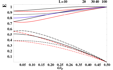
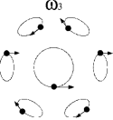
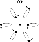
Figure 1: Upper panel: Classical vibrational frequencies as a function of the angular velocity of the rotating Wigner molecule with seven charged particles. The breathing mode is shown as a dotted line. The dashed and solid lines show other modes for seven electrons (in atomic units with $\omega_{0}=0.5$). Lower panel: Modes of the low energy vibrations (see text). Mode $\omega_{5}$ is similar to the mode $\omega_{3}$ (and degenerate at $\omega_{r}=0$) but the motion of the particles is opposite to that of mode $\omega_{3}$. In mode $\omega_{4}$ the particle at the center does not move. Mode $\omega_{7}$ is similar to mode $\omega_{4}$ (degenerate at $\omega_{r}=0$) but the particles move opposite direction. Note that in mode $\omega_{6}$ the orbits of the particles are the same as in modes $\omega_{4}$ and $\omega_{7}$ but the particles are at different phases.

The classical vibrational frequencies (except the center of mass mode) for 7 particles are shown in Fig. 1. The eigenfrequencies are shown as a function of the angular velocity of the rotation $\omega_{r}$. The angular momentum of the system increases rapidly and diverges as $\omega_{r}\rightarrow\omega_{0}$ (0.5 in this case). Some values of the angular momenta are shown in the figure. We notice that all frequencies approach to either $0$ or $2\omega_{0}$. One of the internal vibration energy is on the form $\omega_{\rm bm}=\sqrt{3\omega_{0}^{2}+\omega_{r}^{2}}$, and it is shown in the figure as a dotted line. This is a well known result for electrons forming one single ringschweigert1995 ; maksym1996 and it is called the breathing mode. The most interesting modes are the ones that approach $0$. We have labeled these low-energy modes as $\omega_{3}$ (lowest mode, plotted as red dashed line, $\omega_{3}\approx 0.4$ when $\omega_{r}=0$), $\omega_{5}$ (dashed line, is degenerate with $\omega_{3}$ when $\omega_{r}=0$), $\omega_{6}$ (solid line), $\omega_{4}$ (red dashed line, $\omega_{4}\approx 0.55$ when $\omega_{r}=0$ and as $\omega_{7}$ (the mode that is degenerate with $\omega_{4}$ when $\omega_{r}=0$ and $\omega_{7}>\omega_{4}$ elsewhere). We denote the center of mass vibrations as $\omega_{1}$ and $\omega_{2}$. The symmetry properties (i.e $k$ values) are determined as in maksym1996 and they are for the low energy vibrational modes of seven electrons as follows: $k_{1}=5$, $k_{3}=1$, $k_{4}=4$, $k_{5}=5$, $k_{6}=3$ and $k_{7}=2$. We have visualized the electron motion in some of modes in the Fig. 1.

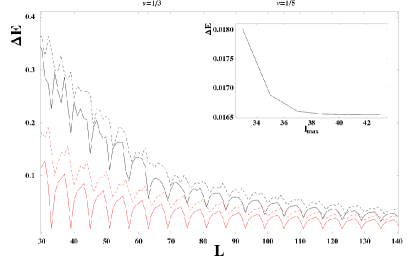
Figure 2: Dependence of the ground state energy (solid lines) and the first excites state energy (dashed lines) on the total angular momentum in the case of seven particles interacting with the Coulomb interaction. The black lines (red lines) show the energy difference between the result of the exact diagonalization (model Hamiltonian (8)) and the energy of the rigid rotation of the classical Wigner molecule. The upper panel is for bosons the lower panel for fermions. The inset shows the energy convergence as a function of the cut-off angular momentum of the LLL single particle basis in the case of fermions with $L=123$.

Once we have the energies and the symmetry properties of the classical vibrations solved, we need to quantize them to get the rotational spectrum of Eq. (8). Determination of the symmetry properties means that for fermions we demand that the quantized state is antisymmetric and for bosons symmetric.

Figure 2 demonstrates how the quantum mechanical spectrum approaches to that obtained by quantizing the classical vibrations. The figure shows the lowest (so-called yrast state) and second lowest energy for each angular momentum. The energies are shown as the energy difference from the classically determined rotational energy, Eq. (8) with $n_{k}=n_{\rm CM}=0$.

The results show the characteristic oscillation as a function of the angular momentum. The oscillation can be understood as a rigid rotation of the ’molecule’ of localized particles. The symmetry properties allow only every sixth angular momentum due to the six-fold symmetry of the hexagon. For bosons the allowed angular momenta are $L=6n$ and for fermions $L=6n+3$, where $n$ is an integer. For angular momenta in between, the purely rotational state has to be accompanied by a vibrational state, and consequently the energy is higher.

Figure 2 shows that already from angular momentum of about $L=40$, corresponding to filling factor $\nu=1/2$, the model Hamiltonian (8) describes qualitatively well the oscillations of the energy as a function of the angular momentum, when compared to the results of diagonalization of the Hamiltonian (3). The agreement gets better with increasing angular momentum. Naturally, the spectra for fermions and bosons become then identical, apart of a phase shift dictated by the symmetry requirements.

The reason that at high angular momenta the absolute energies of the exact diagonalization remains higher than those of the model Hamiltonian is due to the anharmonicity of the classical vibration potential: The zero point energy contribution coming from the high energy modes of Fig. 1 causes the energy shift (i.e. the zero-point energy is underestimated due to the harmonic approximation). The restriction of the basis within the lowest Landau level or the cut-off used for large angular momenta do not play any marked role. The inset in Fig. 2 shows the dependence of the energy on the cut-off single particle angular momentum for $L=123$. Note the different energy scale and that the total energy indeed depends very little on the cut-off angular momentum.

Figure 3 shows in more detail part of the low energy spectrum for seven electrons calculated by two different ways, quantum mechanically and classically. We remind that in both cases the values are for interaction energy i.e $\Delta E=E-(N+L)\hbar\omega_{0}$, where $E$ is either the solution from the diagonalization of the quantum mechanical Hamiltonian (3) or the classical energy (8). In Fig. 3 the classical spectrum is shifted up by a constant energy (0.014 a.u.) to make the comparison of the structure of the spectra easier. We can see that the two spectra agree in all details. Note also that the difference in the interaction energy given by the two models, $0.014/2.60\approx 0.5\%$, is very small indeed.

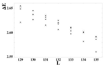
Figure 3: Low energy spectrum of seven electrons at high angular momenta. Black dots show the exact diagonalization results and open squares the results of the model Hamiltonian (8), shifted upwards with a constant 0.014. $\Delta E$ is the interaction energy in atomic units ($\omega_{0}=0.5$). The ground states for $L=129$ and 135 are purely rotational states. The ground states from $L=130$ to $L=134$ have vibrational modes $\omega_{5}$, $\omega_{4}$, $\omega_{6}$, $\omega_{7}$, $\omega_{3}$, respectively.

The oscillatory behavior of the results presented in Figs. 2 and 3 is not surprising since similar results were reported by Maksym maksym1996 ; maksym2000 for three, four, five and six electrons in a quantum dot. Here we have shown that similar spectrum is obtained for fermions and bosons and the approach to the classical limit is similar in both cases.

Finally, we would like to note that in the case of seven particles the classical geometry of a seven-fold ring is also stable. However, its energy is so much higher that it does not have any contribution to the low energy spectrum at any angular momenta. The situation is different to that of six particles, where the ground state of a five-fold ring (with a particle at the center) and the six-fold ring are very close in energy and both contribute to the rotational spectrummaksym1996 ; manninen2001 . Nevertheless, at higher energies the seven-fold ring also exists. As an example, Fig. 4 shows the pair correlation function of the $17^{\text{th}}$ state at $L=133$. Clearly, it shows seven particles in a ring with an empty center.

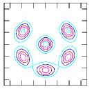
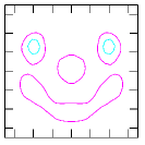
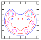
Figure 4: Pair correlation functions for selected states of seven electrons. Left panel shows the purely rotational state (ground state for $L=117$). The center panel shows a vibrational state (fourth excited state for $L=133$), which consists of vibrational modes $\omega_{5}$ and $\omega_{6}$. The right panel shows a seven-fold ring as a high excited state (17th state for $L=133$).

III.2 Gaussian interparticle interaction

In order to study the effect of the range of the interparticle interaction to the localization of particles we used Gaussian potential, Eq. (2). In this case we study a rather simple case of four particles. The ground state classical configuration of four particles is a square. Prus et alprus2004 have developed a model that considers electrons as Gaussian probability densities. They showed that this model yields also to the formation of a Wigner molecule. At this point we want to stress that our model is different from that because here the particles are point like but the interaction between the particles is Gaussian. Solving the eigenmodes is a bit more tricky than it was with the Coulomb interaction because the form of the interparticle interaction leads into transcendent equations at some point. As in the case of Coulombic interaction, knowing the modes is important, because the symmetry properties of the mode define all the allowed combinations of angular momenta and vibrational modes. In the three particle situation this point is reached at the end of the calculations so that it is easy to keep accounts for which energy value belongs to which mode. The four particle problem, however, is somewhat more troublesome because the stage of transcendent equations comes before the diagonalization of the dynamical matrix. This leads to difficulties of keeping track of eigenmodes and eigenergies for different angular momenta. We solved this problem by writing a program that finds out the right mode for a certain eigenenergy for every angular momentum separately.

Due to the symmetry, the vibrational modes are identical with the modes obtained in maksym1996 ; nikkarila2007 with Coulombic interparticle interaction, and consequently their symmetry properties are known from the previous reports maksym1996 ; nikkarila2007 . In the rotating frame the four particles have two low-energy modes. In the case of Gaussian interaction these two modes cross each other when the angular momentum is increased. The angular momentum where this happens depends on the width $\sigma$ of the Gaussian potential. This as such is interesting, and if the classical model describes the behavior of the quantum mechanical system correctly, the same phenomenon should also occur in the quantum mechanical spectrum. We will return to this detail later after we have presented the results for quantum mechanical systems and the corresponding classical systems.

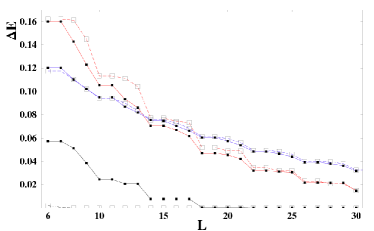
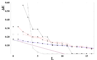
Figure 5: Interaction energy for four fermions (uper panel) and four bosons (lower panel) as a function of the angular momentum, calculated using different widths $\sigma$ of the Gaussian interaction. Black dots connected with solid lines show the results of the exact diagonalization in the LLL and the open circles connected with dashed lines the results of the model Hamiltonian (8). Red curves, $\sigma=3.0$; blue curves, $\sigma=2.0$; black curves; $\sigma=0.5$. The solid black and red lines (without points) show the exact and model Hamiltonian results for a harmonic interparticle interaction.

The quantum mechanical and classical energies for Gaussian repulsion in the case of four fermions and bosons are represented in Fig. 5 for three different values of $\sigma$: $0.5$, $2$ and $3$. The results show that the behavior of the quantum mechanical systems approach to the behavior of corresponding classical systems when the Gaussian interparticle potential is broadened from a nearly contact potential into a smoother potential. When $\sigma=3$, the quantum mechanical spectrum is nearly identical with the corresponding classical spectrum. When $\sigma$ is decreased the classical and quantum mechanical results start to depart, although the similar structure survives until very small values of $\sigma$.

Figure 5 also shows the results for a delta-function interaction ($\sigma=0$) and for a repulsive harmonic interaction ($v(r)=1/(\pi\sigma^{2})(1-r^{2}/\sigma^{2})$, with $\sigma=3$). In the case of the delta function interaction the interaction energy of the classical system is zero while the quantum mechanical particles feel each other up to Laughlin states where the contact interaction disappears, i.e. up to $L=N(N-1)/2$ for fermions and $L=N(N-1)$ for bosons. Beyond these angular momenta, the quantum mechanical and classical energies trivially agree. At this point it is interesting to note that in quasi-one-dimensional quantum rings of fermions, where the spectrum is dominated by particle localization at all angular momenta, even a delta function interparticle interaction leads to vibrational statesviefers2004 .

In the case of the repulsive harmonic interaction, Eq. (5), the classical result approaches fast the quantum mechanical result when $\lambda$ increases, as seen from Eqs. (6) and (10). Figure 5 show results for the value $\lambda$ corresponding to the leading term of Gaussian interaction with $\sigma=3.0$. In this case the classical and quantum mechanical results follow the same line shown in the figures. Since the classical approach gives correct results in the delta function limit and for the wide Gaussian limit it is not surprising that it describes the quantum mechanical spectra nearly exactly for all values of $\sigma$ when $L>N(N-1)$.

We have also made similar systematic study for three particles and limited computations for seven particles using the Gaussian interactions. The results are qualitatively similar to those presented here for four particles.

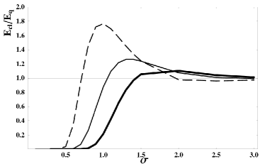
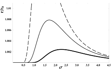
Figure 6: Upper panel: Ratio of the ground state energy of the classical model Hamiltonian and the exact diagonalization energy $E_{\text{cl}}/E_{\text{q}}$ as a function of the width of the Gaussian interaction $\sigma$. Lower panel: Radius $r$ of the classical equilibrium polygon (a square) as a function of $\sigma$. $r_{0}$ is the radius for $\sigma=0$). Dashed lines are for angular momentum $L=6$, solid lines for $L=10$ and the thick solid lines for $L=18$.

The classical model seems to describe very well the quantum mechanical system especially at higher values of $\sigma$. In figure 6 we present a more detailed study of the effect of $\sigma$ to the energy spectra. On the upper panel we present the ratio of classical and the quantum mechanical ground state energies as a function of $\sigma$ for a few fixed angular momenta. On the other hand the results of the lower panel show how the radius of the classical equilibrium polygon (i.e a square) depends on the value of $\sigma$. The radii are normalized to one for every angular momenta when $\sigma\approx 0$ in order to draw the different radii on the same picture. The behavior of the radii means that for a fixed angular momentum the equilibrium configuration (i.e a square) first expands as a function of $\sigma$ until it reaches its maximum value, and after that starts to shrink. The results on the two figures show a significantly similar behavior of the two variables as a function of $\sigma$. The explanation of such similarity is that classical particles do not feel each others at all if the Gaussian potential is steep. When the potential broadens the potentials of different particles start to overlap. Quantum mechanical particles on the other hand feel each others even if the interparticle potential is a point contact (i.e $\sigma\approx 0$).

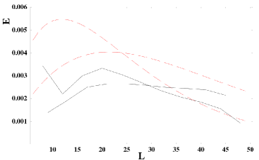
Figure 7: Dependence of the two low-energy vibrational modes on the total angular momentum in the case of four fermions interacting with a Gaussian interaction with $\sigma=3.0.$ Dashed red lines show the classical results and solid black lines the quantum mechanical results from the exact diagonalization.

We will now return to the crossing of the energies of the two lowest vibrational modes, when the angular momentum increases. The symmetry dictates that one of these modes is the lowest energy state at angular momenta $L=4n$ in the case of fermions ($L=4n+2$ for bosons) and the other mode at angular momenta $L=4n+1$ for fermions ($L=4n+3$ for bosons). In order to get an estimate of the vibrational energy from the exact diagonalization we have to subtract from the total interaction energy the energy of the rigid rotation. This we have estimated by fitting a smooth function of angular momentum through the energies of the purely rotational states $L=6,10,14,\cdots$ for fermions. The resulting vibrational energies for the Gaussian width $\sigma=3.0$ are plotted in Fig. 7, together with the classical vibrational energies, as a function of the angular momentum. The results show that both classical and quantum mechanical vibrational energies cross each other at about the same angular momentum. This finding supports the previous notions that the properties of the quantum mechanical system of a few particles rotating in a harmonic confinement can be explained with finest details by a model of vibrating molecule of localized particles.

Figure 8: Average radius of the ring of four bosons as a function of the angular momentum $L$, calculated with exact diagonalization in the LLL. The center line and points show the radius $R$ and the lower and upper lines and points $R\pm W$, where $W$ is the variance of the radius. Solid lines show results for the Gaussian interaction with $\sigma=3.0$, squares for $\sigma=0.05$ and crosses for the Coulomb interaction. Dotted line is the result for classical particles with Gaussian interaction, $\sigma=3.0$.

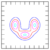
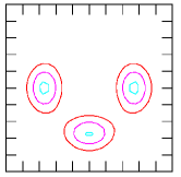
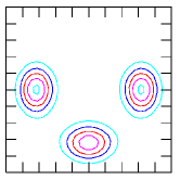
Figure 9: Pair correlation functions of four fermions interacting with the Gaussian interaction with $\sigma=3.0$. Upper row shows results for $L=10$ (left)and $L=18$ (right) and the lower row for $L=30$ (left) and $L=42$ (right). The contour plots are in the same scale to demonstrate the expansion due to the rotation.

Finally, we would like to quantify the degree of localization in the quantum mechanical many-particle system. The symmetry of the Hamiltonian dictates that the total particle density is circularly symmetric. However, for small number of particles they localize in circles and consequently the radial density distribution gives direct information of the degree of localization. In the case of four electrons we have determined the average radius $R$ of the ring of electrons and its variance $W$, which describes the width of the localized electron state:

$$R=\frac{1}{N}\int d{\bf r}r\rho(r),\quad W^{2}=\frac{1}{N}\int d{\bf r}(r-R)^{2}\rho(r),$$ (11)

where $\rho$ is the total electron density. It turns out that for the quantum mechanical system both the radius and its variance are nearly independent of the shape or strength of the interparticle interaction. The results for bosons are shown in Fig. 8 as a function of the angular momentum. The radius reaches fast the classical value and it is nearly independent of the interparticle interaction. Similarly the width is independent of the interaction and also nearly constant as a function of the angular momentum. The increased localization is mainly due to the increase of the radius with $L$ which makes the relative width to decrease.

The same result is seen qualitatively in Fig. 9 where the pair correlation function for four fermions with Gaussian interaction ($\sigma=3.0$) is shown for four different values of the angular momentum. The pair correlation function demonstrates that the angular localization increases with the same rate as the radial localization.

III.3 Rotation in a 3D harmonic confinement

Above we have considered rotational spectra of interacting particles in a 2D harmonic potential. In the 3D case the classical particles interacting with repulsive interation tend to form spherical shellsmanninen1986 . However, when put into rotation, it is energetically favorable for the 3D structure to collapse into a 2D structure due to the increased momentum of inertia. For small number of particles this happens already at small angular momenta.

As an example we have studied the case of seven particles interacting with Coulomb interaction. The ground state geometry of a nonrotating system is a pentagonal bipyramid, i.e. a five-fold ring in the $x$-$y$-plane with two atoms at positions $\pm c\hat{z}$. When this is put in rotation the five-fold ring will expand while the particles in the $z$ axis will get closer to each other. However, already at angular momentum $L=7$ the planar hexagon with one particle at the center will have lower energy and at angular momentum $L=8$ the energy difference between the 3D and 2D structures is much larger than the vibrational energies of the 2D structure.

Similar results are obtained for other small particle numbers in 3D harmonic oscillator. Consequently, we can safely state that the region where the classical model explains the spectrum for the 2D harmonic oscillator the result would be the same had we done the computations for the 3D confinement.

IV Conclusions

We have studied the rotation induced localization of particles, in a two-dimensional circular harmonic trap. Earlier studies have already shown that a long-range Coulomb interaction causes formation of Wigner molecules in quantum dots and that the quantum mechanical many-particle spectra can be determined by canonical quantization of the rigid rotation and vibrational modes of the moleculemaksym1996 ; nikkarila2007 . The present calculations show that Coulomb interaction also causes similar localization of bosonic particles. For seven particles (fermions or bosons) the low energy rotational spectrum is determined by vibrational modes of the molecule already before the angular momentum corresponding to the filling factor $\nu=1/2$ of the quantum Hall liquid is reached.

For mimicking atoms in a harmonic traps we have used Gaussian interparticle interaction and studied the dependence of the localization on the range of the interaction. It was observed that both in the short range (delta function) and long range (repulsive harmonic) limit the classical model gives exactly the quantum mechanical energies. Consequently, for any range of Gaussian interaction the classical model describes very accurately the quantum mechanical many-particle energy spectrum at large enough angular momenta. However, the delta function interaction does not support particle localization (particles do not feel each other).

We also estimated that in a three-dimensional harmonic confinement the rotating particles form very fast a two-dimensional configuration. For example, for seven particles with Coulomb interaction this happens already at $L=7$, meaning that in the 3D confinement the low-energy rotational spectrum agrees with that calculated for a 2D system.

In conclusion, independent of the form of the repulsive interparticle interaction or the type of the particles, the rotational spectrum of the particles confined in a harmonic trap can be estimated by quantizing the classical vibrational modes determined for localized particles in a rotating frame.

Acknowledgments

We would like to thank Stephanie Reimann for valuable discussions. This work was supported by the Academy of Finland and by the Jenny and Antti Wihuri Foundation.

References

- (1) S. Tarucha, D.G. Austing, T. Honda, R.J. van der Hage, and L.P. Kouwenhoven, Phys. Rev. Lett. 77, 3613 (1996).
- (2) P.L. McEuen, E.B. Foxman, U. Meirav, M.A. Kastner, Y. Meir, N.S. Wingreen and S.J. Wind, Phys. Rev. Lett. 66, 1926 (1991).
- (3) T.H. Oosterkamp, J.W. Janssen, L.P. Kouwenhoven, D.G. Austing, T. Honda, and S. Tarucha, Phys. Rev. Lett. 82, 2931 (1999).
- (4) A.H. MacDonald, S.R.E. Yang, and M.D. Johnson, Aust. J. Phys. 46, 345 (1993).
- (5) R.B. Laughlin, Phys. Rev. B 27, 3383 (1983).
- (6) P.A. Maksym and T. Chakraborty, Phys. Rev. Lett. 65, 108 (1990).
- (7) A. Wójs and P. Hawrylak, Phys. Rev. B 56, 13227 (1997).
- (8) P.A. Maksym, Phys. Rev. B 53, 10871 (1996).
- (9) K.W. Madison, F. Chevy, W. Wohlleben, J. Dalibard, Phys. Rev. Lett. 84, 806 (2000).
- (10) J.R. Abo-Shaer, C. Raman, J.M. Vogels, and W. Ketterle, Science 292, 476 (2001)
- (11) M. W. Zwierlein, J. R. Abo-Shaeer, A. Schirotzek, C. H. Schunck and W. Ketterle, Nature 435, 1047 (2005).
- (12) M. Koskinen, M. Manninen, and S.M. Reimann, Phys. Rev. Lett. 79, 1389 (1997).
- (13) S.M. Reimann, Koskinen, M., Manninen, M., and Mottelson, B.R., Phys. Rev. Lett. 83, 3270 (1999).
- (14) H. Saarikoski, A. Harju, M. J. Puska, and R. M. Nieminen, Phys. Rev. Lett. 93, 116802 (2004).
- (15) M. Manninen, S. M. Reimann, M. Koskinen, Y. Yu and M. Toreblad, Phys. Rev. Lett. 94, 106405 (2005).
- (16) H.M. Muller and S.E. Koonin, Phys. Rev. B 54, 14532 (1996).
- (17) C. Yannouleas, and U. Landman, Phys. Rev. Lett. 82, 5325 (1999).
- (18) S.M. Reimann, M. Koskinen, and M. Manninen, Phys. Rev. B 62, 8108 (2000).
- (19) D.A. Butts and D.S. Rokhsar Nature 397, 327 (1999).
- (20) B. Mottelson, Phys. Rev. Lett. 83, 2695 (1999).
- (21) G.F. Bertsch and T. Papenbrock, Phys. Rev. Lett. 83, 5412 (1999).
- (22) M. Toreblad, M. Borgh, M. Koskinen, M. Manninen, and S. M. Reimann, Phys. Rev. Lett. 93, 090407 (2004).
- (23) S. M. Reimann, M. Koskinen, Y. Yu, and M. Manninen Phys. Rev. A 74, 043603 (2006).
- (24) M. Manninen, S. Viefers, M. Koskinen, and S.M. Reimann, Phys. Rev. B 64, 245322 (2001).
- (25) I. Romanovsky, C. Yannouleas, L.O. Baksmaty, and U. Landman, Phys. Rev. Lett. 97, 090401 (2006).
- (26) S.M. Reimann, M. Koskinen, Y. Yu, and M. Manninen New Journal of Physics, 8, 59 (2006).
- (27) A.D. Güçlü, Gun Sang Jeon, C.J. Umrigar and J.K. Jain, Phys. Rev. B. 72, 205327 (2005).
- (28) R.D. Lawson, Theory of Nuclear Shell Model, (Oxford Press, Oxford 1980).
- (29) N.F. Johnson, Phys. Rev. B 46, R2636 (1992).
- (30) V. Ruuska and M. Manninen, Phys. Rev. B 72, 153309 (2005).
- (31) J.K. Jain, Phys. Rev. Lett.”, 63, 199 (1989).
- (32) J.K. Jain, Phys. Rev. B 41, 7653 (1990).
- (33) G.S. Jeon, C.-C. Chang, and J.K.Jain, Phys. Rev. B 69, 241304(R) (2004).
- (34) F. Bolton and U. Rößler, Superlatt. Microstr. 13, 139 (1993).
- (35) V.M. Bedanov and F.M. Peeters, Phys. Rev. B 49, 2667 (1994).
- (36) P.A. Maksym, Europhys. Lett. 31, 405 (1995).
- (37) H. Goldstein, Classical Mechanics (Adison-Wesley, Reading 1969).
- (38) N.W. Ashcroft and N.D. Mermin, Solid State Physics (Saunders College, Philadelphia 1976).
- (39) M. Tinkham, Group theory and quantum mechanics (McGraw-Hill, New York 1964).
- (40) W.Y. Ruan, Y.Y. Liu, C.G. Bao, and Z.Q. Zhang, Phys. Rev. B 51, 7942 (1995).
- (41) M. Koskinen, M. Manninen, B. Mottelson, and S.M. Reimann, Phys. Rev. B 63, 205323 (2001)
- (42) P. Koskinen, M. Koskinen, and M. Manninen, Eur. Phys. J B 28, 483 (2002).
- (43) P.A. Maksym, H. Imamura, G.P. Mallon, and A. Aoki, J. Phys. Cond. Mat. 12, R299 (2000).
- (44) A. Matulis and E. Anisimovas, J. Phys. Cond. Mat. 17, 3851 (2005).
- (45) J.-P. Nikkarila and M. Manninen, Solid State Commun. 141, 209-213 (2007).
- (46) V.A. Schweigert, F.M. Peeters, Phys. Rev. B 51, 7700 (1995).
- (47) T. Prus, B. Szafran, J. Adamowski and S. Bednarek, J. Phys. Cond. Mat. 16, 1425-1437 (2004).
- (48) M. Manninen, Solid State Commun. 59, 281 (1986).
- (49) S. Viefers, P. Koskinen, P. Singha Deo, and M. Manninen, Physica E 21, 1 (2004).