Three-particle collisions in quantum wires:
Corrections to thermopower and conductance

Abstract

We consider the effect of electron-electron interaction on the electron transport through a finite length single-mode quantum wire with reflectionless contacts. The two-particle scattering events cannot alter the electric current and therefore we study the effect of three-particle collisions. Within the Boltzmann equation framework, we calculate corrections to the thermopower and conductance to the leading order in the interaction and in the length of wire $L$. We check explicitly that the three-particle collision rate is identically zero in the case of several integrable interaction potentials. In the general (non-integrable) case, we find a positive contribution to the thermopower to leading order in $L$. The processes giving rise to the correction involve electron states deep in the Fermi sea. Therefore the correction follows an activation law with the characteristic energy of the order of the Fermi energy for the electrons in the wire.

I Introduction

Short clean one-dimensional (1D) mesoscopic wires, often referred to as quantum point contacts, show conductance quantizationWees1988 ; Wharam1988 as a function of the channel width. The quantization is well described by the theory of adiabatic propagation of free electrons.GlazmanJETPlett1988 For non-interacting particles, conductance quantization should occur in longer channels too, as long as there is no backscattering off inhomogeneities within the channel.

A lot is known about the role of electron-electron interaction of 1D channels. Electron-electron repulsion in a wire enhances dramatically the reflection coefficient, making it energy-dependent.chang-review1D-2003 However, interaction between electrons does not alter the quantization (in units of $2e^{2}/h$) of an ideal channel conductance in the limit of zero temperature.fisherglazman97 ; Maslov2004 What is still an open question is whether there are other manifestations of interactions due to inelastic processes, which influence the transport properties.

In the absence of interactions, left- and right-moving particles in a wire are at equilibrium with the reservoirs they originate from. If a bias is applied between the reservoirs, then these equilibria differ from each other, giving rise to a particular form of the non-equilibrium distribution inside the channel. On the other hand, in a long ideal channel and in the presence of interactions one may expect equilibration to occur between the left- and right-movers into a single distribution characterized by an equilibrium with respect to a reference frame moving with some drift velocity. Interestingly, in a model with momentum-independent electron velocity for left- and right-movers (as it is the case in Tomonaga-Luttinger model) there is no difference between the two distributions. Effects originating from the particle-hole asymmetry, however, may discriminate between the two. Thermopower and Coulomb drag Mortensen2001 ; Pustilnik-drag-2003 ; Flensberghcis1996 are examples of such effects.

Figure 1: A schematic picture of two metallic gates depleting the underlaying two dimensional electron gas and thereby forming a short 1D quantum wire of length $L$. This fabrication method has the advantage of producing reflectionless contacts to the leads,GlazmanJETPlett1988 so that the boundary conditions of the distribution function is given by the Fermi function of the reservoirs. We define the thermopower as $S=V/\Delta T\big{|}_{I=0}$, i.e. the voltage $V$ required to counteract a current due to the temperature difference $\Delta T$.

At present, little is known about equilibration in a 1D electron system. In higher dimensions the electron-electron interaction provides the most effective relaxation mechanism at low temperatures and therefore we include this relaxation mechanism as the first approach. However, in 1D pair collisions cannot change the distribution function for quadratic dispersion, since the momentum and energy conservationfootnote-pair-scattering-one-band laws result in either zero momentum exchange or an interchange of the two momenta. sutherland In either case the distribution function remains the same. Thus, the leading equilibration mechanism is due to three-particle collisions, which we study in this paper.khodasCM0702505

We investigate here the effects of three-particle collisions in reasonably short wires (see Fig. 1), where electron-electron scattering can be considered perturbatively. As measurable quantities, we evaluate the temperature dependence of the thermopower and conductance. Note that for more than one mode pair collisions become important for certain fillings.Lunde-Flensberg-Glazman-2006

The paper is organized as follows: First we review the non-interacting limit of thermopower and give a qualitative explanation of the effects due to three-particle collisions. Then we describe how to include the electron interactions using the Boltzmann equation. Next we calculate the main ingredient for our perturbation theory, namely the three-particle matrix element and scattering rate using a $T$-matrix expansion. We note several interesting properties of this scattering rate. Finally, we derive the conductance and thermopower corrections and discuss the deviation from the so-called Mott formula. Furthermore, some technical details are put in two appendices, and in Appendix A we show that the number of left and right movers have to change in a scattering event for the current to change.

I.1 Thermopower in the non-interacting limit

For a wire without interactions the distribution function $f^{(0)}$ is determined solely by the electron reservoirs

$$f_{k}^{(0)}=\left\{\begin{array}[]{ll}f^{0}(\varepsilon_{k}\!-\!\mu_{\textrm{L}},T_{\textrm{L}})\equiv f^{0}_{\textrm{L}}(\varepsilon_{k})&\textrm{for}\ k>0,\\ f^{0}(\varepsilon_{k}\!-\!\mu_{\textrm{R}},T_{\textrm{R}})\equiv f^{0}_{\textrm{R}}(\varepsilon_{k})&\textrm{for}\ k<0,\\ \end{array}\right.$$ (3)

where $\varepsilon_{k}$ is the dispersion relation for momentum $k$ and spin $\sigma$ (suppressed in the notation), and $f^{0}(\varepsilon-\mu,T)=[1+\exp((\varepsilon-\mu)/k_{\textrm{B}}T)]^{-1}$ is the Fermi function with $\mu_{\rm L/R}$ and $T_{\rm L/R}$ denoting the chemical potential and temperature of the left/right contact, respectively (see Fig. 1). The electric current for low temperature $T\ll T_{\textrm{F}}$ and in linear response to the applied bias $V$ and temperature difference $\Delta T\ll T$ then follows as ($e>0$)MolenkampSSAT1992

$$I^{(0)} =\frac{(-e)}{L}\sum_{\sigma k>0}v_{k}\left(f^{0}_{\textrm{L}}(\varepsilon_{k})-f^{0}_{\textrm{R}}(\varepsilon_{k})\right)$$ (4)

$$\simeq-\frac{2e^{2}}{h}V\left(1-e^{-T_{\textrm{F}}/T}\right)+\frac{2e}{h}k_{\textrm{B}}\Delta T\frac{T_{\textrm{F}}}{T}e^{-T_{\textrm{F}}/T}.$$ (5)

From this the well-known leading-order results for conductance

$$G^{(0)}=\frac{2e^{2}}{h}\left(1-e^{-T_{\textrm{F}}/T}\right)$$ (6)

and for thermopower

$$S^{(0)}=\frac{k_{\textrm{B}}}{e}\frac{T_{\textrm{F}}}{T}e^{-T_{\textrm{F}}/T}$$ (7)

for a fully open channel are obtained. Here $T_{\textrm{F}}\equiv\varepsilon_{\textrm{F}}/k_{\textrm{B}}$ is the Fermi temperature.

I.2 Main results and a simple picture of the effect of the three-particle scattering

Figure 2: (a) The dominant three-particle scattering process at low temperature in a single energy band. (b) The three-particle scattering process perturbing the initial distributions shown with warm left moving electrons ($k<0$) and cold right moving electrons ($k>0$). Due to the temperature difference of the initial distributions the scattering process creating left movers dominate compared to the opposite scattering and therefore it gives a positive correction to the thermopower.

One of the main results of this paper is that the three-particle collisions give a positive contribution to the thermopower, i.e. the current due to a temperature difference is increased by the three-particle scattering. This can be explained in simple terms. Firstly, to change the current the number of left and right moving electrons need to change, since it is the number of electrons going through a mesoscopic structure that determines the current and not their velocity (see the Appendix A). Secondly, we find the dominant scattering process at low temperature to only involve a single electron changing direction. This occurs near the bottom of the band as pictured on Fig. 2(a). For the initial electronic distribution the left moving electrons have a higher temperature then the right moving ones, which favors scattering into the warmer distribution as seen on Fig. 2(b). This thus creates more left moving electrons and thereby increases the particle current towards the colder reservoir, i.e. increasing the thermopower.

Another important point is that the thermopower and conductance corrections are exponential in temperature, i.e. proportional to $\exp(-T_{\textrm{F}}/T)$. This is a direct consequence of the dominant three-particle scattering process requiring an empty state near the bottom of the band. We find the form of the thermopower correction at low temperatures due to the three particle scattering to be given by

$$S^{\textrm{int}}\propto L|V|^{4}\left(\frac{T}{T_{\textrm{F}}}\right)^{6}\exp(-T_{\textrm{F}}/T)>0,$$ (8)

where $V$ is the electron-electron interaction strength and $T_{\textrm{F}}$ the Fermi temperature. This is found perturbatively in the short wire limit. The long-wire limit remains an open question, and we expect that the length dependence of thermopower saturates once $L$ exceeds some relaxation length (which increases for decreasing temperature).

In contrast, the conductance correction is negative. To understand this, note that the chemical potential of the initial distribution is higher for the right moving electrons then the left moving ones. This favors scattering into the left moving branch (still with the process shown in Fig. 2(a)) for non-zero temperature and thereby decreasing the current. The form of the conductance correction is similar to the thermopower correction:

$$G^{\textrm{int}}\propto-L|V|^{4}\left(\frac{T}{T_{\textrm{F}}}\right)^{7}\exp(-T_{\textrm{F}}/T)<0.$$ (9)

II Current calculation in the Boltzmann equation formalism

II.1 Effect of interactions on the current

To model the current through a short 1D quantum wire including perturbatively the three particle interactions, we use the Boltzmann equation

$$v_{k}\partial_{x}f_{k}(x)=\mathcal{I}_{kx}[f],$$ (10)

where $f_{k}(x)$ is the distribution function at a space point $x$ between zero and $L$ (see Fig. 1), $v_{k}=\frac{1}{\hslash}\partial_{k}\varepsilon_{k}$ is the velocity and $\mathcal{I}_{kx}[f]$ is the three-body electronic collision integral, i.e. no impurity or interface roughness effects are included here. We include the voltage and temperature difference in the boundary conditions of the reflectionless contacts,GlazmanJETPlett1988 i.e.

$$f_{k}(x=0) =f^{0}_{\textrm{L}}(\varepsilon_{k})\quad\textrm{for}\quad k>0,$$ (11a)

$$f_{k}(x=L) =f^{0}_{\textrm{R}}(\varepsilon_{k})\quad\textrm{for}\quad k<0,$$ (11b)

and therefore omit the term $\dot{k}\partial_{k}f_{k}(x)$ in the Boltzmann equation, allowed in the linear response regime.Sharvin1965 A similar method has been used to investigate electron-phonon interactions in short quantum wires,GurevichPRB1995 quantum Hall effect in quantum wires AndoPRB1990 and ballistic Coulomb drag.GurevichJPCM1998

The three-particle collision integral is assumed to be local in space and is given by

$$\mathcal{I}_{k_{1}x}[f]= -\!\!\!\!\!\!\sum_{\begin{subarray}{c}\sigma_{2}\sigma_{3}\\ \sigma_{1^{\prime}}\sigma_{2^{\prime}}\sigma_{3^{\prime}}\end{subarray}}\sum_{\begin{subarray}{c}k_{2}k_{3}\\ k_{1^{\prime}}k_{2^{\prime}}k_{3^{\prime}}\end{subarray}}\!\!\!\!W_{123;1^{\prime}2^{\prime}3^{\prime}}\left[f_{1}f_{2}f_{3}(1-f_{1^{\prime}})(1-f_{2^{\prime}})(1-f_{3^{\prime}})-f_{1^{\prime}}f_{2^{\prime}}f_{3^{\prime}}(1-f_{1})(1-f_{2})(1-f_{3})\right],$$ (12)

where the quantum numbers are primed/unprimed after/before the scattering event, $f_{i}\equiv f_{k_{i}}(x)$ and the scattering rate $W_{123;1^{\prime}2^{\prime}3^{\prime}}$ is found in the next section. Without interactions ($W_{123;1^{\prime}2^{\prime}3^{\prime}}=0$) the solution of the Boltzmann equation is simply given by $f^{(0)}$ in Eq. (3). When interactions are included it becomes a very difficult task to solve the Boltzmann equation to all orders in the interaction. However, for a short wire the interactions only have short time to change the distribution function away from the initial distribution $f^{(0)}$ and therefore we expand the distribution function in orders of $W_{123;1^{\prime}2^{\prime}3^{\prime}}$ as

$$f=f^{(0)}+f^{(1)}+\cdots.$$ (13)

To find $f^{(1)}$ to the first order in $W$, we insert the expansion of $f$ in the Boltzmann equation and realize that only $f^{(0)}$ is necessary in the collision integral. Since $\mathcal{I}_{kx}[f^{(0)}]=\mathcal{I}_{k}[f^{(0)}]$ is independent of $x$, we find that

$$f_{k}^{(1)}(x) =\frac{x}{v_{k}}\mathcal{I}_{k}[f^{(0)}]\quad k>0,$$ for (14a)

$$f_{k}^{(1)}(x) =\frac{x-L}{v_{k}}\mathcal{I}_{k}[f^{(0)}]\quad k<0,$$ for (14b)

using the boundary conditions Eq. (11). Therefore the current to the first order in $W$ is

$$I=I^{(0)}+e\sum_{\sigma k<0}\mathcal{I}_{k}[f^{(0)}]\equiv I^{(0)}+I^{\textrm{int}},$$ (15)

where $I^{(0)}$ is the non-interacting (Landauer) part of the current from Eq. (4) and $I^{\textrm{int}}$ is the part due to interactions.

II.2 The linear response limit

The form of the interacting part of the current is now known and the next step is therefore to evaluate it to linear response to $V$ and $\Delta T$ to obtain the thermopower and conductance corrections. To this end, we define $\psi_{k}^{(0)}$ via

$$f_{k}^{(0)}\equiv f^{0}(\varepsilon_{k})+f^{0}(\varepsilon_{k})(1-f^{0}(\varepsilon_{k}))\psi_{k}^{(0)},$$ (16)

where $f^{0}(\varepsilon_{k})$ is the Fermi function with temperature $T$ and Fermi level $\varepsilon_{\textrm{F}}$. It turns out that $\psi_{k}^{(0)}$ is proportional to either $V$ or $\Delta T$. This is seen by using the identity

$$-k_{\textrm{B}}T\partial_{\varepsilon}f^{0}(\varepsilon_{k})=f^{0}(\varepsilon_{k})(1-f^{0}(\varepsilon_{k})),$$ (17)

so we can identify $\psi_{k}^{(0)}$ by expanding the non-interacting distribution function $f^{(0)}_{k}$ (see Eq. (3) and Fig. 1)

$$f^{0}_{\textrm{L}}(\varepsilon_{k}) \simeq f^{0}(\varepsilon_{k})+\left[-\partial_{\varepsilon}f^{0}(\varepsilon_{k})\right]eV,$$ (18a)

$$f^{0}_{\textrm{R}}(\varepsilon_{k}) \simeq f^{0}(\varepsilon_{k})+\left[-\partial_{\varepsilon}f^{0}(\varepsilon_{k})\right](\varepsilon-\varepsilon_{\textrm{F}})\frac{\Delta T}{T},$$ (18b)

i.e.

$$\psi_{k}^{(0)}=\left\{\begin{array}[]{ll}\frac{eV}{k_{\textrm{B}}T},&\hbox{ for $k>0$}\\ \frac{\varepsilon_{k}-\varepsilon_{\textrm{F}}}{k_{\textrm{B}}T}\frac{\Delta T}{T},&\hbox{ for $k<0$}\\ \end{array}\right..$$ (21)

Therefore to get $I^{\textrm{int}}$ in linear response to $V$ and $\Delta T$, we linearized the collision integral $\mathcal{I}_{k}[f^{(0)}]$ Eq. (12) with respect to $\psi_{k}^{(0)}$ and insert it into $I^{\textrm{int}}$ Eq.(15) to obtain

$$I^{\textrm{int}} =(-e)\!\!\!\!\!\!\sum_{\begin{subarray}{c}\sigma_{1}\sigma_{2}\sigma_{3}\\ \sigma_{1^{\prime}}\sigma_{2^{\prime}}\sigma_{3^{\prime}}\end{subarray}}\sum_{\begin{subarray}{c}k_{1}<0,k_{2}k_{3}\\ k_{1^{\prime}}k_{2^{\prime}}k_{3^{\prime}}\end{subarray}}\Delta_{123;1^{\prime}2^{\prime}3^{\prime}}$$

$$\times\left[\psi_{1}^{(0)}+\psi_{2}^{(0)}+\psi_{3}^{(0)}-\psi_{1^{\prime}}^{(0)}-\psi_{2^{\prime}}^{(0)}-\psi_{3^{\prime}}^{(0)}\right],$$ (22)

where we defined

$$\Delta_{123;1^{\prime}2^{\prime}3^{\prime}}=\\ W_{123;1^{\prime}2^{\prime}3^{\prime}}\ f_{1}^{0}f_{2}^{0}f_{3}^{0}(1-f_{1^{\prime}}^{0})(1-f_{2^{\prime}}^{0})(1-f_{3^{\prime}}^{0}),$$ (23)

using the shorthand notation $\psi_{i}^{(0)}\equiv\psi_{k_{i}}^{(0)}$ and $f^{0}_{i}\equiv f^{0}(\varepsilon_{k_{i}})$. To linearize the collision integral and thereby the correction to the current due to interactions $I^{\textrm{int}}$, we have used the relation

$$f_{1}^{0}f_{2}^{0}f_{3}^{0}(1-f_{1^{\prime}}^{0})(1-f_{2^{\prime}}^{0})(1-f_{3^{\prime}}^{0})=\\ f_{1^{\prime}}^{0}f_{2^{\prime}}^{0}f_{3^{\prime}}^{0}(1-f_{1}^{0})(1-f_{2}^{0})(1-f_{3}^{0}),$$ (24)

valid at $\varepsilon_{1}+\varepsilon_{2}+\varepsilon_{3}=\varepsilon_{1^{\prime}}+\varepsilon_{2^{\prime}}+\varepsilon_{3^{\prime}}$.

Since $\psi_{i}^{(0)}$ is different for positive and negative $k_{i}$, we need to divide the summation in $I^{\textrm{int}}$ Eq. (22) into positive and negative $k$ sums, which gives $2^{5}=32$ terms. For this purpose, we introduce the notation

$$\sum_{\begin{subarray}{c}k_{1}<0,k_{2}>0,k_{3}<0\\ k_{1^{\prime}}>0,k_{2^{\prime}}>0,k_{3^{\prime}}<0\end{subarray}}\!\!\!(\cdot)\equiv\sum_{\begin{subarray}{c}-+-\\ ++-\end{subarray}}(\cdot),\quad\sum_{\begin{subarray}{c}\sigma_{1}\sigma_{2}\sigma_{3}\\ \sigma_{1^{\prime}}\sigma_{2^{\prime}}\sigma_{3^{\prime}}\end{subarray}}\!\!\!\!(\cdot)\equiv\sum_{\textrm{spin}}(\cdot),$$ (25)

and similarly for other combinations of the summation intervals. The 32 terms can be simplified to only three terms using energy conservation and symmetry properties of $\Delta_{123;1^{\prime}2^{\prime}3^{\prime}}$ in Eq. (23) under interchange of indices. There are pairwise exchanges of indices $\Delta_{123;1^{\prime}2^{\prime}3^{\prime}}=\Delta_{213;1^{\prime}2^{\prime}3^{\prime}}=\Delta_{123;1^{\prime}3^{\prime}2^{\prime}}$ etc. and interchanges between primed and unprimed indices, $\Delta_{123;1^{\prime}2^{\prime}3^{\prime}}=\Delta_{1^{\prime}2^{\prime}3^{\prime};123}$, using Eq. (24) and the fact that $W_{123;1^{\prime}2^{\prime}3^{\prime}}$ contains a matrix element squared. This leads to six terms. Furthermore, $\Delta_{123;1^{\prime}2^{\prime}3^{\prime}}$ is invariant under $k_{i}\rightarrow-k_{i}$ for all $i=1,2,3,1^{\prime},2^{\prime},3^{\prime}$ simultaneously due to time reversal symmetry, also seen explicitly from the form of $W_{123;1^{\prime}2^{\prime}3^{\prime}}$ (derived below). An example of how the simplifications occurs can be seen in Eq. (65). Thus we obtain the more compact result

$$I^{\textrm{int}} =2(-e)\sum_{\textrm{spin}}\sum_{\begin{subarray}{c}-++\\ +++\end{subarray}}\Delta_{123;1^{\prime}2^{\prime}3^{\prime}}\left[\frac{\Delta T}{k_{\textrm{B}}T^{2}}(\varepsilon_{1}-\varepsilon_{\textrm{F}})-\frac{eV}{k_{\textrm{B}}T}\right]$$

$$+4(-e)\sum_{\textrm{spin}}\sum_{\begin{subarray}{c}--+\\ +++\end{subarray}}\Delta_{123;1^{\prime}2^{\prime}3^{\prime}}\left[\frac{\Delta T}{k_{\textrm{B}}T^{2}}\left\{(\varepsilon_{1}-\varepsilon_{\textrm{F}})+(\varepsilon_{2}-\varepsilon_{\textrm{F}})\right\}-\frac{2eV}{k_{\textrm{B}}T}\right]$$

$$+3(-e)\sum_{\textrm{spin}}\sum_{\begin{subarray}{c}++-\\ +--\end{subarray}}\Delta_{123;1^{\prime}2^{\prime}3^{\prime}}\left[\frac{\Delta T}{k_{\textrm{B}}T^{2}}\left\{-(\varepsilon_{3}-\varepsilon_{\textrm{F}})+(\varepsilon_{2^{\prime}}-\varepsilon_{\textrm{F}})+(\varepsilon_{3^{\prime}}-\varepsilon_{\textrm{F}})\right\}-\frac{eV}{k_{\textrm{B}}T}\right],$$ (26)

where the definition of $\psi_{i}^{(0)}$ in Eq. (21) was inserted. An important point is that the number of positive/negative wave-vector intervals is not the same before and after the scattering. Therefore, we note that only scattering events that change the number of left and right moving electrons contributes to the interaction correction to the current. The origin of this is the cancellation of the velocity in the definition of the current and in the distribution functions (14).

This cancellation thus leads to an expression for the interaction correction to the current in Eq. (26) where all the in-going and out-going momenta enter on equal footing. In the Appendix A, we show that this is valid to all orders in perturbation theory. Due to this property and momentum conservation, there are no processes that alter the current possible near the Fermi level. Consequently, states far away from the Fermi level have to be involved in the scattering, which, as we will see, leads to a suppression of $I^{\textrm{int}}$ by a factor $\exp(-T_{\textrm{F}}/T)$. The distribution function on the other hand, can be changed by scattering processes near the Fermi level.

To identify the important processes we find in the next section the scattering rate $W_{123;1^{\prime}2^{\prime}3^{\prime}}$.

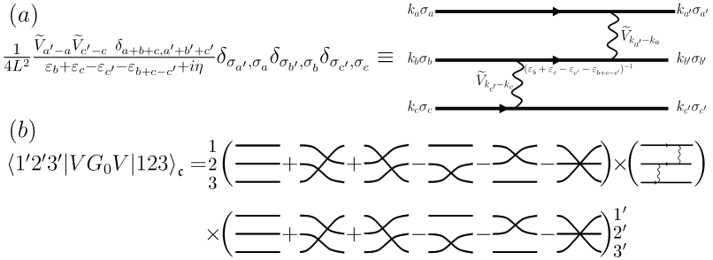
Figure 3: A visualization of the connected three-particle scattering matrix element Eq. (34), where three particles interchange their momenta and energy. This matrix element enters the scattering rate via the generalized Fermi Golden rule Eq. (27). (a) The basic three-particle interaction consisting of two interaction lines and a free propagation, see Eq. (34). (b) Picture of the exchange processes times the basic interaction needed to form the matrix element Eq. (34).

III Three-particle scattering rate

The three particle scattering rate $W_{123;1^{\prime}2^{\prime}3^{\prime}}$ is calculated using the generalized Fermi Golden rule inserting the $T$-matrix, $T\equiv V+VG_{0}T$, iterated to second order in the interaction $V$ to get the three particle interaction amplitude, i.e.,

$$W_{123;1^{\prime}2^{\prime}3^{\prime}}=\frac{2\pi}{\hslash}|\langle 1^{\prime}2^{\prime}3^{\prime}|VG_{0}V|123\rangle_{\mathfrak{c}}|^{2}\delta(E_{i}-E_{f}),$$ (27)

where $E_{i}=\varepsilon_{1}+\varepsilon_{2}+\varepsilon_{3}$ is the initial energy, $E_{f}=\varepsilon_{1^{\prime}}+\varepsilon_{2^{\prime}}+\varepsilon_{3^{\prime}}$ the final energy, $G_{0}$ is the resolvent operator (or free Green function), $j$ is short hand for $k_{j}$, and the subscript ’$\mathfrak{c}$’ means connected in the sense that the scattering process cannot be effectively a two particle process, where one of the incoming particles does not participate in the scattering. Explicitly $G_{0}$ and $V$ are given by

$$G_{0} =\frac{1}{E_{i}-H_{0}+i\eta},\qquad(\eta\rightarrow 0^{+})$$ (28)

$$V =\frac{1}{2L}\sum_{k_{1}k_{2}q}\sum_{\sigma_{1}\sigma_{2}}V_{q}c_{k_{1}+q\sigma_{1}}^{{\dagger}}c_{k_{2}-q\sigma_{2}}^{{\dagger}}c_{k_{2}\sigma_{2}}c_{k_{1}\sigma_{1}}.$$ (29)

Here $H_{0}$ is the unperturbed Hamiltonian (i.e. kinetic energy with some dispersion), $V_{q}$ the Fourier-transformed interaction potential, and $c_{k\sigma}$ ($c_{k\sigma}^{{\dagger}}$) is the annihilation (creation) operator. To calculate the matrix element $\langle 1^{\prime}2^{\prime}3^{\prime}|VG_{0}V|123\rangle_{\mathfrak{c}}$, we write the initial and final states as

$$|123\rangle =c_{k_{1}\sigma_{1}}^{{\dagger}}c_{k_{2}\sigma_{2}}^{{\dagger}}c_{k_{3}\sigma_{3}}^{{\dagger}}|0\rangle,$$ (30)

$$|1^{\prime}2^{\prime}3^{\prime}\rangle =c_{k_{1^{\prime}}\sigma_{1^{\prime}}}^{{\dagger}}c_{k_{2^{\prime}}\sigma_{2^{\prime}}}^{{\dagger}}c_{k_{3^{\prime}}\sigma_{3^{\prime}}}^{{\dagger}}|0\rangle,$$ (31)

where $|0\rangle$ is the empty state. Using the anti-commutator algebra $\{c_{i},c_{j}^{{\dagger}}\}=\delta_{i,j}$, we obtain

$$G_{0}V|123\rangle= \frac{1}{2L}\sum_{q}V_{q}$$ (32)

$$\times\!\!\!\!\!\!\!\!\!\!\sum_{(abc)\in P(123)}\!\!\frac{\textrm{sgn}(abc)}{\varepsilon_{ba}(q)}c_{k_{a}+q\sigma_{a}}^{{\dagger}}c_{k_{b}-q\sigma_{b}}^{{\dagger}}c_{k_{c}\sigma_{c}}^{{\dagger}}|0\rangle,$$

where we introduced

$$\varepsilon_{ba}(q) =\varepsilon_{b}+\varepsilon_{a}-\varepsilon_{b-q}-\varepsilon_{a+q}+i\eta$$

$$=\frac{\hslash^{2}}{m}q(k_{b}-k_{a}-q)+i\eta$$ (33)

(the last equality is only valid for a quadratic dispersion), and where the set of permutations is given by $P(123)=\{(123)^{+},(231)^{+},(312)^{+},(132)^{-},(321)^{-},(213)^{-}\}$. Here the signs of the permutation, $\textrm{sgn}(abc)$, are shown as superscripts.

In order to exclude the effectively two-particle processes when multiplying Eq. (32) by $\langle 1^{\prime}2^{\prime}3^{\prime}|V$ from the left, $k_{c}$ ($c=1,2,3$) needs to be different from $k_{j^{\prime}}$ ($j=1,2,3$). The result is

$$\langle 1^{\prime}2^{\prime}3^{\prime}|VG_{0}V|123\rangle_{\mathfrak{c}} =\frac{1}{(2L)^{2}}\!\!\!\!\!\sum_{(abc)\in P(123)}\sum_{(a^{\prime}b^{\prime}c^{\prime})\in P(1^{\prime}2^{\prime}3^{\prime})}\!\!\!\!\!\!\!\!\!\!\!\!\!\textrm{sgn}(abc)\textrm{sgn}(a^{\prime}b^{\prime}c^{\prime})\frac{\widetilde{V}_{a^{\prime}-a}\widetilde{V}_{c^{\prime}-c}\ \delta_{a+b+c,a^{\prime}+b^{\prime}+c^{\prime}}}{\varepsilon_{b}+\varepsilon_{c}-\varepsilon_{c^{\prime}}-\varepsilon_{b+c-c^{\prime}}+i\eta}\delta_{\sigma_{a^{\prime}},\sigma_{a}}\delta_{\sigma_{b^{\prime}},\sigma_{b}}\delta_{\sigma_{c^{\prime}},\sigma_{c}},$$ (34)

where $\widetilde{V}_{q}=V_{q}+V_{-q}$ is the symmetrized interaction. The matrix element consist of 36 terms and the scattering rate thus has $36^{2}=1296$ terms. To obtain this result we did not use energy conservation. For a quadratic dispersion, the denominator is only zero if we have an effective pair collision or if the momentum transfer is zero, as seen from the expression $\varepsilon_{ba}(q)=\frac{\hslash^{2}}{m}q(k_{b}-k_{a}-q)+i\eta$. A picture of the matrix element is found in Fig. 3(b), where the exchange processes (including the sign) are visualized as different ways to connect two interaction lines and an intermediate propagation ($G_{0}$) seen on Fig. 3(a). The inclusion of the Fermi statistics makes a substantial difference for the properties of the scattering rate as compared to the case described in Ref. [Vasilopoulos1994, ], which is obtained by setting all $\textrm{sgn}(\cdots)=+1$.

We can rewrite the matrix element Eq. (34) in a more transparent way in terms of quantum mechanical exchange symmetry. First, we introduce the following combination of three-particle scattering amplitudes

$$\mathbb{V}(11^{\prime},22^{\prime},33^{\prime})= \frac{\delta_{\sigma_{1^{\prime}},\sigma_{1}}\delta_{\sigma_{2^{\prime}},\sigma_{2}}\delta_{\sigma_{3^{\prime}},\sigma_{3}}}{4L^{2}}\bigg{[}\frac{\widetilde{V}_{1^{\prime}-1}\widetilde{V}_{3^{\prime}-3}}{\varepsilon_{3}+\varepsilon_{2}-\varepsilon_{3^{\prime}}-\varepsilon_{2+3-3^{\prime}}}+\frac{\widetilde{V}_{2^{\prime}-2}\widetilde{V}_{1^{\prime}-1}}{\varepsilon_{1}+\varepsilon_{3}-\varepsilon_{1^{\prime}}-\varepsilon_{3+1-1^{\prime}}}+\frac{\widetilde{V}_{3^{\prime}-3}\widetilde{V}_{2^{\prime}-2}}{\varepsilon_{2}+\varepsilon_{1}-\varepsilon_{2^{\prime}}-\varepsilon_{1+2-2^{\prime}}}$$

$$+\frac{\widetilde{V}_{1^{\prime}-1}\widetilde{V}_{2^{\prime}-2}}{\varepsilon_{2}+\varepsilon_{3}-\varepsilon_{2^{\prime}}-\varepsilon_{3+2-2^{\prime}}}+\frac{\widetilde{V}_{3^{\prime}-3}\widetilde{V}_{1^{\prime}-1}}{\varepsilon_{1}+\varepsilon_{2}-\varepsilon_{1^{\prime}}-\varepsilon_{2+1-1^{\prime}}}+\frac{\widetilde{V}_{2^{\prime}-2}\widetilde{V}_{3^{\prime}-3}}{\varepsilon_{3}+\varepsilon_{1}-\varepsilon_{3^{\prime}}-\varepsilon_{1+3-3^{\prime}}}\bigg{]},$$ (35)

and after some rewriting, we then obtain

$$\langle 1^{\prime}2^{\prime}3^{\prime} |VG_{0}V|123\rangle_{\mathfrak{c}}=\delta_{k_{1}+k_{2}+k_{3},k_{1^{\prime}}+k_{2^{\prime}}+k_{3^{\prime}}}$$ (36)

$$\Big{[} \mathbb{V}(11^{\prime},22^{\prime},33^{\prime})+\mathbb{V}(12^{\prime},23^{\prime},31^{\prime})+\mathbb{V}(13^{\prime},21^{\prime},32^{\prime})$$

$$- \mathbb{V}(11^{\prime},23^{\prime},32^{\prime})-\mathbb{V}(13^{\prime},22^{\prime},31^{\prime})-\mathbb{V}(12^{\prime},21^{\prime},33^{\prime})\Big{]}.$$

We interpret this result in a way similar to a two-particle matrix element,

$$\langle 1^{\prime}2^{\prime}|V|12\rangle=\frac{\delta_{k_{1}+k_{2},k_{1^{\prime}}+k_{2^{\prime}}}}{L}$$

$$\times\left[V_{k_{1^{\prime}}-k_{1}}\delta_{\sigma_{1},\sigma_{1^{\prime}}}\delta_{\sigma_{2},\sigma_{2^{\prime}}}-V_{k_{2^{\prime}}-k_{1}}\delta_{\sigma_{1},\sigma_{2^{\prime}}}\delta_{\sigma_{2},\sigma_{1^{\prime}}}\right],$$ (37)

which contains a direct (first term) and a exchange term (where $1^{\prime}\leftrightarrow 2^{\prime}$).

In the three-particle case $\mathbb{V}(11^{\prime},22^{\prime},33^{\prime})$ is the direct term and one can make five exchange processes (instead of one) by exchanging the three final states $1^{\prime}$, $2^{\prime}$ and $3^{\prime}$. This gives Eq. (36). The sign in front of each $\mathbb{V}(\cdots)$ is determined by the number of exchanges made, e.g. in $\mathbb{V}(11^{\prime},23^{\prime},32^{\prime})$ a single exchange, $2^{\prime}\leftrightarrow 3^{\prime}$, gives a minus $(-1)^{1}$ whereas for $\mathbb{V}(12^{\prime},23^{\prime},31^{\prime})$ two exchanges ($1^{\prime}\leftrightarrow 3^{\prime}$ followed by $3^{\prime}\leftrightarrow 2^{\prime}$) gives a positive sign $(-1)^{2}$. Furthermore, the arguments in $\mathbb{V}(11^{\prime},22^{\prime},33^{\prime})$ are ordered in three pairs such that the differences between the elements in each pair are the only arguments of the interaction potential, see Eq. (35). This is useful when constructing approximations having a specific scattering process in mind.

How the matrix element was rewritten into the form of Eq. (36) can also be described in terms of the drawings of Fig. 3. The direct term $\mathbb{V}(11^{\prime},22^{\prime},33^{\prime})$ is the sum of the six terms having mirror-symmetric exchanges before and after the scattering. The other terms in Eq.(36) then can be obtained by suitable changes of outgoing lines.

III.1 Zero three-particle scattering rate for integrable models

The expressions we obtain for the three-particle scattering rates Eq. (27) are quite cumbersome. Nevertheless, the obtained results allow for some consistency checks. Remarkably, for some two-body potentials, scattering of the particles of an $N$-body system is exactly equivalent to a sequence of two-body collisions. Such “special” potentials were studied in the context of integrable quantum many-body problems.sutherland We recall now that for a quadratic band a pair collision does not change the momenta of the incoming particles or simply permutes the two momenta. Therefore, three-particle scattering for a the integrable potentials may result only in permutations within the group of three momenta of the colliding particles; all other three-particle scattering amplitudes must be zero for such potentials. In the context of this work it means that even three-particle (or higher-order) collisions would not bring electron equilibration for such types of electron-electron interaction.

In this section we check that the three-particle scattering amplitudes are indeed zero for two special potentials.

III.1.1 Point-like interaction

In the case of contact interaction, $\widetilde{V}_{q}=\textrm{constant}\equiv\widetilde{V}_{0}$, and for any kind of electron dispersion relation (i.e., not necessarily quadratic), we find by using the energy conservation law that

$$\sum_{\textrm{spin}}|\langle 1^{\prime}2^{\prime}3^{\prime}| VG_{0}V|123\rangle_{c}|^{2}=\frac{2\widetilde{V}_{0}^{4}}{(2L)^{4}}\delta_{k_{1}+k_{2}+k_{3},k_{1^{\prime}}+k_{2^{\prime}}+k_{3^{\prime}}}$$

$$\times\Big{[} |A_{121^{\prime}}-A_{122^{\prime}}-A_{131^{\prime}}+A_{132^{\prime}}|^{2}$$

$$+|A_{121^{\prime}}-A_{123^{\prime}}-A_{131^{\prime}}+A_{133^{\prime}}|^{2}$$

$$+|A_{122^{\prime}}-A_{123^{\prime}}-A_{132^{\prime}}+A_{133^{\prime}}|^{2}$$

$$+|A_{121^{\prime}}-A_{122^{\prime}}-A_{231^{\prime}}+A_{232^{\prime}}|^{2}$$

$$+|A_{131^{\prime}}-A_{132^{\prime}}-A_{231^{\prime}}+A_{232^{\prime}}|^{2}$$

$$+|A_{121^{\prime}}-A_{123^{\prime}}-A_{231^{\prime}}+A_{233^{\prime}}|^{2}$$

$$+|A_{131^{\prime}}-A_{133^{\prime}}-A_{231^{\prime}}+A_{233^{\prime}}|^{2}$$

$$+|A_{122^{\prime}}-A_{123^{\prime}}-A_{232^{\prime}}+A_{233^{\prime}}|^{2}$$

$$+|A_{132^{\prime}}-A_{133^{\prime}}-A_{232^{\prime}}+A_{233^{\prime}}|^{2}\Big{]},$$ (38)

where $A_{abc}=(\varepsilon_{a}+\varepsilon_{b}-\varepsilon_{c}-\varepsilon_{a+b-c}+i\eta)^{-1}$. This is a major simplification from $36^{2}=1296$ to $9\times 4^{2}=144$ terms by performing the spin summation. If furthermore, the dispersion is quadratic, $\varepsilon_{k}\propto k^{2}$, then we find the (at first sight) surprising cancellation

$$\sum_{\textrm{spin}}|\langle 1^{\prime}2^{\prime}3^{\prime} |VG_{0}V|123\rangle_{c}|^{2}$$

$$\times\delta(\varepsilon_{1}+\varepsilon_{2}+\varepsilon_{3}-\varepsilon_{1^{\prime}}-\varepsilon_{2^{\prime}}-\varepsilon_{3^{\prime}})=0.$$ (39)

This can be seen directly from Eq.(38) or by noting that

$$\!\mathbb{V}(1a^{\prime},2b^{\prime},3c^{\prime})\delta(\varepsilon_{1}+\varepsilon_{2}+\varepsilon_{3}-\varepsilon_{a^{\prime}}-\varepsilon_{b^{\prime}}-\varepsilon_{c^{\prime}})=0,$$ (40)

for a quadratic dispersion and constant interaction for $(a^{\prime}b^{\prime}c^{\prime})\in P(1^{\prime}2^{\prime}3^{\prime})$, i.e. each term of Eq. (36) is zero. $\mathbb{V}(11^{\prime},22^{\prime},33^{\prime})$ cancels in such a way, that the three first terms of Eq. (35) cancel each other (the even permutations of $(123)$ combined with the same primed permutation) and the three last terms cancel each other (the odd permutations of $(123)$ combined with the same primed permutation).

In fact, the described above cancellation is in agreement with the general factorization results for the $S$–matrix of one-dimensional $N$–body problem with $\delta$–function interaction in real space.yang In this context, it is crucial that the particles have quadratic dispersion relation; if we use e.g. $\varepsilon_{k}\propto k^{4}$, then the cancellation does not occur. Notice also that the cancellation we demonstrate is not a trivial zero. Indeed, the underlying two-particle amplitudes Eq. (37) are finite for a $q$–independent potential, if one includes spins. (For spinless fermions and contact interaction the matrix element would be zero because the direct and the exchange terms cancel in accordance with the Pauli principle.)

III.1.2 The $\widetilde{V}_{q}=V_{0}(1-q^{2}/q_{0}^{2})$ interaction

We checked also that the energy conserving part of the matrix element $\langle 1^{\prime}2^{\prime}3^{\prime}|VG_{0}V|123\rangle_{\mathfrak{c}}$ in the case of spinless fermions, quadratic dispersion, and the Fourier transformed interaction potential of the form

$$\widetilde{V}_{q}=V_{0}\left(1-\frac{q^{2}}{q_{0}^{2}}\right),$$ (41)

becomes equal to zero. This is also possible to expect because of the relation of the potential Eq. (41) to the integrable 1D bosonic Lieb-Liniger model liebliniger . Indeed, the bosonic model with contact interaction potential $\propto g_{B}\delta(x_{1}-x_{2})$ may be exactly mapped cazalilla onto the spinless fermionic model with interaction $V_{F}(x_{1}-x_{2})\propto-(1/g_{B})\delta^{\prime\prime}(x_{1}-x_{2})$. The integrability of the bosonic model guarantees the integrability of the corresponding Fermionic one. Adding a contact interaction to $V_{F}$ does no harm, as we are considering spinless Fermions. Finally, Fourier transformation takes us to Eq. (41).

We checked that including the spin degree of freedom, spoils the remarkable cancellation for a three-particle amplitude.

In the following Sections, we assume a general case interaction potential for which the three-particle scattering amplitudes lead to a non-trivial re-distribution of the momenta between the particles.

IV Thermopower and conductance corrections due to three particle interaction

In this section, we go though the main ideas and approximations in evaluating the current correction due to interactions $I^{\textrm{int}}$ Eq. (26) to lowest order in the temperature, $T\ll T_{\textrm{F}}$. We give a more detailed calculation in the Appendix B.

As noted previously, all three terms in $I^{\textrm{int}}$ Eq. (26) are exponentially suppressed, since momentum conservation

$$k_{1}+k_{2}+k_{3}=k_{1^{\prime}}+k_{2^{\prime}}+k_{3^{\prime}}$$

forbids scattering processes near the Fermi level for the given combinations of positive and negative $k$ intervals. To be more specific, it is the phase space restrictions of the Fermi functions that give the exponential suppression, i.e.

$$f_{1}^{0}f_{2}^{0}f_{3}^{0}(1-f_{1^{\prime}}^{0})(1-f_{2^{\prime}}^{0})(1-f_{3^{\prime}}^{0})\propto e^{-T_{\textrm{F}}/T}.$$ (42)

We begin by identifying the most important three particle scattering process. The three terms in $I^{\textrm{int}}$ Eq. (26) are: (i) two right movers backscattering a left mover while remaining right movers; (ii) one right mover keeping its direction, while backscattering two left movers, and (iii) a left and a right mover keeping their directions, while backscattering the third particle. From now on, we will concentrate on the case of Coulomb interaction $\widetilde{V}_{q}$, which is the largest for small $q$, therefore we want to identify processes where the initial and final state are close in momentum space coulomb . Further, the process(es) should not require more than one electron in states suppressed exponentially by the Fermi functions. One can see that due to the constraints stemming from momentum and energy conservation, in fact only process (iii) allows both initial and final states to be close to each other in momentum space and at the same time having only a single exponentially suppressed factor. The corresponding scattering process is of the type shown in Fig. 2(a). Therefore to the first order in $\exp(-T_{\textrm{F}}/T)$, we include only the third one in Eq. (26). This leads to

$$I^{\textrm{int}}\simeq \ 3(-e)\sum_{\textrm{spin}}\sum_{\begin{subarray}{c}++-\\ +--\end{subarray}}\Delta_{123;1^{\prime}2^{\prime}3^{\prime}}$$

$$\times\left[\frac{\Delta T}{k_{\textrm{B}}T^{2}}\left\{-\varepsilon_{3}+\varepsilon_{2^{\prime}}+\varepsilon_{3^{\prime}}-\varepsilon_{\textrm{F}}\right\}-\frac{eV}{k_{\textrm{B}}T}\right].$$ (43)

Here $\Delta_{123;1^{\prime}2^{\prime}3^{\prime}}$ expresses the available phase space in form of the Fermi functions and the three-particle scattering rate, see Eq. (23).

One essential approximation is that for the scattering process depicted in Fig. 2(a), we may replace the full Fermi distribution functions by the exponential tales or the low-temperature limit expressions, i.e.

$$f^{0}_{1} \simeq\theta(k_{\textrm{F}}-k_{1})\theta(k_{1}), \quad 1-f^{0}_{1^{\prime}} \simeq\theta(k_{1^{\prime}}-k_{\textrm{F}}),$$ (44a)

$$f^{0}_{2} \simeq\theta(k_{\textrm{F}}-k_{2})\theta(k_{2}), \quad 1-f^{0}_{2^{\prime}} \simeq e^{(\varepsilon_{2^{\prime}}-\varepsilon_{\textrm{F}})/k_{\textrm{B}}T},$$ (44b)

$$f^{0}_{3} \simeq e^{-(\varepsilon_{3}-\varepsilon_{\textrm{F}})/k_{\textrm{B}}T}, \quad 1-f^{0}_{3^{\prime}} \simeq e^{(\varepsilon_{3^{\prime}}-\varepsilon_{\textrm{F}})/k_{\textrm{B}}T}.$$ (44c)

Note that $k_{1}$, $k_{1^{\prime}}$ and $k_{2}$ are all positive. We see that the product of the Fermi functions is indeed exponentially suppressed, i.e. $\propto\exp(-T_{\textrm{F}}/T)$.

The second essential approximation is that for the scattering process seen in Fig. 2(a) the initial and final states differ by a small momentum. Therefore the matrix element in the transition rate $W_{123;1^{\prime}2^{\prime}3^{\prime}}$ is dominated by the direct term $\mathbb{V}(11^{\prime},22^{\prime},33^{\prime})$ in Eq. (36), since the five exchange terms are suppressed by the Coulomb interaction $|\widetilde{V}_{|q|\sim k_{\textrm{F}}}|\ll|\widetilde{V}_{|q|\ll k_{\textrm{F}}}|$, i.e.

$$\langle 1^{\prime}2^{\prime}3^{\prime}|VG_{0}V|123\rangle_{\mathfrak{c}}\simeq\\ \delta_{k_{1}+k_{2}+k_{3},k_{1^{\prime}}+k_{2^{\prime}}+k_{3^{\prime}}}\mathbb{V}(11^{\prime},22^{\prime},33^{\prime}).$$ (45)

The direct term Eq. (45) would be zero for $\widetilde{V}_{q}=\textrm{const}$. In the case of quadratic dispersion relation and general $\widetilde{V}_{q}$, it vanishes in the limit $(k_{i^{\prime}}-k_{i})\to 0$ and $(k_{j^{\prime}}-k_{j})\rightarrow 0$ for $i,j\in\{1,2,3\}$ due to the Pauli principle. For a quadratic dispersion and for a general symmetrized interaction $\widetilde{V}_{q}=V_{q}+V_{-q}$, the direct term $\mathbb{V}(11^{\prime},22^{\prime},33^{\prime})$ simplifies to the following expression

$$\mathbb{V} (11^{\prime},22^{\prime},33^{\prime})=\frac{\delta_{\sigma_{1^{\prime}},\sigma_{1}}\delta_{\sigma_{2^{\prime}},\sigma_{2}}\delta_{\sigma_{3^{\prime}},\sigma_{3}}}{4L^{2}\hslash^{2}/m}(q_{1}+q_{3})$$

$$\times\frac{\left[-(q_{1}+q_{3})\widetilde{V}_{q_{1}}\widetilde{V}_{q_{3}}+\widetilde{V}_{q_{1}+q_{3}}(q_{3}\widetilde{V}_{q_{1}}+q_{1}\widetilde{V}_{q_{3}})\right]}{(k_{1}-k_{3}+q_{1})q_{1}q_{3}(k_{1}-k_{3}-q_{3})}$$ (46)

where we used energy conservation and introduced $q_{1}=k_{1^{\prime}}-k_{1}$ and $q_{3}=k_{3^{\prime}}-k_{3}$.

Next, we give a qualitative explanation for the power law in $T$ for the interacting current correction Eq. (43) using the quadratic dispersion. First, we consider the phase space constraint. To do the sum over all $k$ in Eq. (43) we use the momentum and energy conservation and introduce new variables $q_{1}=k_{1^{\prime}}-k_{1}$ and $q_{3}=k_{3^{\prime}}-k_{3}$, i.e., change the summation variables,

$$k_{1},k_{2},k_{3},k_{1^{\prime}},k_{2^{\prime}},k_{3^{\prime}}\to k_{1},k_{3},q_{1},q_{3}.$$ (47)

The energy conservation for a quadratic dispersion gives a factor of $1/|q_{1}+q_{3}|$ (see e.g. Eq. (71)). For the process at hand, the $k_{1}$ and $k_{3}$ are close to the Fermi level and each of their sums contribute with a factor of $q_{1}$ and $q_{3}$, respectively. The Fermi functions give the exponential suppression and a contribution to the phase space in form of an exponential tail, i.e.

$$f^{0}_{1}f^{0}_{2}f^{0}_{3}(1-f^{0}_{1^{\prime}})(1-f^{0}_{2^{\prime}})(1-f^{0}_{3^{\prime}})\propto\\ e^{-T_{\textrm{F}}/T}e^{(\varepsilon_{2^{\prime}}-\varepsilon_{3}+\varepsilon_{3^{\prime}})/k_{\textrm{B}}T}$$ (48)

see Eq. (44a-44c). To get the low temperature result for $I^{\textrm{int}}$, Eq. (43), we use the method of steepest decent to calculate the integral. To this end, we note that the exponent $\varepsilon_{2^{\prime}}-\varepsilon_{3}+\varepsilon_{3^{\prime}}$ is a function of $q_{1}$ and $q_{3}$ and in the limit $T/T_{\textrm{F}}\to 0$ the most important part is around the origin $q_{1}=q_{3}=0$. Here $\varepsilon_{2^{\prime}}-\varepsilon_{3}+\varepsilon_{3^{\prime}}$ vanishes as $-\frac{1}{2}\hslash v_{\textrm{F}}(q_{1}+q_{2})$ (see Appendix B for details). Therefore collecting the phase space factors the current correction due to three particle interactions Eq. (43) becomes

$$I^{\textrm{int}}\propto\ \varepsilon^{-T_{\textrm{F}}/T}\int\!\textrm{d}q_{1}\int\!\textrm{d}q_{3}\frac{q_{1}q_{3}}{|q_{1}+q_{3}|}e^{-\frac{T_{\textrm{F}}}{T}(q_{1}+q_{3})/k_{\textrm{F}}}$$

$$\times|\mathbb{V}(11^{\prime},22^{\prime},33^{\prime})|^{2}$$

$$\times\left[\frac{\Delta T}{T}\frac{T_{\textrm{F}}}{T}\left(-\frac{q_{1}+q_{3}}{k_{\textrm{F}}}-1\right)-\frac{eV}{k_{\textrm{B}}T}\right].$$ (49)

in the limit $T\ll T_{\textrm{F}}$. Furthermore, it turns out that the constraints $k_{2}>0$ and $k_{2^{\prime}}<0$ in the sum Eq. (43) only leaves phase space close to $q_{1}=q_{3}$ for $T/T_{\textrm{F}}\to 0$, so we can set $q_{3}=q_{1}$ in the integrand and do the integral over $q_{3}$, which is $\propto q_{1}^{2}$ due to the phase space limits. To lowest order in temperature this yields

$$I^{\textrm{int}}\propto\ \varepsilon^{-T_{\textrm{F}}/T}\int_{0}^{\infty}\!\!\!\textrm{d}q \ q^{3}e^{-\frac{T_{\textrm{F}}}{T}2q/k_{\textrm{F}}}|\mathbb{V}(11^{\prime},22^{\prime},33^{\prime})|^{2}$$

$$\times\left[\frac{\Delta T}{T}\frac{T_{\textrm{F}}}{T}+\frac{eV}{k_{\textrm{B}}T}\right].$$ (50)

From this we conclude that phase space alone (i.e. assuming $|\mathbb{V}(11^{\prime},22^{\prime},33^{\prime})|^{2}$ to be a constant) gives a temperature dependence of the form

$$I^{\textrm{int}}\propto\varepsilon^{-\frac{T_{\textrm{F}}}{T}}\ T^{4}\left[\frac{\Delta T}{T}\frac{T_{\textrm{F}}}{T}+\frac{eV}{k_{\textrm{B}}T}\right]\quad\textrm{(phase space only)}.$$ (51)

However, as we have seen the three-particle interaction rate has delicate momentum dependence that needs to be taken into account. Therefore, to calculate the direct interaction term $\mathbb{V}(11^{\prime},22^{\prime},33^{\prime})$ we expand the symmetrized potential $\widetilde{V}_{q}$ for small $q$, as

$$\widetilde{V}_{q}=V_{0}\left[1-\left(\frac{q}{q_{0}}\right)^{2}+\mathcal{O}(q^{4})\right],$$ (52)

where the parameter $q_{0}\ll k_{\textrm{F}}$ describes the screening due to the metallic gates near the quantum wire and $V_{0}$ is (twice) the $q=0$ Fourier transform of the Coulomb potential cut-off by the screening. Setting $q_{3}=q_{1}\equiv q$ into the three-particle scattering rate Eq. (46), we obtain

$$\mathbb{V}(11^{\prime},22^{\prime},33^{\prime})\propto V_{0}^{2}\left(\frac{k_{\textrm{F}}}{q_{0}}\right)^{2}q^{2}$$ (53)

to lowest order in $q$. Inserting this into the Eq. (50) the final result for the current correction, including both phase space factors and the momentum dependent scattering rate, becomes

$$I^{\textrm{int}}\propto e^{-\frac{T_{\textrm{F}}}{T}}\ T^{8}V_{0}^{4}\left(\frac{k_{\textrm{F}}}{q_{0}}\right)^{4}\left[\frac{\Delta T}{T}\frac{T_{\textrm{F}}}{T}+\frac{eV}{k_{\textrm{B}}T}\right].$$ (54)

(Here we noticed that the non-constant three particle scattering rate gave rise to four extra powers in temperature.) The detailed calculation given in Appendix B yields a prefactor, and the end result is

$$I^{\textrm{int}}= \frac{8505}{2048\pi^{4}}e^{-\frac{T_{\textrm{F}}}{T}}\frac{e}{\hslash}\frac{(V_{0}k_{\textrm{F}})^{4}}{\varepsilon_{\textrm{F}}^{3}}(Lk_{\textrm{F}})\bigg{(}\frac{k_{\textrm{F}}}{q_{0}}\bigg{)}^{4}$$

$$\times\bigg{(}\frac{T}{T_{\textrm{F}}}\bigg{)}^{7}\bigg{[}\frac{\Delta T}{T}+\frac{eV}{\varepsilon_{\textrm{F}}}\bigg{]}+\mathcal{O}\left[\bigg{(}\frac{T}{T_{\textrm{F}}}\bigg{)}^{8}\right].$$ (55)

Combining this result with the zero-order in the interaction terms, see Eqs. (6) and (7), we find for the thermopower and conductance in the low temperature limit,

$$S= \frac{k_{\textrm{B}}}{e}\frac{T_{\textrm{F}}}{T}e^{-T_{\textrm{F}}/T}\left[1+\frac{L}{\ell_{\textrm{eee}}}\right],$$ (56)

$$G= \frac{2e^{2}}{h}-\frac{2e^{2}}{h}e^{-T_{\textrm{F}}/T}\left[1+\frac{L}{\ell_{\textrm{eee}}}\right].$$ (57)

Here we introduced the effective length $\ell_{\textrm{eee}}$ by the relationsign_of_correction

$$\ell_{\textrm{eee}}^{-1}=\frac{8505}{2048\pi^{3}}\frac{(V_{0}k_{\textrm{F}})^{4}}{\varepsilon_{\textrm{F}}^{4}}\bigg{(}\frac{k_{\textrm{F}}}{q_{0}}\bigg{)}^{4}\bigg{(}\frac{T}{T_{\textrm{F}}}\bigg{)}^{7}k_{\textrm{F}},$$ (58)

which may be viewed as a mean free path with respect to backscattering for a hole near the bottom of the band.

To recapitulate, the temperature dependence $T\propto T^{7}$ in Eq. (58) can be understood in the following way: the three-particle scattering of a single particle leaves five free momenta, and since two are taken by energy and momentum conservation this gives $T^{3}$. In addition, the interaction, $V_{q}$, is proportional to $q^{2}$, and when squared it gives rise to four more powers, which results in the $T^{7}$ dependence.

In the limit of a point-like interaction, $q_{0}\rightarrow\infty$, the corrections are zero in agreement with the result of section III.1.

It is known from the Luttinger liquid theory that in the limit of linear spectrum, which corresponds to $T_{F}\to\infty$, the conductance remains finite even if the wire is infinitely long ($L\to\infty$). Therefore it is tempting to speculate that the two terms in the square brackets of Eq. (57) are the first terms of an expansion in $\lambda=L/\ell_{\textrm{eee}}$ of some function $F_{G}(\lambda)$ which saturates at a constant value in the limit $\lambda\to\infty$. One may also have a similar speculation generalizing Eq. (56) for the thermopower, $[\dots]\to F_{S}(L/\ell_{\textrm{eee}})$.

As a final remark, we note that the so-called Mott formula Mott-Book-1936 relating the thermopower to the low-temperature conductance,

$$S=\frac{\pi^{2}}{3}\frac{k_{\textrm{B}}}{e}k_{\textrm{B}}T\frac{1}{G}\frac{\textrm{d}G}{\textrm{d}\varepsilon_{\textrm{F}}},$$ (59)

is clearly violated by Eqs. (57) and (56). This violation could be expected, because the conventional derivation of the Mott formula (for the non-interacting case) assumes that the main contribution to the conductance and thermopower comes from the states around the Fermi level, in an energy interval of the order of temperature.LundeJPCM2005 However, in the considered case the main contribution to $S$ comes from the “deep” states, even in the zeroth order with respect to the interaction potential. Correspondingly there is no surprise that Eqs. (56) and (57) being substituted, respectively, in the left- and right-hand sides of Eq. (59) produce a parametrically large mismatch $\sim T_{F}/T$.

V Summary and discussion

We have calculated the leading interaction correction to the transport properties of a clean mesoscopic wire adiabatically connected to the leads, using perturbation theory in the length of the wire.

For a single-mode wire, the leading interaction corrections turns out to be given by three-particle scattering processes. This is because two-particle processes cannot change the current due to momentum and energy conservation. To calculate the effect of the three-body processes, we have utilized the Boltzmann equation formalism, with three-particle scattering events defining the collision integral. We have identified the leading-order scattering processes and found that they involve at least one state near the bottom of the band, i.e. far from the Fermi level. The involvement of such “deep” states results in an exponentially small, $\propto e^{-T_{F}/T}$, interaction-induced correction to thermopower and conductance at low temperatures.

The account for interaction in this paper is performed for relatively short wires, where perturbation theory in the interaction or equivalently in the wire length is valid. For longer wires one needs to find the distribution function by treating the collision integral in the Boltzmann equation non-perturbatively. It is not clear whether the relaxation of the distribution function would instead yield non-exponential corrections to the transport coefficients for longer wires. However, since the scattering processes that contribute to the current must involve a particle that changes direction (which is proven in Appendix A), one might speculate that the exponential suppression is valid for all lengths, as long as electron-electron scattering is the only active relaxation mechanism.

The question of what the relaxed distribution function looks like for a mesoscopic wire is an interesting and unsolved problem. Here we have only given a partial answer for the leading contributions for a short wire, i.e. to lowest order in the interaction. Further studies should involve a self-consistent determination of the distribution function.

Since thermopower is sensitive to the electron distribution function, it might be a good experimental tool for answering the fundamental questions regarding the effect of electron-electron collisions. Indeed refined measurements of thermopower of short 1D quantum wires have been performed yielding a reasonably good agreement with the free-electron theory.MolenkampPRL1990 ; MolenkampPRL1992 ; Appleyard1998 It remains an open question whether the accuracy of thermopower measurements is high enough to see the interaction effects in longer wires.

VI Acknowledgements

We acknowledge illuminating discussions with M. Garst, A. Kamenev, M. Khodas, T. L. Larsen and M. Pustilnik. A.M.L. appreciates and enjoyed the hospitality of the William I. Fine Theoretical Physics Institute, University of Minnesota. This work is supported by NSF grants DMR 02-37296 and DMR 04-39026.

Appendix A Scattering processes contributing to the current

In this Appendix, we show that the particle current change due to electronic scattering if and only if the scattering changes the number of left and right moving electrons. In the main text (see Eq.(26)), this was shown to first order in the transition rate, but here we show it to all orders in the interaction.

We show it explicitly in the Boltzmann equation framework, however, suspect it to be a general feature of mesoscopic systems. Intuitively, the statement means that it is the number of particles that passes though the mesoscopic system that matters and not their velocity. In contrast to this is e.g. a long 1D wire or a bulk metal, where a velocity change of the particles is enough to change the current.

To show the above statement explicitly, we formally rewrite the Boltzmann equation (10) including the boundary conditions Eq.(11) as

$$f_{k}(x) =f^{0}_{\textrm{L}}(\varepsilon_{k})+\int_{0}^{x}\!\!\!\textrm{d}x^{\prime}\frac{\mathcal{I}_{kx^{\prime}}[f]}{v_{k}}\ \ \ \textrm{for}\ k>0,$$ (60)

$$f_{k}(x) =f^{0}_{\textrm{R}}(\varepsilon_{k})+\int_{L}^{x}\!\!\!\textrm{d}x^{\prime}\frac{\mathcal{I}_{kx^{\prime}}[f]}{v_{k}}\ \ \ \textrm{for}\ k<0.$$ (61)

Note that this is not a closed solution of the Boltzmann equation, since the distribution function is still contained inside the collision integral. However, this rewriting enables us to find the current without finding the distribution function first, i.e. by inserting Eq. (60,61) into the current definition

$$I =\frac{(-e)}{L}\sum_{\sigma k}v_{k}f_{k}(x)$$ (62)

and obtain (after a few manipulations):

$$I= \frac{(-e)}{L}\sum_{\sigma k>0}v_{k}\left[f^{0}_{\textrm{L}}(\varepsilon_{k})-f^{0}_{\textrm{R}}(\varepsilon_{k})\right]$$

$$-\frac{(-e)}{L}\int_{0}^{L}\!\!\!\textrm{d}x\sum_{\sigma k<0}\mathcal{I}_{kx}[f]+\frac{(-e)}{L}\int_{0}^{x}\!\!\!\textrm{d}x^{\prime}\overbrace{\sum_{\sigma k}\mathcal{I}_{kx^{\prime}}[f]}^{=0}$$

$$\equiv \ I^{(0)}+I^{(\textrm{int})},$$ (63)

where the $x$-dependent part can be seen to be zero by changing variables. We note the cancellation of the velocity in the distribution function Eqs. (60), (61) and the current definition Eq. (62), which is the origin of the statement we are showing (as in the first order calculation). A similar cancellation occurs in the Landauer formula thus relating the transmission to the conductance. By using the explicit form of the collision integral Eq. (12) the current from the interactions is

$$I^{(\textrm{int})}= \frac{(-e)}{L}\int_{0}^{L}\!\!\!\textrm{d}x\!\!\!\!\!\!\sum_{\begin{subarray}{c}\sigma_{1}\sigma_{2}\sigma_{3}\\ \sigma_{1^{\prime}}\sigma_{2^{\prime}}\sigma_{3^{\prime}}\end{subarray}}\sum_{\begin{subarray}{c}k_{1}<0,k_{2},k_{3}\\ k_{1^{\prime}}k_{2^{\prime}}k_{3^{\prime}}\end{subarray}}\!\!\!\!W_{123;1^{\prime}2^{\prime}3^{\prime}}\left[f_{1}f_{2}f_{3}(1-f_{1^{\prime}})(1-f_{2^{\prime}})(1-f_{3^{\prime}})-f_{1^{\prime}}f_{2^{\prime}}f_{3^{\prime}}(1-f_{1})(1-f_{2})(1-f_{3})\right].$$ (64)

We can divide the summation over $k$ quantum number into positive and negative intervals as in the main text (see section II.2). The essential point is now, that all terms that have the same number of positive (and negative) intervals for the primed and unprimed wave numbers $k$ are zero. In other words, if the number of left and right moving electrons does not change then the contribution is zero by symmetry of the transition rate. We show this cancellation in practice by an example (using the notation of Eq.(25)):

$$\sum_{\textrm{spin}}\sum_{\begin{subarray}{c}-+-\\ +--\end{subarray}}W_{123;1^{\prime}2^{\prime}3^{\prime}}\left[f_{1}f_{2}f_{3}(1-f_{1^{\prime}})(1-f_{2^{\prime}})(1-f_{3^{\prime}})-f_{1^{\prime}}f_{2^{\prime}}f_{3^{\prime}}(1-f_{1})(1-f_{2})(1-f_{3})\right]$$ (65)

$$= \sum_{\textrm{spin}}\sum_{\begin{subarray}{c}-+-\\ -+-\end{subarray}}W_{123;1^{\prime}2^{\prime}3^{\prime}}\left[f_{1}f_{2}f_{3}(1-f_{1^{\prime}})(1-f_{2^{\prime}})(1-f_{3^{\prime}})-f_{1^{\prime}}f_{2^{\prime}}f_{3^{\prime}}(1-f_{1})(1-f_{2})(1-f_{3})\right]$$

$$= \sum_{\textrm{spin}}\sum_{\begin{subarray}{c}-+-\\ -+-\end{subarray}}W_{123;1^{\prime}2^{\prime}3^{\prime}}f_{1}f_{2}f_{3}(1-f_{1^{\prime}})(1-f_{2^{\prime}})(1-f_{3^{\prime}})-\sum_{\textrm{spin}}\sum_{\begin{subarray}{c}-+-\\ -+-\end{subarray}}\underbrace{W_{123;1^{\prime}2^{\prime}3^{\prime}}f_{1^{\prime}}f_{2^{\prime}}f_{3^{\prime}}(1-f_{1})(1-f_{2})(1-f_{3})}_{\textrm{interchange}\ (123)\leftrightarrows(1^{\prime}2^{\prime}3^{\prime})}=0,$$

interchanging $1^{\prime}$ and $2^{\prime}$ at the first equality using $W_{123;1^{\prime}2^{\prime}3^{\prime}}=W_{123;2^{\prime}1^{\prime}3^{\prime}}$ and interchanging $(123)\leftrightarrow(1^{\prime}2^{\prime}3^{\prime})$ in the second term as indicated. Thereby we have shown to all orders that to change the current by electronic interactions the number of left and right movers have to change.

The statement is not limited to only three particle scattering and can be show equivalently for pair interaction including several bands, electron phonon coupling or any other interaction with the same kind of symmetry under particle interchange. Furthermore, the statement is still true if the collision is non-local in space, since that only introduce some spatial integrals in the collision integral that can be handled similarly. Note however that the distribution function can be changed by processes that does not change the number of left and right movers.

Appendix B Detailed calculation of the thermopower and conductance correction due to the three particle scattering

The purpose of this Appendix is to calculate $I^{\textrm{int}}$ in Eq. (43)

$$I^{\textrm{int}}\simeq \ 3(-e)\sum_{\textrm{spin}}\sum_{\begin{subarray}{c}++-\\ +--\end{subarray}}\Delta_{123;1^{\prime}2^{\prime}3^{\prime}}$$

$$\times\left[\frac{\Delta T}{k_{\textrm{B}}T^{2}}\left\{-\varepsilon_{3}+\varepsilon_{2^{\prime}}+\varepsilon_{3^{\prime}}-\varepsilon_{\textrm{F}}\right\}-\frac{eV}{k_{\textrm{B}}T}\right].$$ (66)

in the low-temperature limit, $T\ll T_{\textrm{F}}$, step by step to find the prefactor given in Eq. (55). As already mentioned, we preform the calculation with the scattering process seen in Fig. 2(a) in mind. Therefore we use the Fermi functions as given in Eq. (44) and the matrix element entering in the scattering rate from Eq. (45) and Eq. (46), i.e. using a quadratic dispersion.

We preform the summation over all the $k$ in Eq. (66) in the following way: First of all, we note that due to the momentum and energy conservation in the interaction process described, the scattering of $k_{3}$ to $k_{3^{\prime}}$ has to be from above to below the Fermi level, i.e.

$$\!\!k_{3}<-k_{\textrm{F}}<k_{3^{\prime}}\quad\Rightarrow\quad\theta(-k_{\textrm{F}}-k_{3})\theta(k_{\textrm{F}}+k_{3^{\prime}}).$$ (67)

This is due to the signs of $k_{2}$ and $k_{2^{\prime}}$ and can be understood as a sign of the difference between the curvature of the dispersion near the bottom of the band and near the Fermi level. Next, we introduce the momentum transfer around the Fermi level $q_{i}\equiv k_{i^{\prime}}-k_{i}$ for $i=1,3$ and using the momentum conservation to do the $k_{2^{\prime}}$ summation, we obtain

$$\sum_{\begin{subarray}{c}++-\\ +--\end{subarray}}(\cdots)\to\sum_{k_{1}>0,k_{2}>0,k_{3}<0}\ \sum_{q_{1},q_{3}}(\cdots)$$ (68)

remembering the constraint $k_{1^{\prime}}=k_{1}+q_{1}>0$, $k_{2^{\prime}}=k_{2}+q_{1}+q_{3}<0$ and $k_{3^{\prime}}=k_{3}+q_{3}<0$. The Fermi factors $f_{1}^{0}(1-f^{0}_{1^{\prime}})$ and $f_{3}^{0}(1-f^{0}_{3^{\prime}})$ restrict the momentum transfer $q_{1}$ and $q_{3}$ to be much smaller then $k_{\textrm{F}}$ and the $k_{1}$ and $k_{3}$ to be near the Fermi level for the process in mind. Therefore we can use the Fermi functions $f_{1}^{0}(1-f^{0}_{1^{\prime}})$ to do the summation over $k_{1}$. Assuming slow variation of the scattering rate over a range of $q_{1}\ll k_{\textrm{F}}$ at the Fermi level, the $k_{1}$ summation becomes

$$\sum_{k_{1}>0}\theta(k_{\textrm{F}}-k_{1})\theta(k_{1}+q_{1}-k_{\textrm{F}})=\frac{L}{2\pi}q_{1}\theta(q_{1}).$$ (69)

Similarly the $k_{3}$ summation is done using the phase space constraint in Eq. (67)

$$\sum_{k_{3}<0}\theta(-k_{\textrm{F}}-k_{3})\theta(k_{\textrm{F}}+k_{3^{\prime}})=\frac{L}{2\pi}q_{3}\theta(q_{3}).$$ (70)

We see that since $k_{1}$ and $k_{3}$ are restricted to the Fermi level, we can insert $k_{1}\simeq k_{\textrm{F}}$ and $k_{3}\simeq-k_{\textrm{F}}$ in the rest of the integrand. To do the $k_{2}>0$ summation, we use the energy conservation contained in the scattering rate. It is rewritten as (inserting $k_{1}=k_{\textrm{F}}$ and $k_{3}=-k_{\textrm{F}}$):

$$\delta (\varepsilon_{1^{\prime}}+\varepsilon_{2^{\prime}}+\varepsilon_{3^{\prime}}-\varepsilon_{1}-\varepsilon_{2}-\varepsilon_{3})\simeq\frac{m}{\hslash^{2}}\frac{1}{|q_{1}+q_{3}|}$$

$$\times\delta\left[k_{2}-k_{\textrm{F}}\frac{q_{1}-q_{3}}{q_{1}+q_{3}}-\frac{1}{2}(q_{1}+q_{3})-\frac{1}{2}\frac{q_{1}^{2}+q_{3}^{2}}{q_{1}+q_{3}}\right].$$ (71)

We have now done the summation over $k_{1}$, $k_{2}$ and $k_{3}$ and are left with the summation over $q_{1}$ and $q_{3}$ of the scattering rate, some Fermi functions and the phase factors described above. To this end, we introduce $u(q_{1},q_{3})$ by inserting $k_{1}=k_{\textrm{F}}$ and $k_{3}=-k_{\textrm{F}}$ in Eq. (46)

$$\mathbb{V}(11^{\prime},22^{\prime},33^{\prime})=\frac{\delta_{\sigma_{1^{\prime}},\sigma_{1}}\delta_{\sigma_{2^{\prime}},\sigma_{2}}\delta_{\sigma_{3^{\prime}},\sigma_{3}}}{4L^{2}\hslash^{2}/m}\ u(q_{1},q_{3})$$ (72)

for a general symmetrized interaction $\widetilde{V}_{q}=V_{q}+V_{-q}$.

Furthermore, we collect the exponential tales of the Fermi functions Eq. (44b-44c),

$$(1-f^{0}_{2^{\prime}})f^{0}_{3}(1-f^{0}_{3^{\prime}})=e^{(\varepsilon_{2^{\prime}}-\varepsilon_{3}+\varepsilon_{3^{\prime}}-\varepsilon_{\textrm{F}})/k_{\textrm{B}}T}$$ (73)

defining

$$\xi(q_{1},q_{3})\equiv\varepsilon_{2^{\prime}}-\varepsilon_{3}+\varepsilon_{3^{\prime}}$$ (74)

$$=\varepsilon_{\textrm{F}}\left(\frac{q_{1}-q_{3}}{q_{3}+q_{1}}\right)^{2}-\frac{1}{2}\hslash v_{\textrm{F}}(q_{1}+q_{3})$$

$$+\frac{1}{2}\hslash v_{\textrm{F}}\frac{(q_{1}-q_{3})(q_{1}^{2}+q_{3}^{2})}{(q_{3}+q_{1})^{2}}+\frac{\hslash^{2}}{2m}\frac{q_{3}^{2}(2q_{1}^{2}+2q_{1}q_{3}+q_{3}^{2})}{(q_{1}+q_{3})^{2}},$$

inserting $k_{2^{\prime}}=k_{2}-q_{1}-q_{3}$, $k_{2}$ from the energy conservation Eq. (71) and $k_{1}=k_{\textrm{F}}$ and $k_{3}=-k_{\textrm{F}}$. Therefore we finally get the interacting contribution to the current in Eq. (66) as:

$$I^{\textrm{int}}= \frac{3(-e)Lm^{3}}{32\pi^{4}\hslash^{7}}\int_{0}^{\infty}\!\!\!\!\textrm{d}q_{1}\!\!\int_{0}^{\infty}\!\!\!\!\textrm{d}q_{3}\frac{q_{1}q_{3}}{q_{1}+q_{3}}|u(q_{1},q_{3})|^{2}$$ (75)

$$\times\theta(k_{\textrm{F}}-k_{2})\theta(k_{2})\theta(-k_{2}+q_{1}+q_{3})\theta(k_{\textrm{F}}-q_{3})$$

$$\times e^{(\xi(q_{1},q_{3})-\varepsilon_{\textrm{F}})/k_{\textrm{B}}T}\bigg{[}\frac{\Delta T}{k_{\textrm{B}}T^{2}}(\xi(q_{1},q_{3})-\varepsilon_{\textrm{F}})-\frac{eV}{k_{\textrm{B}}T}\bigg{]}.$$

Here only the step functions, that restricts the integral are included. Next we introduce the dimensionless integration variables $Q_{i}=q_{i}/k_{\textrm{F}}$ for $i=1,3$ and the dimensionless functions

$$U(Q_{1},Q_{3}) =k_{\textrm{F}}^{2}\ u(k_{\textrm{F}}Q_{1},k_{\textrm{F}}Q_{3}),$$ (76)

$$\Xi(Q_{1},Q_{3}) =\frac{\xi(k_{\textrm{F}}Q_{1},k_{\textrm{F}}Q_{3})}{\varepsilon_{\textrm{F}}}$$ (77)

in the integral:

$$I^{\textrm{int}} =\frac{3(-e)Lm^{3}}{32\pi^{4}\hslash^{7}k_{\textrm{F}}}\ e^{-\frac{T_{\textrm{F}}}{T}}\!\!\!\int_{\mathcal{A}}\!\!\!\textrm{d}Q_{1}\textrm{d}Q_{3}\frac{Q_{1}Q_{3}}{Q_{1}+Q_{3}}|U(Q_{1},Q_{3})|^{2}$$

$$\times e^{\frac{T_{\textrm{F}}}{T}\Xi(Q_{1},Q_{3})}\bigg{[}\frac{T_{\textrm{F}}\Delta T}{T^{2}}(\Xi(Q_{1},Q_{3})-1)-\frac{eV}{k_{\textrm{B}}T}\bigg{]},$$ (78)

where $\mathcal{A}$ is the integration area shown in Fig. 4(a). Note that this expression is valid for a general interaction $\widetilde{V}_{q}$ and that it is not possible to extract a power law in temperature times some integral by defining new integration variables.

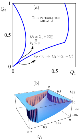
Figure 4: (a) The integration region $\mathcal{A}$ for the integral Eq. (78) to calculate the current due to interactions. The two boundaries for the integration area close to the origin stemming from the signs of $k_{2}$ and $k_{2^{\prime}}$ are indicated. (b) The $\Xi(Q_{1},Q_{3})=\xi(k_{\textrm{F}}Q_{1},k_{\textrm{F}}Q_{3})/\varepsilon_{\textrm{F}}$ function, a dimensionless version of $\xi(q_{1},q_{3})$ Eq. (74), important in the calculation using the method of steepest decent.

To proceed, we consider the low temperature limit $T/T_{\textrm{F}}\ll 1$ by using the method of steepest decent: Due to the exponential function $e^{\frac{T_{\textrm{F}}}{T}\Xi(Q_{1},Q_{3})}$ the maximum of $\Xi(Q_{1},Q_{3})$ will dominate the integral for $T/T_{\textrm{F}}\rightarrow 0$, since $\Xi(Q_{1},Q_{3})\leq 0$. The maxima are $\Xi(0,0)=0$ and $\Xi(0,1)=0$ and $\Xi(Q_{1},Q_{3})$ is shown in Fig. 4(b). For a decreasing interaction the area of $Q_{1}\ll 1$ and $Q_{3}\ll 1$ dominates even though the integrand is zero for $Q_{1}=Q_{3}\rightarrow 0$. Therefore we expand around the maximum $(Q_{1},Q_{3})=(0,0)$ to get the lowest order result in $T/T_{\textrm{F}}$. In view of the integration region Fig. 4(a), we use $Q_{3}=Q_{1}\equiv Q$ in the integral Eq.(78) and thereby do the $Q_{3}$ integral using the approximate limits seen in Fig. 4(a), i.e.

$$\int_{Q_{1}-Q_{1}^{2}}^{Q_{1}+3Q_{1}^{2}}\!\!\!\!\!\!\!1\textrm{d}Q_{3}=4Q_{1}^{2}.$$ (79)

To model the symmetrized potential $\widetilde{V}_{q}$ for small $q$, we include the deviation from a constant as described in Eq. (52). This gives

$$\frac{Q_{1}Q_{3}}{Q_{1}+Q_{3}}|U(Q_{1},Q_{3})|^{2}\bigg{|}_{Q_{3}=Q_{1}\equiv Q}\!\!\!\!\rightarrow V_{0}^{4}\left(\frac{k_{\textrm{F}}}{q_{0}}\right)^{4}\frac{9}{2}Q^{5}$$ (80)

to lowest order in $Q$. In the exponential we keep $\Xi$ to lowest order in $Q$, i.e.

$$e^{\frac{T_{\textrm{F}}}{T}\Xi(Q_{1},Q_{3})}\rightarrow e^{-2Q\frac{T_{\textrm{F}}}{T}}.$$ (81)

So using the lowest order in $Q$ in the integrand (leading to lowest order in $T$) the interacting contribution to the current is:

$$I^{\textrm{int}}= \frac{3(-e)Lm^{3}}{32\pi^{4}\hslash^{7}k_{\textrm{F}}}\ e^{-\frac{T_{\textrm{F}}}{T}}\!\!\!\int_{0}^{\infty}\!\!\!\textrm{d}Q\ V_{0}^{4}\left(\frac{k_{\textrm{F}}}{q_{0}}\right)^{4}\frac{9}{2}Q^{5}$$

$$\times 4Q^{2}e^{-2Q\frac{T_{\textrm{F}}}{T}}\bigg{[}\frac{T_{\textrm{F}}\Delta T}{T^{2}}(0-1)-\frac{eV}{k_{\textrm{B}}T}\bigg{]}$$ (82)

$$\simeq \frac{8505}{2048\pi^{4}}e^{-\frac{T_{\textrm{F}}}{T}}\frac{e}{\hslash}\frac{(V_{0}k_{\textrm{F}})^{4}}{\varepsilon_{\textrm{F}}^{3}}$$

$$\times(Lk_{\textrm{F}})\bigg{(}\frac{k_{\textrm{F}}}{q_{0}}\bigg{)}^{4}\bigg{(}\frac{T}{T_{\textrm{F}}}\bigg{)}^{7}\bigg{[}\frac{\Delta T}{T}+\frac{eV}{\varepsilon_{\textrm{F}}}\bigg{]}$$ (83)

to lowest order in temperature. This is the result stated in the text in Eq. (55).

References

• (1) B. J. van Wees et al., Phys. Rev. Lett. 60, 848 (1988).
• (2) D. A. Wharam et al., J. Phys. C 21, L209 (1988).
• (3) L. I. Glazman, G. B. Lesovik, D. E. Khmelnitskii, and R. I. Shekhter, JETP Lett. 48, 238 (1988).
• (4) A. M. Chang, Rev. Mod. Phys. 75, 1449 (2003).
• (5) M. P. A. Fisher and L. I. Glazman, in Mesoscopic Electron Transport, edited by G. S. L. Kowenhoven and L. Sohn (NATO ASI Series E, Kluwer Ac. Publ., Dordrecht, 1997).
• (6) D. L. Maslov, Lecture notes for the LXXXI Les Houches Summer School (2004), cond-mat/0506035.
• (7) N. A. Mortensen, K. Flensberg, and A.-P. Jauho, Phys. Rev. Lett. 86, 1841 (2001).
• (8) M. Pustilnik, E. G. Mishchenko, L. I. Glazman, and A. V. Andreev, Phys. Rev. Lett. 91, 126805 (2003).
• (9) B. Y.-K. Hu and K. Flensberg, in Hot Carriers in Semicondoctors (HCIS-9), edited by K. H. et al. (Plenum Press, New York, 1996), p. 421.
• (10) This statement is still true for energy bands like $\varepsilon_{k}\propto k^{4}$ or $\varepsilon_{k}\propto k^{2}+ak^{4}$ for $a>0$. A special case is linear dispersion where two-particle collisions can change the distribution. However, even for this case the two-particle collisions cannot change the number of left- and right movers and hence not the current, as shown in Appendix A.
• (11) Bill Sutherland, “Beautiful Models”, World Scientific, 2004, Sections 1.3-1.5
• (12) A related recent work studied a different aspect of three-particle processes, namely their influence on the spectral function of 1D fermions, M. Khodas, M. Pustilnik, A. Kamenev, and L.I. Glazman, cond-mat/0702505.
• (13) A. M. Lunde, K. Flensberg, and L. I. Glazman, Phys. Rev. Lett. 97, 256802 (2006).
• (14) H. van Houten, L. W. Molenkamp, C. W. J. Beenakker, and C. T. Foxon, Semicond. Sci. Technol. 7, B215 (1992).
• (15) Y. V. Sharvin, Zh. Eksp. Teor. Fiz. 48, 984 (1965), [Eng. translation: Sov. Phys. JETP 21, 655 (1965)].
• (16) V. L. Gurevich, V. B. Pevzner, and K. Hess, Phys. Rev. B 51, 5219 (1995).
• (17) H. Akera and T. Ando, Phys. Rev. B 41, 11967 (1990).
• (18) V. L. Gurevich, V. B. Pevzner, and E. W. Fenton, J. Phys.: Condens. Matter 10, 2551 (1998).
• (19) Y. M. Sirenko, V. Mitin, and P. Vasilopoulos, Phys. Rev. B 50, 4631 (1994).
• (20) C.N. Yang, Phys. Rev. 168, 1920 (1968).
• (21) E.H. Lieb and W. Liniger, Phys. Rev. 130, 1605 (1963).
• (22) See e.g., M.A. Cazalilla, Physical Review A 67, 053606 (2003). The interaction potential between Fermions is written there in a slightly different form, which however can be reduced (M. Khodas, A. Kamenev, L.I. Glazman, unpublished) to the one we present in the text.
• (23) We assume that electrons in the channel produce some image charges in a distant gate. As the result, the Coulomb interaction is cut off at some distance $\sim 2\pi/q_{0}$ large compared to the Fermi wavelength.
• (24) Note here that the sign of the conductance correction is negative even though there is a positive sign in Eq.(55). This is due to the way the bias is defined the left contact having the higher chemical potential.
• (25) N. F. Mott and H. Jones, The Theory of the Properties of Metals and Alloys, 1st ed. (Clarendon, Oxford, 1936).
• (26) Surprisingly, Mott formula still yields a reasonably good approximation for thermopower even if the temperature is comparable to the energy scale over which the transmission amplitude changes value, see A. M. Lunde and K. Flensberg, J. Phys.: Condens. Matter 17, 3879 (2005).
• (27) L. W. Molenkamp et al., Phys. Rev. Lett. 65, 1052 (1990).
• (28) L. W. Molenkamp et al., Phys. Rev. Lett. 68, 3765 (1992).
• (29) N. J. Appleyard et al., Phys. Rev. Lett. 81, 3491 (1998).