Virial coefficients and demixing of athermal nonadditive mixtures

Abstract

We compute the fourth virial coefficient of a binary nonadditive hard-sphere mixture over a wide range of deviations from diameter additivity and size ratios. Hinging on this knowledge, we build up a $y$ expansion [B. Barboy and W. N. Gelbart, J. Chem. Phys. 71, 3053 (1979)] in order to trace the fluid-fluid coexistence lines which we then compare with the available Gibbs-ensemble Monte Carlo data and with the estimates obtained through two refined integral-equation theories of the fluid state. We find that in a regime of moderately negative nonadditivity and largely asymmetric diameters, relevant to the modelling of sterically and electrostatically stabilized colloidal mixtures, the fluid-fluid critical point is unstable with respect to crystallization.

I Introduction

A binary mixture of hard spheres is an established prototype model for understanding excluded-volume phenomena relevant to the equilibrium statistical mechanics of some complex fluids bou-nez86 . The model is characterized by the impenetrable diameters of the two species $\sigma_{1}$ and $\sigma_{2}$ and by a cross diameter $\sigma_{12}=(1/2)(\sigma_{1}+\sigma_{2})(1+\Delta)$, where the dimensionless quantity $\Delta$ accounts for deviations of the inter-species repulsive interactions from additivity. As is well known, in a real system the repulsive effects are associated with the overlap between the electron clouds of colliding molecules. However, even in a rare-gas mixture the Lorentz rule ($\Delta=0$) is not systematically satisfied  rowlinson . Deviations from additivity are expected to become more and more pronounced with increasing pressures. In this respect, notwithstanding its crudeness, the hard-sphere model contains some basic features which can be used to sketch, for example, the phase behavior of binary fluids at very high pressures ($\sim 1$ GPa) shout . Deviations from additivity are also manifest in the “effective” interactions which characterize some complex polydisperse fluids such as colloid-polymer mixtures louis .

In general, a bidisperse mixture of hard spheres may exist in a surprisingly rich variety of both ordered and disordered phases whose formation is driven by entropic effects which depend on the diameter ratio $q=\sigma_{2}/\sigma_{1}$ (we conventionally identify the larger particles as species $1$ in such a way that $q\leq 1$), on the deviation from additivity $\Delta$, and on the mole fractions $x_{1}$ and $x_{2}=1-x_{1}$ of the two species, where $x_{1}=N_{1}/(N_{1}+N_{2})$ frenk . For largely asymmetric size ratios ($q<0.3$) and in the absence of nonadditive effects ($\Delta=0$), a mixture tends to phase separate, as a result of osmotic depletion effects, when the larger particles are sufficiently dilute bh1 . However, Monte Carlo (MC) simulations show that in these conditions the demixing transition is preempted by the freezing of the larger particles dre .

The thermodynamic and phase-stability properties of a system turn out to be considerably affected by an even modest degree of nonadditivity. In a nonadditive hard-sphere (NAHS) mixture, the dominant mechanism underlying phase separation is different than in the additive case. First of all, the positive or negative nature of the nonadditivity is critical as to the type of thermodynamic behavior that is exhibited by the mixture. For $\Delta<0$ the model shows a trend towards hetero-coordination and is able to reproduce the large compositional fluctuations that are observed in some liquid and amorphous mixtures albas ; gaz-past1 ; gaz-past2 . On the contrary, for $\Delta>0$ even an equal-sized NAHS mixture exhibits phase separation for high enough densities. This phenomenon is due to the extra repulsion between unlike spheres, which promotes the homo-coordination. The symmetric (equal-diameter) case has been investigated with a variety of theoretical methods tenne ; mazo ; nix ; bpgg ; gazzillo ; lala ; kahl ; sfg ; spg . A number of phenomenological equations of state have been proposed as well ree2 ; hamad1 ; hamad2 . Furthermore, computer simulation studies have been performed for both negative and positive values of the nonadditivity parameter melynk ; adams ; gapa ; amar . Correspondingly, the critical density as well as the universality class which the NAHS model belongs to have been determined yethi ; goz .

So far, the asymmetric case has been studied much less than the symmetric one. The first simulation experiment of a NAHS mixture with similar diameters of the two species was carried out by Rovere and Pastore who traced the phase diagram by means of the Gibbs-ensemble Monte Carlo (GEMC) method rovere . Hamad performed Molecular Dynamics (MD) simulations and calculated the compressibility factor of a NAHS mixture for a number of values of $q$ and $\Delta$ hamad3 . GEMC simulations of a highly asymmetric ($q=0.1$) binary mixture show that fluid-fluid phase separation may occur on account of a rather small amount of nonadditivity dij2 , as had been already conjectured by Biben and Hansen bh2 . A reliable theoretical approach to study the phase diagram of NAHS mixture in a strongly asymmetric regime is based on the calculation of the effective potential between the larger particles. Such an effective potential is obtained upon integrating out the degrees of freedom associated with the smaller spheres lou2 ; re ; lr ; louis1 . Recently, we have shown, by means of integral-equation theories, that a stable fluid-fluid phase separation may occur for moderate size ratios and for a small amount of nonadditivity pellican06 . Another useful theoretical approach is based on the calculation of the residual multiparticle entropy complemented by MC numerical simulations sg . This approach has been applied by Saija and Giaquinta to study the weakly asymmetric case ($q\geq 0.75$).

Some efforts in the direction of studying NAHS mixtures by means of analytical theories have been also made by developing more refined equations of state (EOS) as compared with those obtained via a crude virial expansion. Schaink introduced an EOS whose derivation is reminiscent of the scaled particle theory and is valid in the symmetric as well as in the asymmetric case schaink . More recently, Santos and coworkers proposed an EOS that relies on the exact second and third virial coefficients and requires as an input the compressibility factor of the one-component system santos .

In this paper we evaluate the fourth virial coefficient of a bidisperse NAHS mixture for a number of diameter ratios which span a wide range of accessible values and for $-0.05\leq\Delta\leq 0.5$. As far as we know, the only published virial coefficients beyond the third one are due to Vlasov and Masters vlasov . However, these authors computed the virial coefficients of the mixture up to the sixth order for the size ratio $q=0.1$ only and for just one positive value of the nonadditivity $(\Delta=0.1)$.

Even a reduced number of virial coefficients can be used to construct approximate expansions which turn out to be quite reliable over a wider density range than the original virial expansion bou-nez86 . It is in this conceptual framework that we aim at probing in this paper the reliability of the so-called y expansion, originally proposed by Barboy and Gelbart (BG) barboy1 . We use this approach to calculate the fluid-fluid phase separation lines and compare the results with the available Gibbs-ensemble Monte Carlo data and with the results of some reliable integral-equation closures of the Ornstein-Zernike equations pellican06 .

The paper is organized as follows: In Section II we present the numerical procedure used to calculate the fourth virial coefficient and the explicit expression of the BG EOS for a binary hard-sphere mixture. In Section III we present the phase diagram calculated for a number of size ratios. Some concluding remarks are finally given in Section IV.

II The virial coefficients and the Barboy-Gelbart equation of state

The virial expansion can be written as:

$$\beta P=\rho+B\rho^{2}+C\rho^{3}+D\rho^{4}+\ldots$$ (1)

where P is the pressure, $\beta$ is the inverse temperature in units of the Boltzmann constant, and $\rho=\rho_{1}+\rho_{2}$, $\rho_{i}$ $(i=1,2)$ being the particle number density of the i-th species. In a mixture, at variance with the one-component case, the virial coefficients $B,C,D\ldots$ also depend on the relative concentration of the two species. In particular, the fourth-order coefficient reads:

$$D=D_{1111}x_{1}^{4}+4D_{1112}x_{1}^{3}x_{2}+6D_{1122}x_{1}^{2}x_{2}^{2}+4D_{1222}x_{1}x_{2}^{3}+D_{2222}x_{2}^{4}$$ (2)

In Eq.(2) the coefficients $D_{1111}$ and $D_{2222}$ can be calculated through the corresponding expression for a monodisperse fluid of particles with diameter $\sigma_{1}$ or $\sigma_{2}$, respectively. The cluster integrals $D_{1112}$ and $D_{1122}$ can be represented with the following four-point color graphs:

(3)

(4)

The open and solid circles identify in each graph particles belonging to species 1 and 2, respectively. Each bond contributes a factor to the integrand in the form of a Mayer step function. Space integration is carried out over all the vertices of the graph. We refer the reader for more details on the algorithm to fiumara .

The coefficient $D_{1222}$ is obtained from the general expression of $D_{1112}$ by merely interchanging the larger with the smaller particles and vice-versa. The Monte Carlo results for the composition-independent coefficients $D_{\alpha\beta\gamma\delta}$ (with $\alpha,\beta,\gamma,\delta=1,2$) are given in tables 1-6 over the whole range of $q$ for $\Delta\leq 0.5$. As $q\rightarrow 1$, all the coefficients tend to the value $2.6362...$ (in units of $\sigma_{1}^{9}$) of the one-component fluid. In the opposite limit of $q\rightarrow 0$ the partial coefficient $D_{1112}$ approaches the exact result $1/4(\pi\sigma_{1}^{3}/6)$ fiumara . The knowledge of the fourth virial coefficient allows one to derive the BG expansion up to the fourth order upon expanding the EOS in powers of the variables $y_{i}=\rho_{i}/(1-\eta)$, where $\eta=\pi\rho_{1}\sigma_{1}^{3}/6+\pi\rho_{2}\sigma_{2}^{3}/6$:

$$\beta P=\sum_{\alpha}y_{\alpha}+\sum_{\alpha\beta}A_{\alpha\beta}y_{\alpha}y_{\beta}+\sum_{\alpha\beta\gamma}A_{\alpha\beta\gamma}y_{\alpha}y_{\beta}y_{\gamma}+\sum_{\alpha\beta\gamma\delta}A_{\alpha\beta\gamma\delta}y_{\alpha}y_{\beta}y_{\gamma}y_{\delta}$$ (5)

where the coefficients

$$A_{\alpha\beta}=B_{\alpha\beta}-\frac{\pi}{6}\frac{\sigma_{\alpha}^{3}+\sigma_{\beta}^{3}}{2}$$ (6)

$$A_{\alpha\beta\gamma}=C_{\alpha\beta\gamma}-\frac{\pi}{9}(\sigma_{\gamma}^{3}A_{\alpha\beta}+\sigma_{\alpha}^{3}A_{\gamma\beta}+\sigma_{\beta}^{3}A_{\alpha\gamma})-\frac{\pi^{2}}{108}(\sigma_{\beta}^{3}\sigma_{\gamma}^{3}+\sigma_{\alpha}^{3}\sigma_{\gamma}^{3}+\sigma_{\beta}^{3}\sigma_{\alpha}^{3})$$ (7)

$$A_{\alpha\beta\gamma\delta} = D_{\alpha\beta\gamma\delta}-\frac{\pi}{8}(\sigma_{\delta}^{3}A_{\alpha\beta\gamma}+\sigma_{\alpha}^{3}A_{\delta\beta\gamma}+\sigma_{\beta}^{3}A_{\alpha\delta\gamma}+\sigma_{\gamma}^{3}A_{\alpha\beta\delta})$$ (8)

$$- \frac{\pi^{2}}{72}(\sigma_{\gamma}^{3}\sigma_{\delta}^{3}A_{\alpha\beta}+\sigma_{\beta}^{3}\sigma_{\delta}^{3}A_{\alpha\gamma}+\sigma_{\alpha}^{3}\sigma_{\beta}^{3}A_{\gamma\beta}+\sigma_{\gamma}^{3}\sigma_{\alpha}^{3}A_{\delta\beta}+\sigma_{\gamma}^{3}\sigma_{\beta}^{3}A_{\alpha\delta}+\sigma_{\alpha}^{3}\sigma_{\beta}^{3}A_{\delta\gamma})$$

$$- \frac{\pi^{3}}{864}(\sigma_{\beta}^{3}\sigma_{\gamma}^{3}\sigma_{\delta}^{3}+\sigma_{\alpha}^{3}\sigma_{\gamma}^{3}\sigma_{\delta}^{3}+\sigma_{\beta}^{3}\sigma_{\alpha}^{3}\sigma_{\delta}^{3}+\sigma_{\beta}^{3}\sigma_{\gamma}^{3}\sigma_{\alpha}^{3})$$

are determined so as to ensure the low-density expansion of Eq.(5) to coincide with the fourth-order virial expansion reported in Eq.(1). The quantities $B_{\alpha\beta}$ and $C_{\alpha\beta\gamma}$ are the second and third virial coefficients, respectively, which are available analytically bou-nez86 . In the limit $\Delta\rightarrow 0$, the first three terms of Eq.(5), which correspond to the third order expansion of the BG EOS, reduce to the compressibility equation-of-state of the Percus-Yevick theory. Upon rearranging the above relations, we can write:

$$\beta P=\sum_{i=1}^{\infty}\frac{\rho^{i}A_{i}(x)}{(1-\eta)^{i}}$$ (9)

where

$$A_{1}(x) = 1$$

$$A_{2}(x) = x_{1}^{2}A_{11}+2x_{1}(1-x_{1})A_{12}+(1-x_{1})^{2}A_{22}$$

$$A_{3}(x) = x_{1}^{3}A_{111}+3x_{1}^{2}(1-x_{1})A_{112}+3x(1-x_{1})^{2}A_{122}+(1-x_{1})^{3}A_{222}$$

$$A_{4}(x) = x_{1}^{4}A_{1111}+4x_{1}^{3}(1-x_{1})A_{1112}+6x_{1}^{2}(1-x_{1})^{2}A_{1122}+4x_{1}(1-x_{1})^{3}A_{1222}$$

$$+ (1-x_{1})^{4}A_{2222}$$

As we shall see in the following Section, the inclusion of the fourth virial coefficient definitely improves the performance of the BG EOS over the third-order one. A more convincing test of the reliability of the BG EOS including the fourth virial coefficient is provided by the comparison of the predictions for the fluid-fluid phase separation threshold with the numerical simulation data. In order to trace the phase-coexistence curve, we need the Gibbs free energy. We start by calculating the Helmholtz free energy:

$$\frac{{\beta}A}{N} = \int_{0}^{\rho}\Big{(}\frac{Z}{\rho}\Big{)}d{\rho}{}$$ (10)

$$= {}[\ln\big{(}{\rho}{\Lambda}^{3}\big{)}-1]+\sum_{k=1}^{2}x_{k}\ln(x_{k})-\ln(1-\eta)+\sum_{k=1}^{\infty}\frac{\rho^{i}A_{i+1}(x)}{i(1-\eta)^{i}}$$

where $Z=\beta P/\rho$ is the compressibility factor; the Gibbs free energy then follows as hansen ; bijor :

$$\frac{\beta G}{N}=\frac{\beta A}{N}+Z.$$ (11)

The fluid-fluid coexistence curves are obtained through the common-tangent construction of the Gibbs free energy at constant pressure.

III Results and Discussion

We present in Figs. 1 and 2 the compressibility factor calculated for different values of the size ratio and of the nonadditivity parameter. The fourth-order BG expansion (BG4) of the EOS is in better agreement with the simulation data provided by Hamad hamad3 than the corresponding third-order expansion (BG3), expecially for large packing fractions. However, as shown in Fig. 2, this improvement is not systematic.

III.1 Species with not too dissimilar sizes

We compare in Fig. 3 our results for the phase coexistence thresholds with those obtained by Rovere and Pastore for $q=0.8333$ and $\Delta=0.182$ in their GEMC simulations rovere . Unfortunately, we could not report in the figure the simulation critical parameters explicitly because the coexistence curve becomes rather flat around there and a reasonable determination of them would typically require very long computations rovere . As shown in the top panel of Fig. 3, both BG estimates of the EOS appear to underestimate the critical pressure, which is located at the minimum of the phase coexistence curve, by about $20\%$. However, on account of the large fluctuations that affect the system on approaching the critical point, it may be possible that the pressure measured inside the two simulation boxes is not sufficiently stable against the value imposed from outside. This fact might be partially responsible for the discrepancy observed between the GEMC data and the BG estimates. The growth of fluctuations near the critical point is apparent in the bottom panel of Fig. 3 where we report the error bars associated with the GEMC results for the coexistence densities plotted as a function of the relative composition. In fact, in the density-concentration plane, the present theoretical predictions fall inside the simulation error bars around the critical point. Overall, the BG4 critical pressure and density show a better agreement with the GEMC simulation results as compared with their BG3 counterparts.

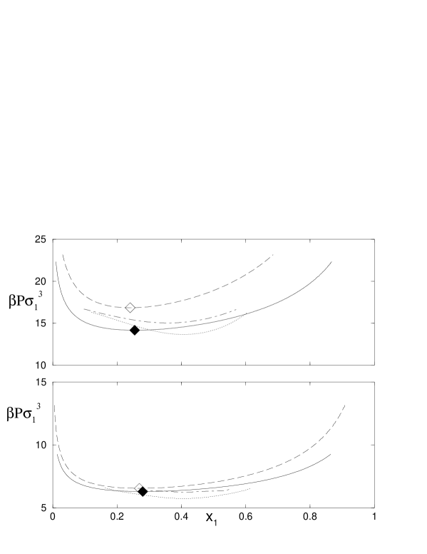
Figure 6: Fluid-fluid coexistence in the pressure-composition plane for $q=0.6$: top panel, $\Delta=0.05$; bottom panel, $\Delta=0.1$. The continuous and dashed curves represent the BG4 and BG3 binodal lines, respectively. The critical point is identified with solid (BG4) and open (BG3) diamonds. The dotted and dot-dashed lines represent the RY and MHNC predictions, respectively pellican06 ..

We also show the behavior of the analytical EOS for size ratios $q=0.75$ (Fig. 4) and $q=0.6$ (Fig. 5) and for two values of the nonadditivity parameter $\Delta=0.05,0.1$ which are particularly meaningful for Helium-Xenon mixtures at high pressure pellican06 . In this case the critical point falls at medium-high packing fractions and we found no simulation data in the literature to compare with. Hence, we compare the BG3 and BG4 estimates of the phase separation curves with the predictions of two integral-equation theories pellican07 , i.e., the modified hypernetted-chain (MHNC) mhnc and the Rogers-Young (RY) ry closures of the Ornstein-Zernike equations. In these approximate theories two internal parameters are adjusted so as to ensure the equality of the two osmotic compressibilities that are respectively obtained via number fluctuations or upon differentiating the virial pressure pellican06 . We show in Fig. 4 (upper panel) the binodal line for $q=0.75$ and $\Delta=0.05$. The current numerical estimates for the critical mole fraction and for the reduced pressure are reported in Table LABEL:t7. It is evident that the BG4 critical pressure is in better agreement with the corresponding integral-equation estimates. The differences between the BG3 and BG4 expansions are smaller for $\Delta=0.1$ (see Fig. 4, bottom panel). Even in this case, the BG4 critical parameters are in better agreement with the corresponding MHNC and RY estimates. As for the shape of these curves, we note that the values of the constant-pressure Gibbs free energy obtained from integral-equation theories was fitted through a fourth-order polynomial curve (see Fig. 6, upper panel) pellican06 . Overall, the resulting agreement with the current results for the Gibbs free energy is good. However, the implementation of the Maxwell construction requires the concentration derivative of the Gibbs free energy (see Fig. 6). The discrepancies observed in the shapes of the phase-separation curves obtained with the two methods discussed above (EOS expansions and integral-equation theories) may be likely due to the estimate of this latter quantity. In fact, we suspect that the derivative of the polynomial curve used to fit the integral-equation data for the Gibbs free energy probably is not flexible enough as one is lead to argue after observing the shapes of the corresponding BG3 and BG4 curves.

The BG4 fluid-fluid critical point is in better agreement with the corresponding integral-equation estimate also for $q=0.6$ (see Fig. 5). In fact, for $\Delta=0.05$ the BG4 critical pressure, that is reported in Table LABEL:t8, falls in between the MHNC and RY values as for $q=0.6$ (see Table LABEL:t7). As far as the critical concentration is concerned, in passing from $q=0.75$ to $q=0.6$, the BG4 estimate moves to lower $x_{1}$ values in a more distinct way than its MHNC and RY courterparts. Finally, for larger values of the nonadditivity parameter ($\Delta=0.1$), the differences in the critical parameters estimated with these approaches smooth over, as previously shown for $q=0.75$ (see Table LABEL:t8).

III.2 Highly asymmetric regime

We start commenting the results obtained for $q=0.1$ and nonadditivity $\Delta=0.2,0.3,0.4,0.5$. We compare in Fig. 7 the fluid-fluid coexistence curves obtained by means of the BG3 and BG4 estiamtes of the EOS with the GEMC simulations reported in dij2 . As already observed for larger size ratios, the BG4 curve shows a better agreement with the simulation data in the region around the critical point, and this improvement is more evident for low values of the nonadditivity parameter. On the other side, for larger values of $\Delta$, the BG3 and BG4 estimates become very close to each other, as was also the case of mixtures with not too dissimilar species. This effect is probably related to the comparatively lower packing fractions of the demixing region that is observed for larger nonadditivities. In fact, the mixture is less correlated at low densities and one may then expect that the differences between the fourth and the third-order estimates of the EOS tend to disappear. Figure 8 shows the critical pressure and packing fraction plotted as a function of the nonadditivity parameter. We also observed a crossover in the BG4 critical pressure versus its BG3 value upon further decreasing $\Delta$: viz., the BG4 values get lower than the BG3 ones. This observation is particularly significant because the BG3 critical pressure tends to diverge in the limit of additive mixtures ($\Delta=0$), whilst the BG4 value apparently remains finite.

As pointed out by many authors, the regime of low or even negative values of the nonadditivity parameter is interesting for the application of the model to sterically and electrostatically stabilized colloidal mixtures. In particular, Louis and coworkers used the Alexander-de Gennes theory with the Derjaguin approximation in order to estimate the value of the nonadditivity parameter for a polymethylmetrylacrilate mixture stabilized by a poly-12-hydroxysteric acid brush lou2 . They obtained $\Delta=-0.01$ for $q=0.1075$. We present in the bottom panel of Fig. 9 the BG4 fluid-fluid binodal line with its critical point for a mixture with size ratio $q=0.1$ and compare it with the fluid-solid binodal line as reported in lou2 . For negative values of $\Delta$, the demixing transition should be preempted by the formation of the solid phase because a stable demixing is expected to occur in very asymmetric mixtures only louis1 ; santos1 . In ref. lou2 , the adopted crystal structure in order to evaluate the fluid-solid binodal, is an FCC lattice of large spheres (permeated by a fluid of small spheres). Actually, we find that demixing occurs for very high values of the larger-particles packing fraction (see the inset of Fig. 9) and for very low values of the smaller-particles packing fraction. The corresponding BG4 critical point, with coordinates $\eta_{1}=0.67$ and $\eta_{2}=0.0014$, falls well inside the region of stability of the solid phase. Louis and coworkers also estimated that for positive values of the nonadditivity parameter the critical point remains metastable up to $\Delta\approx 0.2$ lou2 . In agreement with their prediction, for $\Delta=0.25$ the fluid-fluid critical point, located by both the BG3 and BG4 expansions, falls below the freezing line (see the top panel of Fig. 9).

IV Concluding remarks

In this paper we discussed the fourth virial coefficient of binary hard-sphere mixtures, which has been computed for different values of the nonadditivity parameter and of the size ratio. We have shown that its use within the $y$ expansion originally proposed by Barboy and Gelbart improves over the description of the fluid-fluid phase separation provided by the same expansion truncated at the third order, the more so for small values of the size ratio and of the nonadditivity parameter. In particular, we found that the pressure calculated at the critical point through the fourth-order expansion does not diverge in the limit of small values of the nonadditivity parameter and of largely asymmetric size ratios. This feature allowed us to predict that, within this approximation, the critical point is unstable with respect to crystallization in the regime relevant to colloidal mixtures.

Table 1: Fourth-order partial virial coefficients as a function of the size ratio for $\Delta=0.05$. The numerical values are given in units of $\sigma_{1}^{9}$. The error on the last significant figure is enclosed in parentheses.

$q$	$D_{1112}$	$D_{1122}$	$D_{1222}$
0.05	0.0835(3)	5.53(1)$\cdot 10^{-5}$	2.064(1)$\cdot 10^{-8}$
0.10	0.1201(4)	5.271(9)$\cdot 10^{-4}$	1.3981(6)$\cdot 10^{-6}$
0.15	0.1661(5)	2.073(4)$\cdot 10^{-3}$	1.6840(8)$\cdot 10^{-5}$
0.20	0.2225(6)	5.67(1)$\cdot 10^{-3}$	9.988(6)$\cdot 10^{-5}$
0.25	0.2900(7)	1.267(2)$\cdot 10^{-2}$	4.019(2)$\cdot 10^{-4}$
0.30	0.3697(8)	2.485(4)$\cdot 10^{-2}$	1.2645(8)$\cdot 10^{-3}$
0.40	0.569(1)	7.46(1)$\cdot 10^{-2}$	7.857(6)$\cdot 10^{-3}$
0.50	0.828(1)	0.1806(4)	3.303(3)$\cdot 10^{-2}$
0.60	1.153(2)	0.3807(8)	0.1084(1)
0.70	1.554(2)	0.728(1)	0.2990(3)
0.75	1.784(2)	0.977(1)	0.4726(3)
0.80	2.036(3)	1.292(2)	0.7269(8)
0.85	2.309(2)	1.683(2)	1.0914(9)
0.90	2.606(3)	2.166(4)	1.604(2)
0.95	2.927(4)	2.755(6)	2.311(3)

Table 2: Fourth-order partial virial coefficients as a function of the size ratio for $\Delta=0.1$ (see also the caption of Table I).

$q$	$D_{1112}$	$D_{1122}$	$D_{1222}$
0.05	0.1201(4)	5.37(1)$\cdot 10^{-5}$	2.3824(8)$\cdot 10^{-8}$
0.10	0.1686(7)	6.15(2)$\cdot 10^{-4}$	1.620(1)$\cdot 10^{-6}$
0.15	0.2284(6)	2.505(4)$\cdot 10^{-3}$	1.959(1)$\cdot 10^{-5}$
0.20	0.3007(7)	6.94(1)$\cdot 10^{-3}$	1.1664(6)$\cdot 10^{-4}$
0.25	0.3863(8)	1.560(2)$\cdot 10^{-2}$	4.710(3)$\cdot 10^{-4}$
0.30	0.4865(9	3.073(6)$\cdot 10^{-2}$	1.486(1)$\cdot 10^{-3}$
0.40	0.735(1)	9.26(2)$\cdot 10^{-2}$	9.298(7)$\cdot 10^{-3}$
0.50	1.053(2)	0.2249(4)	3.934(3)$\cdot 10^{-2}$
0.60	1.451(2)	0.4750(8)	0.1298(1)
0.70	1.938(3)	0.909(2)	0.3602(3)
0.75	2.216(2)	1.220(2)	0.5710(4)
0.80	2.519(3)	1.613(3)	0.8810(9)
0.85	2.849(2)	2.103(2)	1.326(1)
0.90	3.206(4)	2.704(5)	1.953(2)
0.95	3.591(4)	3.442(6)	2.822(3)

Table 3: Fourth-order partial virial coefficients as a function of the size ratio for $\Delta=0.2$ (see also the caption of Table I).

$q$	$D_{1112}$	$D_{1122}$	$D_{1222}$
0.05	0.2226(6)	-2.277(2)$\cdot 10^{-4}$	3.116(1)$\cdot 10^{-8}$
0.10	0.3007(7)	1.15(2)$\cdot 10^{-4}$	2.134(1)$\cdot 10^{-6}$
0.15	0.3945(8)	2.022(6)$\cdot 10^{-3}$	2.595(1)$\cdot 10^{-5}$
0.20	0.506(1)	7.10(2)$\cdot 10^{-3}$	1.5554(8)$\cdot 10^{-4}$
0.25	0.637(1)	1.758(4)$\cdot 10^{-2}$	6.320(4)$\cdot 10^{-4}$
0.30	0.787(1)	3.647(7)$\cdot 10^{-2}$	2.006(1)$\cdot 10^{-3}$
0.40	1.154(2)	0.1150(2)	1.2694(9)$\cdot 10^{-2}$
0.50	1.617(2)	0.2879(5)	5.429(4)$\cdot 10^{-2}$
0.60	2.190(3)	0.616(1)	0.1809(2)
0.70	2.881(4)	1.188(2)	0.5068(5)
0.75	3.274(3)	1.600(2)	0.8071(5)
0.80	3.702(4)	2.118(4)	1.250(1)
0.85	4.166(3)	2.765(4)	1.890(1)
0.90	4.664(5)	3.562(6)	2.795(3)
0.95	5.204(6)	4.528(8)	4.056(4)

Table 4: Fourth-order partial virial coefficients as a function of the size ratio for $\Delta=0.3$ (see also the caption of Table I).

$q$	$D_{1112}$	$D_{1122}$	$D_{1222}$
0.05	0.3697(8)	-2.0687(2)$\cdot 10^{-4}$	3.984(1)$\cdot 10^{-8}$
0.10	0.4865(9)	-3.736(3)$\cdot 10^{-3}$	2.744(1)$\cdot 10^{-6}$
0.15	0.625(1)	-4.857(7)$\cdot 10^{-3}$	3.357(1)$\cdot 10^{-5}$
0.20	0.787(1)	-3.90(2)$\cdot 10^{-3}$	2.022(1)$\cdot 10^{-4}$
0.25	0.974(2)	1.21(5)$\cdot 10^{-3}$	8.261(5)$\cdot 10^{-4}$
0.30	1.188(2)	1.339(9)$\cdot 10^{-2}$	2.635(2)$\cdot 10^{-3}$
0.40	1.705(2)	7.46(3)$\cdot 10^{-2}$	1.683(1)$\cdot 10^{-2}$
0.50	2.350(3)	0.0.2219(7)	7.259(5)$\cdot 10^{-2}$
0.60	3.139(4)	0.514(2)	0.2439(2)
0.70	4.085(5)	1.034(3)	0.6886(6)
0.75	4.622(4)	1.410(2)	1.1001(7)
0.80	5.203(6)	1.188(5)	1.711(2)
0.85	5.833(4)	2.477(4)	2.594(2)
0.90	6.506(7)	3.204(9)	3.849(4)
0.95	7.233(7)	4.09(1)	5.602(5)

Table 5: Fourth-order partial virial coefficients as a function of the size ratio for $\Delta=0.4$ (see also the caption of Table I).

$q$	$D_{1112}$	$D_{1122}$	$D_{1222}$
0.05	0.569(1)	-9.0438(3)$\cdot 10^{-3}$	5.004(1)$\cdot 10^{-8}$
0.10	0.734(1)	-1.7721(2)$\cdot 10^{-2}$	3.462(2)$\cdot 10^{-6}$
0.15	0.929(1)	-3.002(7)$\cdot 10^{-2}$	4.256(4)$\cdot 10^{-5}$
0.20	1.153(2)	-4.597(3)$\cdot 10^{-2}$	2.575(1)$\cdot 10^{-4}$
0.25	1.412(2)	-6.544(6)$\cdot 10^{-2}$	1.0564(6)$\cdot 10^{-3}$
0.30	1.705(2)	-8.75(1)$\cdot 10^{-2}$	3.383(2)$\cdot 10^{-3}$
0.40	2.406(3)	-0.1377(4)	2.178(1)$\cdot 10^{-2}$
0.50	3.274(4)	-0.1898(9)	9.461(7)$\cdot 10^{-2}$
0.60	4.327(5)	-0.236(2)	0.3199(2)
0.70	5.584(6)	-0.280(4)	0.9088(7)
0.75	6.295(5)	-0.299(3)	1.4564(9)
0.80	7.062(7)	-0.314(6)	2.270(2)
0.85	7.890(6)	-0.346(6)	3.452(2)
0.90	8.782(9)	-0.39(1)	5.137(5)
0.95	9.729(9)	-0.46(1)	7.498(7)

Table 6: Fourth-order partial virial coefficients as a function of the size ratio for $\Delta=0.5$. See also caption of table I.

$q$	$D_{1112}$	$D_{1122}$	$D_{1222}$
0.05	0.828(1)	-2.91908(3)$\cdot 10^{-2}$	6.180(1)$\cdot 10^{-8}$
0.10	1.053(2)	-5.6318(3)$\cdot 10^{-3}$	4.295(2)$\cdot 10^{-6}$
0.15	1.316(2)	-9.806(1)$\cdot 10^{-2}$	5.303(4)$\cdot 10^{-5}$
0.20	1.617(2)	-0.15883(3)	3.220(2)$\cdot 10^{-4}$
0.25	1.962(3)	-0.24429(7)	1.3258(7)$\cdot 10^{-3}$
0.30	2.350(3)	-0.3605(1)	4.263(2)$\cdot 10^{-3}$
0.40	3.275(4)	-0.7246(5)	2.761(2)$\cdot 10^{-2}$
0.50	4.410(5)	-1.346(1)	0.12067(8)
0.60	5.781(6)	-2.378(2)	0.4103(3)
0.70	7.409(7)	-4.064(4)	1.1717(9)
0.75	8.326(6)	-5.245(4)	1.882(1)
0.80	10.314(9)	-6.718(7)	2.941(2)
0.85	10.379(7)	-8.578(7)	4.482(3)
0.90	11.52(1)	-10.88(1)	6.686(6)
0.95	12.74(1)	-13.73(2)	9.777(8)

Table 7: Critical molar fractions and reduced pressures for $q=0.75$.

$\Delta$			$x_{1}$	$\beta P\sigma_{1}^{3}$
0.05	BG3		0.34	12.21
	BG4		0.36	10.34
	MHNC		0.44	9.72
	RY		0.43	10.5
0.1	BG3		0.36	4.73
	BG4		0.37	4.54
	MHNC		0.455	4.1
	RY		0.45	4.12

Table 8: Critical molar fractions and reduced pressures for $q=0.60$.

$\Delta$			$x_{1}$	$\beta P\sigma_{1}^{3}$
0.05	BG3		0.241	16.85
	BG4		0.255	14.15
	MHNC		0.405	13.7
	RY		0.36	15.05
0.1	BG3		0.27	6.55
	BG4		0.28	6.30
	MHNC		0.41	5.74
	RY		0.41	6.25

Figure 1: Compressibility factor plotted as a function of the total packing fraction for $q=1/3$, $x_{1}=0.5$: left panel, $\Delta=-0.05$; right panel, $\Delta=0.05$. The continuous and dashed lines represent the BG4 and BG3 estimates, respectively. The solid circles are the MD results by hamad3 . The corresponding fourth-order partial virial coefficients calculated for $\Delta=-0.05$ are: D1112=$0.2304(6)$, D1122=$2.037(5)\cdot 10^{-2}$, D1222=$1.719(1)\cdot 10^{-3}$.

Figure 2: Compressibility factor plotted as a function of the mole fraction for $\Delta=0.2$: left panel, $q=0.25$; right panel, $q=0.5$. Stars: BG4; triangles: BG3; circles: MD results hamad3 .

Figure 3: Fluid-fluid coexistence in the pressure-composition plane (top panel) and density-composition plane (bottom panel) plotted for $q=0.8333$ and $\Delta=0.182$. The continuous and dashed curves represent the BG4 and BG3 binodal lines, respectively. The critical point is identified with solid (BG4) and open (BG3) diamonds. Open circles, with the corresponding error bars in the density-composition plane, represent the GEMC simulation data rovere . The corresponding fourth-order partial virial coefficients are: D1112=$3.752(5)$, D1122=$2.457(3)$, D1222=$1.459(1)$.

Figure 4: Fluid-fluid coexistence in the pressure-composition plane for $q=0.75$: top panel, $\Delta=0.05$; bottom panel, $\Delta=0.1$. The continuous and dashed curves represent the BG4 and BG3 binodal lines, respectively. The critical point is identified with solid (BG4) and open (BG3) diamonds. The dotted and dot-dashed lines represent the RY and MHNC predictions, respectively pellican06 .

Figure 5: Total Gibbs free energy (top panel) and its first derivative (bottom panel) plotted as a function of the mole fraction for $q=0.75$, $\Delta=0.05$ and $\beta P\sigma_{1}^{3}=11.38$. Dashed line: BG3; continuous line: BG4; solid circles: RY closure; dot-dashed line: fourth-order polynomial fit of the RY data.

Figure 7: Fluid-fluid coexistence in the pressure-composition plane for $q=0.1$. The continuous and dashed curves are the BG4 and BG3 binodal lines, respectively. The critical point is identified with solid (BG4) and open (BG3) diamonds. The open symbols represent the GEMC simulation data dij2 obtained for $\Delta=0.5$ (circles), $0.4$ (squares), $0.3$ (diamonds), $0.2$ (triangles).

Figure 8: Reduced pressure (top panel) and total packing fraction (bottom panel), calculated at the critical point for a nonadditive hard-sphere mixture with size ratio $q=0.1$, plotted as a function of the nonadditivity parameter $\Delta$: open diamonds, BG3; solid diamonds, BG4; stars, simulation data dij2 .

Figure 9: Phase diagram calculated for $q=0.2$ and $\Delta=0.25$ (top panel) and for $q=0.1075$ and $\Delta=-0.01$ (bottom panel). Dot-dashed curves: fluid-solid binodal line from lou2 ; the continuous and dashed curves represent the BG4 and BG3 binodal lines, respectively. The critical point is identified with solid (BG4) and open (BG3) diamonds. The continuous lines plotted in the inset represents the BG4 fluid-fluid binodal line. The orresponding fourth-order partial virial coefficients are: D1112=$7.98(1)\cdot 10^{-2}$, D1122=$4.840(4)\cdot 10^{-4}$, D1222=$1.8029(7)\cdot 10^{-6}$.

.

References

- (1) Boublík, T.; Nezbeda, I. Collect. Czech. Chem. Commun. 1986, 51, 2301.
- (2) Rowlinson, J. S. Liquids and liquid mixtures (Butterworth, London, 1969).
- (3) Shouten, J. A. Int J. of Thermophys. 2001, 22, 23.
- (4) Louis, A. A. Philos. T. Roy. Soc. A 2001, 359, 939.
- (5) Frenkel, D. J. Phys.: Condens. Matter 1994, 6, A71-A78.
- (6) Biben, T.; Hansen, J. P. Phys. Rev. Lett. 1991, 66, 2215.
- (7) Dijkstra, M.; van Roij, R.; Evans, R. Phys. Rev. Lett. 1998, 81, 2268; ibid. 1999, 82, 117; Phys. Rev. E 1999, 59, 5744.
- (8) Albas, P.; van der Marel, C.; Geertsman, W.; Meijer, J. A.; van Osten, A. B.; Dijkstra, J.; Stein, P. C.; van der Lugt, W. J. non-crystalline Solids 1984, 61/62, 201.
- (9) Gazzillo, D.; Pastore, G.; Enzo, S. J. Phys.: Condens. Matter 1989, 1, 3469.
- (10) Gazzillo, D.; Pastore, G.; Frattini, R. J. Phys.: Condens. Matter 1990, 2, 8463.
- (11) Tenne, R.; Bergmann, E. Phys. Rev. A 1978, 17, 2036.
- (12) Mazo, R.; Bearman, R. J. J. Chem. Phys. 1990, 93, 6694.
- (13) Nixon, J. H.; Silbet, M. Molec. Phys. 1984, 52, 207.
- (14) Ballone, P.; Pastore, G.; Galli, G.; Gazzillo, D. Molec. Phys. 1986, 59, 275.
- (15) Gazzillo, D. J. Chem. Phys. 1991, 95, 4565.
- (16) Lomba, E.; Alvarez, M.; Lee, L. L.; Almarza, N. E. J. Chem. Phys. 1996, 104, 4180.
- (17) Kahl, G.; Bildstein, B.; Rosenfeld, Y. Phys. Rev. E 1996, 54, 5391.
- (18) Saija, F.; Fiumara, G.; Giaquinta, P. V. J. Chem. Phys. 1998, 108, 9098.
- (19) Saija, F.; Pastore, G.; Giaquinta, P. V. J. Phys. Chem. B 1998, 102, 10368.
- (20) Jung, J.; Jhon, M. S.; Ree, F. H. J. Chem. Phys. 1995, 102, 1349.
- (21) Hamad, E. Z. J. Chem. Phys. 1996, 105, 3222.
- (22) Hammawa, H.; Hamad, E. Z. J. Chem. Soc., Faraday Trans. 1996, 92, 4943.
- (23) Melnyk, T. W.; Sawford, B. L. Molec. Phys. 1975, 29, 891.
- (24) Adams, D. J.; McDonald, I. R. J. Chem. Phys. 1975, 63, 1900.
- (25) Gazzillo D.; Pastore G. Chem. Phys. Lett. (1989) 159, 388.
- (26) Amar, J. G.; Molec. Phys. 1989, 67, 739.
- (27) Jagannathan, K; Yethiraj, A. J. Chem. Phys. 2003, 118, 7907.
- (28) Gǿzdz, W. T. J. Chem. Phys. 119, (2003), 3309.
- (29) Rovere, M.; Pastore, G. J. Phys.: Condens. Matter 1994, 6, A163.
- (30) Hamad, E. Z. Molec. Phys. 1997, 91, 371.
- (31) Dijkstra, M. Phys. Rev. E 1998, 58, 7523.
- (32) Biben, T.; Hansen, J.-P. Physica A 1997, 235, 142.
- (33) Louis, A. A.; Finken, R.; Hansen, J.-P. Phys. Rev. E 2000, 61, R1028.
- (34) Roth, R.; Evans, R. Europhys. Lett. 2001, 53, 271.
- (35) Louis, A. A.; Roth, R., J. Phys.: Condens. Matter 2001, 13, L777.
- (36) Roth, R.; Evans, R.; Louis, A. A., Phys. Rev. E 2001, 64, 051202.
- (37) Pellicane, G.; Saija, F.; Caccamo, C.; Giaquinta, P. V. J. Phys. Chem. B 2006, 110, 4359.
- (38) Saija, F.; Giaquinta, P. V. J. Phys. Chem. B 2002, 106, 2035.
- (39) Schaink, H. M. Z. Naturforsch., A: Phys. Sci. 1993, 48, 899.
- (40) Santos, A.; Lopez de Haro, M.; Yuste, S. B. J. Chem. Phys. 2005, 122, 024514.
- (41) Vlasov, A. Y.; Masters, A. J. Fluid Phase Equilib. 2003, 212, 183.
- (42) Barboy, B.; Gelbart, W. N. J. Chem. Phys. 1979, 71, 3053; J. Stat. Phys. 1980, 22, 709.
- (43) Saija, F.; Fiumara, G.; Giaquinta, P. V. Molec. Phys. 1996, 87, 991.
- (44) Hansen, J. -P., McDonald, I. R. Theory of simple liquids (Academic Press, London, 1986).
- (45) Bjorling, M.; Pellicane, G.; Caccamo, C. J. Chem. Phys. 1999, 111, 6884.
- (46) Pellicane, G.; Saija, F.; Caccamo, C.; Giaquinta, P. V. unpublished.
- (47) Rosenfeld, Y.; Aschroft, N. Phys. Rev. A 1979, 20, 1208.
- (48) Rogers, F.; Young, D. A. Phys. Rev. A 1984, 30, 999.
- (49) A. Santos, A.; Lopez de Haro, M. Phys. Rev. E 2005 72, 010501(R).