Wigner crystal and bubble phases in graphene in quantum Hall regime
Abstract
Graphene, a single free-standing sheet of graphite with honeycomb lattice structure, is a semimetal with carriers that have linear dispersion. A consequence of this dispersion is the absence of Wigner crystallization in graphene, since the kinetic and potential energies both scale identically with density of carriers. We study the ground state of graphene in the presence of strong magnetic field focusing on states with broken translational symmetry. Our mean-field calculations show that at integer fillings a uniform state is preferred whereas at non-integer fillings, Wigner crystal states (with broken translational symmetry) have lower energy. We obtain the phase diagram of the system. We find that it is qualitatively similar to that of quantum Hall systems in semiconductor heterostructures. Our analysis predicts that non-uniform states, including Wigner crystal state, will occur in graphene in the presence of a magnetic field and will lead to anisotropic transport in high Landau levels.
pacs:
73.20.Qt, 73.43.-fI Introduction
Two dimensional electron gas (2DEG), realized either in semiconductor heterostructures or by sprinkling electrons on Helium surface, has been extensively studied over the past few decades. It is known that such a system undergoes phase transition from a uniform state to a state with spontaneously broken translational symmetry, a Wigner crystal, when the carrier density is sufficiently low Wigner (1934) or the temperature is sufficiently high. Grimes and Adams (1979) In case of a 2DEG in semiconductors, this state occurs when the gain from lowering the potential energy by localization outweighs the kinetic energy cost associated with the localization provided that the dispersion of carriers is well-described by an effective mass , . This transition has been theoretically investigated, Wigner (1989) although unequivocal experimental evidence is still lacking. The spectrum of the electron gas changes radically in the presence of a strong magnetic field. The kinetic energy is quantized and each Landau level (the manifold of eigenstates with a given energy) has a macroscopic degeneracy. Since the kinetic energy is fixed for a given Landau level, it is possible to vary the ratio of potential energy and kinetic energy by changing the filling factor within a given Landau level, and the system undergoes a transition from a uniform state to states with broken translational symmetry. Indeed, this transition has been extensively studied theoretically. Das There is strong experimental evidence that the ground state of such a system at filling factors is a Wigner crystal Willett et al. (1988) and that at partial filling factors in high Landau levels, the ground state is non-uniform. Lilly et al. (1999) We remind the Reader that this evidence is obtained from transport measurements and that a direct measurement of spatial density modulation - crystalline structure - is exceedingly difficult since the 2DEG is buried under a substrate.
In this paper, we focus on how these results change when the carries in the 2D gas have a linear dispersion instead of the the usual effective-mass quadratic dispersion. Graphene, a single sheet of graphite with honeycomb lattice structure, is a realization of a system with such carriers. It has the added advantage that such a 2D gas of carriers is not buried under a substrate and is, therefore, amenable to local probes that can investigate the crystalline structure. Graphene is a semimetal in which the valance and conduction bands touch at two inequivalent points and (and four other points related by symmetry). In the vicinity of these points (valleys), the band structure of carriers is well described by where eVÅ is the characteristic velocity and is measured from one of the six points at which the conduction and valance bands touch. Wallace (1947); Nov Due to the linear dispersion of carriers in graphene, potential and kinetic energies both scale as with the carrier density . Therefore, graphene does not undergo Wigner crystallization in the absence of an external magnetic field. Dahal et al. (2006)
In the presence of a magnetic field, however, the kinetic energy is quantized and its ratio with the potential energy can be varied by changing the filling factor. This raises the prospect of Wigner crystal states in graphene. Here, we present a systematic mean-field analysis of the ground state of graphene in the quantum Hall regime, focusing on partial filling of the first few Landau levels. The plan for the paper is as follows. In the next section, we set up the low-energy Hamiltonian for graphene in the presence of magnetic field and recall results for the single-particle spectrum. In Sec. III, we set up the formalism for Hartree-Fock (HF) approximation and discuss its details. In Sec. IV, we present the numerical results we obtain. We discuss the phase diagram of graphene as a function of the partial filling factor and the density profiles. We find that the results closely follow those of non-uniform states in the conventional 2DEG. We end the paper with a brief discussion and conclusions in section V.
II Graphene in Magnetic Field
The low-energy Hamiltonian for electrons in the valley is given by Semenoff (1984); Haldane (1988)
| (1) |
where and are Pauli matrices in the space consisting of two lattice sites and within a single unit cell (The Hamiltonian for the other valley is obtained by complex conjugation). The Hamiltonian in the presence of an magnetic field is obtained by Peirels substitution . In a uniform magnetic field , generated by a vector potential , the Hamiltonian (1) becomes
| (2) |
where is the lowering operator, is the magnetic length, and . The eigenvalues of this Hamiltonian are given by and the corresponding eigenfunctions are given by
| (3) |
for and
| (4) |
for . Here, are the simple harmonic oscillator eigenfunctions defined by and is the sample length in -direction. (In the following, we will use units such that ). Thus, eigenfunctions in graphene are identical to states in a conventional 2DEG, whereas for , the eigenfunctions of graphene are an admixture of wavefunctions on the and lattice sites. Peres et al. (2005) Therefore, we expect that graphene, like conventional 2DEG at partial filling factors, will support non-uniform (Wigner crystal) states.
In the following, we denote crystals with one electron per unit cell, as Wigner crystals, and those with per unit cell as bubble crystals. Koulakov et al. (1996); Goerbig et al. (2004) We also consider modulated stripe states that can be described by oblique, rectangular, or centered rectangular lattices. Côté and Fertig (2000); Ettouhami et al. (2006) We call these states anisotropic Wigner crystals, and the ones having a triangular or square lattice structure as isotropic Wigner crystals.
III Hartree-Fock Hamiltonian
The microscopic Hamiltonian for carriers in graphene consists of the kinetic energy and Coulomb repulsion. We use a pseudospin notation to denote the valley index: corresponds to the valley and corresponds to the valley. In the single-particle basis (3,4) the Hamiltonian is
| (5) |
where is the number of flux quanta in the area of the sample, is the chemical potential, is the Coulomb interaction and is the dielectric constant of graphene (), is the density matrix element defined as
| (6) |
with () the creation (annihilation) operator of the electrons, is the form factor
| (7) |
where is the heavyside function and returns the sign of its argument. This form factor is a linear combination of form factors for wave functions on the two inequivalent lattice sites,
| (8) |
and . Here is the generalized Laguerre polynomial. To obtain the Hamiltonian (5), we have ignored the interaction terms that scatter electrons from one valley to another and are exponentially and algebraically small in where is the lattice constant of graphene ( 5 Å, 100 Å). Goerbig et al. (2006)
The derivation of the HF Hamiltonian from Eq. (5) is straightforward and has been discussed extensively in the literature. Cot ; Côté et al. (1992); Chen and Quinn (1992) When inter-Landau level transitions are ignored, the Hartree-Fock Hamiltonian for a single Landau level index is given by
| (9) |
where is a reciprocal lattice vector of the Wigner crystal and . The dimensionless Hartree and Fock potentials are given by
| (10) | ||||
| (11) |
where are determined self-consistently from the Hamiltonian (9) and is the total density at wavevector .
The density matrix is determined from the equal-time limit () of the single-particle Green’s function
| (12) |
We define the Fourier transform of as
| (13) |
where is the inverse temperature. The equation of motion for is given by Côté et al. (1992); Chen and Quinn (1992)
| (22) |
where the Hartree and exchange self-energy terms are given by
| (23) | ||||
| (24) |
and . In order to solve Eq. (22), we diagonalize the self-energy matrix
| (31) |
in a basis with a specific lattice structure, where is the -th eigenvector and is its corresponding eigenvalue. Using these eigenvectors and eigenvalues, one can calculate the density matrix
| (32) |
where is the Fermi-Dirac distribution function and the chemical potential is determined by
| (33) |
where is the partial filling factor in the Landau level . We solve the set of equations (22-33) self-consistently to obtain the resultant density matrix and the ground state energy per particle for different lattice structures The real-space density profile is then obtained using inverse Fourier transform,
| (34) |
For simplicity, in the numerical results for density profile, we use the dimensionless density, .
IV Numerical Results
Now we turn to the numerical results. It follows from Eq. (9) that a state with intervalley coherence always has lower energy than a state without the coherence. Therefore, we only focus on solutions with . Thus, the ground state consists of electrons occupying the symmetric state (between the two valleys) when the filling factor within a Landau level is . (Here, we have assumed spin-split Landau levels Zhang et al. (2006) and ignored inter-Landau level transitions because they do not qualitatively change our conclusions.)
We use a simplified oblique lattice with two primitive lattice vectors Brey and Fertig (2000) (We perform similar analysis with square, rectangular, and centered rectangular lattices, and obtain results similar to those presented below). We denote the ratio . Note that the triangular lattice () and quasi-striped states () are its special cases. We do not consider purely one-dimensional striped states because they are prone to density modulations along the stripes. Côté and Fertig (2000) The two lattice constants are determined by the constraint that the unit cell contains electrons, and are given by and . The reciprocal lattice basis vectors are
| (35) |
and the reciprocal lattice vectors are given by . We determine the optimal lattice structure by obtaining the () that minimizes the mean-field energy. We use an external (infinitesimal) potential with the symmetry of the lattice to generate the initial density matrix,
| (36) |
where . We adjust the number of basis states used to calculate the density matrix, and verify that the zero-temperature sum rule Côté et al. (1992)
| (37) |
is satisfied within an accuracy of .
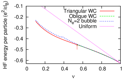
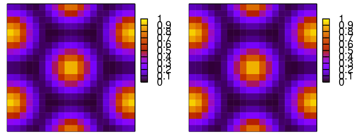
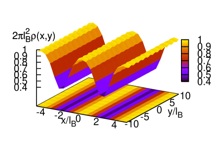
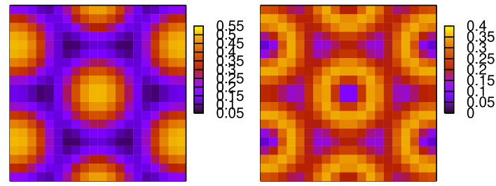
For , the equivalence between single-particle wavefunctions for graphene and conventional 2DEG, implies that at small filling factors, the ground state is a triangular Wigner crystal. Yang et al. (2001) Indeed, graphene, with its pseudospin (valley index) can be mapped onto a bilayer system in which layer index is the pseudospin, in the limit when the layer separation . Our calculations reproduce the results for ground state energy and lattice structure. Figure 1 shows the mean-field energy per particle (phase diagram) as a function of partial filling factor for different lattice structures. We see that for , the ground state is triangular Wigner crystal; it becomes an anisotropic Wigner crystal for . We find that a bubble crystal with is identical, in energy, to the triangular Wigner crystal, and the bubble crystals with have higher energies. Figure 2 shows the real-space electron density profile for graphene at partial filling and for a bilayer quantum Hall system at layer separation at the same filling factor. We obtain, as expected, identical density profiles with a triangular Wigner crystal. As the partial filling is increased, the ground state of the system changes to an anisotropic Wigner crystal (Figure 3). We find, in general, that the optimal value of anisotropy is high. Therefore, the electron density resembles uniform stripe states and the density modulation along the stripes is quite small (Figure 3).
For , the equivalence between graphene and a bilayer quantum Hall system at layer separation breaks down since the single-particle wave functions are different. Figures 4-6 show the phase diagram as a function of partial filling factor for Landau levels =1-3, respectively. The phase diagram of Landau level is qualitatively similar to Landau level. For we find that the ground state for graphene is an isotropic crystal when the partial filling factor is small, whereas it is an anisotropic crystal when is sufficiently large. For intermediate values of , we find that the ground state is a bubble crystal with or . For example, for Landau level in graphene, the triangular Wigner crystal is stable for , the bubble state with two electrons is stable for , whereas for an anisotropic Wigner crystal has the lowest energy. We can also see that the critical values of at which transitions from a triangular Wigner crystal to a bubble state to an anisotropic Wigner crystal take place are systematically higher than corresponding values for a bilayer system at . Figure 7 shows optimal value of for the ground state crystal structure for different Landau level indices. We see that the transition from an isotropic Wigner crystal () to an anisotropic Wigner crystal in graphene (a) occurs at higher values of than the corresponding values in bilayer systems (b).
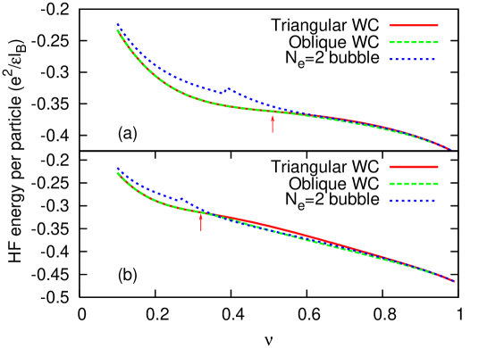
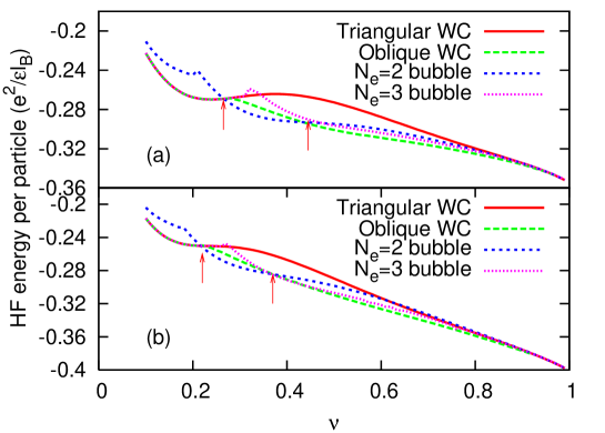
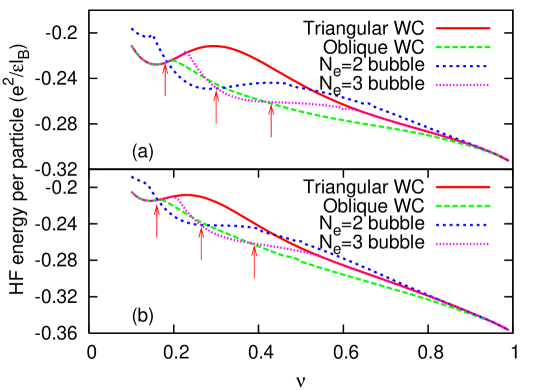
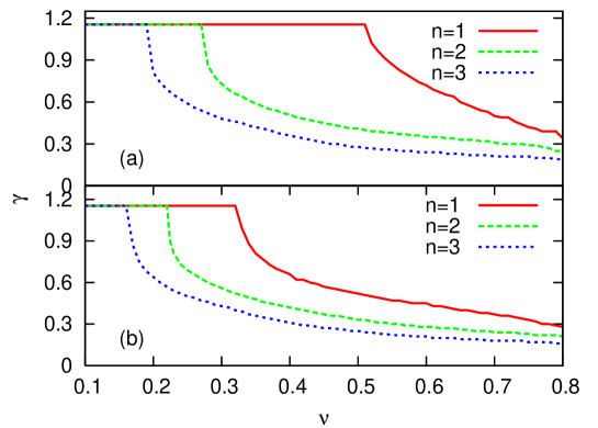
Figure 8 shows the (dimensionless) real-space electron density profile for the Landau level when the system is in the isotropic Wigner crystal state (), in the bubble crystal state with () and with (), and in the anisotropic Wigner crystal state (). We see that the density profile is different from that in the lowest Landau level, due to different form factors. It is instructive to compare density profiles of the anisotropic Wigner crystal in the Landau level and Landau level (Fig. 3). We see that both resemble a (quasi)-uniform striped states, although the density profile also shows the existence of uniform stripes between the modulated ones.
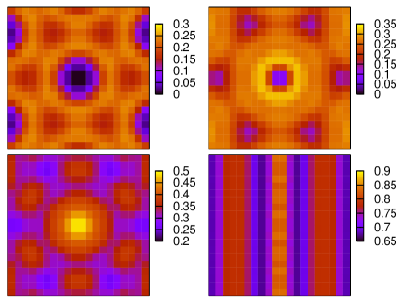
We end this section by comparing the electron density profiles in graphene and bilayer system with at partial filling in the Landau level in Fig. 9. Recall that in the lowest Landau level, these density profiles are identical (Fig 2). For both systems, the self-consistent solutions for the density matrix are identical; however, for , due to the differences in form factors, the resultant real-space electron density profiles are different.
V Discussion and Conclusions
In this paper, we have systematically studied the ground state of graphene in the presence of a strong magnetic field, focusing on broken symmetry states with intervalley coherence, using the Hartree-Fock mean-field analysis. We have ignored the inter-Landau level transitions (since their inclusion does not qualitatively change the phase diagram) and considered spin-split Landau levels. We have focused only states with inter-valley coherence because, due to the isotropic Coulomb interaction,energy of a state without coherence is always larger than the energy of a state with intervalley coherence. Thus, in experiments, these levels will correspond to total filling factors (lowest subband of the level), (lowest subband of the level), (lowest subband of the level). Our calculations, naturally, have also not taken into account competing (Laughlin) fluid states with uniform density. Such fluid states will have lower energy at special filling factors, for example, ; however, our results likely represent the true ground state of the system at generic filling factors and in high Landau levels (where, in a conventional 2DEG, Hartree-Fock solutions are reliable).
Our analysis found that, since the kinetic energy of graphene’s linearly dispersing carriers is quenched in the presence of a magnetic field, graphene is qualitatively similar to a conventional 2DEG with a quantum degree of freedom (bilayer quantum Hall system at or a single layer system with vanishing Zeeman coupling). We showed that the (mean-field) ground state of graphene is evolves from a triangular Wigner crystal to an anisotropic Wigner crystal (striped state) as the partial filling in a given Landau level is increased. We also showed that for Landau level indices , a bubble crystal state with two electrons per unit cell, occurs at intermediate values of . Koulakov et al. (1996) We have compared our results with mean-field results for a corresponding bilayer system at (where the Coulomb interaction becomes isotropic in the pseudospin space). Our findings indicate that different form factors for electrons in graphene systematically shift the critical values of at which the phase transitions occur to higher values, thus expanding the region of stability for the triangular Wigner crystal and bubble crystal states, compared to their counterparts in bilayer systems.
These broken symmetry states in graphene are open to more probes than the conventional 2DEG. Our analysis predicts that anisotropies in the longitudinal resistance will be observed in high Landau levels (similar to those observed in quantum Hall systems) and will provide a signature of highly anisotropic Wigner crystal (striped) states. In addition, since the 2DEG in graphene is literally at the surface, the electron density modulations can be directly probed, by scanning tunneling microscopy, and may provide a direct evidence of electronic crystal states. A weak random disorder will, in general, pin these crystals and destroy the true long-range order. However, since it does not prefer one crystal structure over another, the disorder will not change the phase diagram qualitatively. Direct experimental observation of charge and current density distribution in quantum Hall systems is an outstanding problem; observation of isotropic Wigner crystal and striped states in graphene will improve our understanding of local structure of quantum Hall states.
VI Acknowledgments
It is a pleasure to thank Herb A. Fertig, Sasha Balatsky, and Allan MacDonald for helpful discussions.
References
- Wigner (1934) E. Wigner, Phys. Rev. 46, 1002 (1934).
- Grimes and Adams (1979) C. C. Grimes and G. Adams, Phys. Rev. Lett. 42, 795 (1979).
- Wigner (1989) E. Wigner, Phys. Rev. B 39, 5005 (1989).
- (4) Perspectives in quantum hall effects, edited by Das Sarma and A. Pinczuk (Wiley and Sons, New York, 1997).
- Willett et al. (1988) R. L. Willett, H. L. Stormer, D. C. Tusi, L. N. Pfeiffer, K. W. West, and K. W. Baldwin, Phys. Rev. B 38, 7881 (1988).
- Lilly et al. (1999) M. P. Lilly, K. B. Cooper, J. P. Eisenstein, L. N. Pfeiffer, and K. W. West, Phys. Rev. Lett. 82, 394 (1999).
- Wallace (1947) P. R. Wallace, Phys. Rev. 71, 622 (1947).
- (8) K. S. Novoselov, A. K. Geim, S. V. Morozov, D. Jiang, M. I. Katsnelson, I. V. Grigorieva, S. V. Dubonos and A. A. Firsov, Nature 438, 197 (2005); Yuanbo Zhang, Yan-Wen Tan, Horst L. Stormer and Philip Kim, Nature 428, 201 (2005).
- Dahal et al. (2006) H. P. Dahal, Y. N. Joglekar, K. S. Bedell, and A. V. Balatsky, Phys. Rev. B 74, 233405 (2006).
- Semenoff (1984) G. W. Semenoff, Phys. Rev. Lett. 53, 2449 (1984).
- Haldane (1988) F. D. M. Haldane, Phys. Rev. Lett. 61, 2015 (1988).
- Peres et al. (2005) N. M. R. Peres, F. Guinea, and A. H. C. Neto, Phys. Rev. B 73, 125411 (2005).
- Koulakov et al. (1996) A. A. Koulakov, M. M. Fogler, and B. I. Shklovskii, Phys. Rev. Lett. 76, 499 (1996).
- Goerbig et al. (2004) M. O. Goerbig, P. Lederer, and C. M. Smith, Phys. Rev. B 69, 115327 (2004).
- Côté and Fertig (2000) R. Côté and H. A. Fertig, Phys. Rev. B 62, 1993 (2000).
- Ettouhami et al. (2006) A. M. Ettouhami, C. B. Doiron, F. D. Klironomos, R. Côté, and A. T. Dorsey, Phys. Rev. Lett. 96, 196802 (2006).
- Goerbig et al. (2006) M. O. Goerbig, R. Moessner, and B. Doucot, Phys. Rev. B 74, 161407(R) (2006).
- (18) R. Côté and A. H. Macdonald, Phys. Rev. Lett. 65, 2662(1990); Phys. Rev. B 44, 8759(1991).
- Côté et al. (1992) R. Côté, L. Brey, and A. H. MacDonald, Phys. Rev. B 46, 10 239 (1992).
- Chen and Quinn (1992) X. M. Chen and J. J. Quinn, Phys. Rev. B 45, 11 054 (1992).
- Zhang et al. (2006) Y. Zhang, Z. Jiang, J. P. Small, M. S. Purewal, Y.-W. Tan, M. Fazlollahi, J. D. Chudow, J. A. Jaszczak, H. L. Stormer, and P. Kim, Phys. Rev. Lett. 96, 136806 (2006).
- Brey and Fertig (2000) L. Brey and H. A. Fertig, Phys. Rev. B 62, 10268 (2000).
- Yang et al. (2001) K. Yang, F. D. M. Haldane, and E. H. Rezayi, Phys. Rev. B 64, 081301 (2001).