Kinetic theory of point vortices in two dimensions: analytical results and numerical simulations

Abstract

We develop the kinetic theory of point vortices in two-dimensional hydrodynamics and illustrate the main results of the theory with numerical simulations. We first consider the evolution of the system “as a whole” and show that the evolution of the vorticity profile is due to resonances between different orbits of the point vortices. The evolution stops when the profile of angular velocity becomes monotonic even if the system has not reached the statistical equilibrium state (Boltzmann distribution). In that case, the system remains blocked in a quasi stationary state with a non standard distribution. We also study the relaxation of a test vortex in a steady bath of field vortices. The relaxation of the test vortex is described by a Fokker-Planck equation involving a diffusion term and a drift term. The diffusion coefficient, which is proportional to the density of field vortices and inversely proportional to the shear, usually decreases rapidly with the distance. The drift is proportional to the gradient of the density profile of the field vortices and is connected to the diffusion coefficient by a generalized Einstein relation. We study the evolution of the tail of the distribution function of the test vortex and show that it has a front structure. We also study how the temporal auto-correlation function of the position of the test vortex decreases with time and find that it usually exhibits an algebraic behavior with an exponent that we compute analytically. We mention analogies with other systems with long-range interactions.

1 Introduction

Systems with long-range interactions have been the object of considerable interest in recent years (see different contributions in the book dauxois ). Their dynamics is very rich and presents many interesting features houches ; pa1 . Therefore, the construction of a kinetic theory adapted to such systems is a challenging problem with a lot of potential applications. Several kinetic theories have been developed in the past. The first kinetic theory was constructed by Boltzmann boltzmann for ideal gases. In that case, the particles do not interact except during strong collisions. His results were later extended by Landau landau in the case of Coulombian plasmas and by Chandrasekhar chandra (see a review by Kandrup kandrupREV ) in the case of stellar systems. Developements and improvements of the kinetic theory of Coulombian plasmas were made by Lenard lenard and Balescu balescu using more formal approaches allowing to take into account collective effects. They showed in particular how collective effects can regularize the logarithmic divergence of the diffusion coefficient at the Debye length. More recently, Bouchet & Dauxois bouchet ; bd , Chavanis et al. cvb ; curious and Chavanis & Lemou cl have developed the kinetic theory of the Hamiltonian Mean Field (HMF) model, a toy model of systems with long-range interactions which possesses a lot of interesting properties and which can be studied in great detail. On the other hand, Chavanis pa1 ; landaud and Benedetti et al. benedetti have worked out the kinetic theory of a 2D Coulombian plasma and Valageas valageas has built up a kinetic theory for a 1D gravitational system in a cosmological context. Finally, Chavanis action has obtained a general kinetic equation, written in angle-action variables, which is expected to describes the dynamical evolution of a one-dimensional inhomogeneous system of particles coupled by a weak long-range binary potential of interaction.

In this paper, we shall consider the kinetic theory of point vortices in two-dimensional hydrodynamics houches . In that case, the particles interact via a logarithmic potential in two dimensions. The dynamical evolution of the system is due to long-range collisions which involve interactions between vortices that can be at large distances from each others (this will be referred to as “distant collisions”). The point vortex gas is probably the first physical system for which long-range interactions and spatial delocalization play a prevalent role in the kinetic theory. Indeed, it is not possible to assume that the system is spatially homogeneous as done in the kinetic theory of Coulombian plasmas (invoking Debye shielding ichimaru ), in the kinetic theory of stellar systems (invoking a local approximation bt ), and for the HMF model (above the critical energy $E_{c}$ where a stable homogeneous phase exists [10-12,14]). Furthermore, the point vortex gas is peculiar because point vortices have no inertia so that the collision term in the kinetic equation directly acts in position space. Therefore, the role of position plays the role of velocity in usual kinetic theories. This makes the case of point vortices intermediate between kinetic theories of spatially homogeneous systems for which the evolution occurs only in velocity space [4-12,14-16] and kinetic theories of spatially inhomogeneous systems for which the evolution occurs in velocity and position space curious , or in energy space if we average over the orbits valageas ; action . Because of its connections with other systems with long-range interactions, the kinetic theory of point vortices has a broader interest than simply fluid mechanics.

A kinetic theory of point vortices in a shear flow has been first developed by Nazarenko & Zakharov zac . They considered a multi-components system and assumed that the interaction between vortices is shielded due to geophysical effects like rotation. They studied in detail the close collisions between two-screened particles (Stuart vortices) which are moved to each other by the collective shear flow and developed a kinetic theory à la Boltzmann. They showed that the mean vorticity profile does not change in time and that, due to collisions, the most intensive vortices are concentrated in the regions of large total vorticity while less intensive vortices are in small vorticity regions. For a single species system, the collision integral cancels out identically.

A kinetic theory of point vortices with equal circulation has been developed more recently by Chavanis [22-24,2] (see also related works in Chavanis & Sire cs ; cs2 ) by analogy with the Brownian theory of Chandrasekhar chandraB in stellar dynamics. In a first paper preR , he considered the relaxation of a test vortex in a “sea” of field vortices and derived a Fokker-Planck equation where the evolution of the distribution function of the test vortex is due to the competition between a diffusion term and a drift term. The diffusion arises from the fluctuations of the velocity created by the field vortices and the drift term is due to the response of the field vortices to the perturbation caused by the test vortex, as in a polarization process. Chavanis preR calculated the expression of the diffusion coefficient from the Kubo formula and the expression of the drift term from a linear response theory. This is similar to the calculations of Kandrup kandrup2 in stellar dynamics to determine the diffusion coefficient and the friction force experienced by a test star in a cluster of field stars. It is found that the diffusion coefficient of point vortices is proportional to the local vorticity created by the field vortices and inversely proportional to the shear. On the other hand, the drift velocity is proportional to the local vorticity gradient and inversely proportional to the shear. Assuming that the vorticity profile of the field vortices is positive, axisymmetric and decreasing with the distance, the expression of the drift velocity shows that a test vortex with positive circulation climbs the vorticity gradient and that a test vortex with negative circulation descends the vorticity gradient. When the field vortices have the Boltzmann distribution of statistical equilibrium (thermal bath), the diffusion coefficient and the drift coefficient (mobility) are related to each other by a generalization of the Einstein relation involving a negative temperature. In a second paper, Chavanis kin developed a more complete kinetic theory of point vortices by using the projection operator formalism of Willis & Picard wp . From this general formalism, he obtained a kinetic equation describing the evolution of the vortex system “as a whole”. This is the counterpart of the generalized Landau equation obtained by Kandrup kandrup1 in stellar dynamics. This equation conserves the energy and monotonically increases the Boltzmann entropy ($H$-theorem). The computed collision integral is of order $O(1/N)$ in a proper thermodynamic limit $N\rightarrow+\infty$ where the domain area $V$ is fixed and the circulation of the point vortices scales like $\gamma\sim 1/N$ (so that the total circulation $\Gamma=N\gamma$ is of order unity). This collision integral takes into account the influence of two-body correlations. For $N\rightarrow+\infty$, the correlations are negligible and we recover the 2D Euler equation which describes a “collisionless” evolution. This is the counterpart of the Vlasov equation in plasma physics. At order $O(1/N)$, the kinetic theory shows that the “collisional” evolution is due to a condition of resonance between the trajectories of point vortices that can be far away. Therefore, this approach takes into account distant collisions between vortices while the approach developed by Nazarenko & Zakharov zac focuses on close collisions. This is why the collision integral derived in kin can be non-zero for a single species system of vortices while it cancels out identically in zac . The above-mentioned kinetic theory, developed at the order $O(1/N)$, describes the evolution of the system on a timescale of order $Nt_{D}$, were $t_{D}$ is the dynamical time. Furthermore, it assumes that the point vortices are transported by the collective shear flow (meanfield velocity) rather than, say, triple collisions. It is valid therefore when the shear is sufficiently strong in the system. If we implement a thermal bath approximation to describe the relaxation of a test vortex in a fixed distribution of field vortices, we recover the Fokker-Planck equation involving the terms of diffusion and drift obtained in preR . In that case, the relaxation time scales like $(N/\ln N)t_{D}$.

Similar problems have been studied independently by Dubin and collaborators [31-34] in the context of non-neutral plasmas under a strong magnetic field, a system isomorphic to the point vortex system. Dubin & O’Neil dn developed a kinetic theory of these systems, starting from the Klimontovich equation pitaevskii and using methods of plasma physics. Their kinetic theory is able to take into account collective effects that are ignored in the approach of Chavanis kin . However, the kinetic equation obtained by Chavanis kin captures the main properties of the dynamics and can be solved numerically more easily, an advantage that will be used in the present paper. In recent works, Dubin and collaborators [32-34] studied the dynamics of a test vortex in a background shear and provided very nice numerical simulations and laboratory experiments of this process. On a theoretical point of view, they derived the expressions of the diffusion coefficient and of the drift velocity of the test vortex. These expressions are consistent with those obtained previously by Chavanis preR ; kin . They also addressed the form of the cut-off to the logarithmic divergence that occurs in these quantities. However, they introduced these terms of diffusion and drift as independent effects and did not derive the Einstein relation connecting the diffusion to the drift nor the Fokker-Planck equation governing the evolution of a test vortex in a fixed distribution of field vortices.

The object of the paper is to further develop the kinetic theory of point vortices and numerically solve the corresponding kinetic equations in order to illustrate the basic results of the theory. The kinetic theory is important to describe the relaxation of the system towards the Boltzmann distribution predicted by equilibrium statistical mechanics for $t\rightarrow+\infty$ [36-41]. It is also necessary to determine the timescale of the collisional relaxation and to prove whether or not the system will truly relax towards Boltzmann statistical equilibrium. Indeed, the convergence towards Boltzmann statistical equilibrium, which is based on an assumption of ergodicity, is not firmly established for complex systems with long-range interactions such as point vortices. A first reason is that such systems exhibit non-markovian effects and spatial delocalization so that the monotonic increase of the Boltzmann entropy is difficult to prove and could even be wrong in a strict sense kin . It is only when additional approximations are included (markovian approximation, neglect of three-body correlations,..) that the Boltzmann $H$-theorem is recovered . On the other hand, the evolution of the system is due to resonances between different orbits and it may happen that the evolution stops before the system has reached statistical equilibrium because there is no resonance anymore. In that case, the system is blocked in a quasi stationary state (QSS) which can persist for a very long time. One object of the paper is to discuss these issues and perform numerical simulations in order to illustrate the particularity of the point vortex dynamics.

The paper is organized as follows. In Sec. 2, we briefly discuss the statistical mechanics of the point vortex gas at equilibrium and extend the theory to the case where the point vortices have different circulations. The predictions of equilibrium thermodynamics will be compared with the results of the kinetic theory throughout the paper. In Sec. 3, we develop the kinetic theory of point vortices and describe the evolution of the system “as a whole”. In Sec. 3.1, we generalize the kinetic theory of kin , based on the projection operator formalism, to a multi-species point vortex gas. Considering an axisymmetric evolution, we obtain an explicit kinetic equation for the evolution of the system at the order $O(1/N)$. We provide a simpler derivation of this kinetic equation than the one given in kin . We also stress some technical difficulties associated with the kinetic theory and propose some solutions to circumvent these problems. In Sec. 3.3, we show that the derived kinetic equation conserves the vortex number of each species, the total energy and the total angular momentum. Furthermore, it increases the Boltzmann entropy ($H$-theorem). For a single species system, the evolution of the point vortex gas on a timescale $Nt_{D}$ is due to a condition of resonance $\Omega(r,t)=\Omega(r^{\prime},t)$ between different orbits $r\neq r^{\prime}$ that can be satisfied only when the profile of angular velocity is non-monotonic. As a result, the Boltzmann distribution corresponding to statistical equilibrium is not the only stationary solution of the kinetic equation. For example, any distribution with a monotonic profile of angular velocity is a steady state solution. Therefore, the dynamical evolution stops when the profile of angular velocity becomes monotonic even if the system has not reached the Boltzmann distribution (further evolution may occur on longer timescale due to terms of order $1/N^{2}$, $1/N^{3}$…, in the kinetic theory corresponding to the influence of three-body, or higher, correlations). This kinetic blocking, described in Sec. 3.2, is illustrated numerically in Sec. 3.4. In Sec. 4, we consider the relaxation of a test vortex in a bath of field vortices. In Sec. 4.1, we show that the stochastic process is described by a Fokker-Planck equation involving a term of diffusion and a term of drift. This Fokker-Planck equation can be derived from the projection operator formalism. We extend the approach of kin by considering a test particle with a circulation $\Gamma_{0}$ that can be different from the circulation $\gamma$ of the field particles. In Sec. 4.2, we discuss specifically the terms of diffusion and drift. For a thermal bath of field vortices, we show that they are related to each other by a generalized Einstein relation $\xi=D\beta\Gamma_{0}$. Furthermore, the diffusion coefficient $D(r)$ depends on the position and decreases rapidly with the distance, leading to anomalous dynamical behaviors. In Sec. 4.3, we derive the first and second moments of the radial position increment from the Fokker-Planck equation. In Appendix C, we directly compute these moments from the Hamiltonian equations of motion. We can therefore justify the Fokker-Planck equation by this alternative approach instead of advocating the projection operator formalism. In Sec. 4.4, we precisely discuss the scaling of the relaxation time with $N$. We distinguish the collisional timescale $\sim Nt_{D}$ associated with the evolution of the system “as a whole” from the collisional timescale $(N/\ln N)t_{D}$ associated with the evolution of a test vortex in a bath. In Sec. 5, we consider different features of the Fokker-Planck equation. In Sec. 5.1, we study the evolution of the tail of the distribution function of the test vortex and show that it has a front structure. We characterize the displacement of the front and its shape. In Sec. 5.2, we consider the temporal auto-correlation function of the position of the test vortex and show that, in cases of physical interest, it decreases algebraically with time. The exponent of algebraic decay is computed analytically and compared with direct numerical simulations. In Secs. 6 and 7, we consider explicit examples of Fokker-Planck equations corresponding to typical bath distributions of the field vortices. In order to be complete, we describe various examples of flow profiles. However, we present numerical simulations only for the gaussian vortex.

2 The point vortex gas at equilibrium

2.1 The statistical equilibrium state

Basically, the dynamical evolution of a system of point vortices in two dimensions is described by the Hamiltonian equations of motion newton :

$$\gamma_{i}{dx_{i}\over dt}={\partial H\over\partial y_{i}},\qquad\gamma_{i}{dy_{i}\over dt}=-{\partial H\over\partial x_{i}},$$ (1)

$$H=-{1\over 2\pi}\sum_{i<j}\gamma_{i}\gamma_{j}\ln|{\bf r}_{i}-{\bf r}_{j}|,$$ (2)

where $\gamma_{i}$ is the circulation of point vortex $i$. A particularity of this Hamiltonian system, first noticed by Kirchhoff kirchhoff , is that the coordinates $(x,y)$ of the point vortices are canonically conjugate. The point vortex system conserves several quantities. The number $N_{a}$ of vortices of species $a$, or equivalently the total circulation of each species $\Gamma_{a}=N_{a}\gamma_{a}$, is conserved. The system also conserves the energy $E=H$. There are additional conserved quantities depending on the geometry of the domain. The angular momentum $L=\sum_{i}\gamma_{i}r_{i}^{2}$ is conserved in an infinite domain or in a disk and the linear impulse ${\bf P}=\sum_{i}\gamma_{i}{\bf r}_{i}$ is conserved in an infinite domain or in a channel. In an unbounded domain, we must consider vortices of the same circulation otherwise they would form pairs (dipoles) and escape to infinity, so there is no equilibrium. In a bounded domain, the Hamiltonian has to be modified so as to take into account the contribution of vortex images. Note that the Hamiltonian (2) does not involve a kinetic term $\sum_{i}m_{i}v_{i}^{2}/2$ usually present for material particles. This is because point vortices have no inertia. Therefore, a point vortex produces a velocity, not an acceleration (or a force), contrary to other systems of particles in interaction like electric charges in a plasma landau or stars in a galaxy chandra . In a sense, this interaction is related to the conception of motion according to Descartes, in contrast to Newton.

Assuming ergodicity, the point vortex gas is expected to achieve a statistical equilibrium state for $t\rightarrow+\infty$. The statistical mechanics of point vortices is very peculiar and was first discussed by Onsager onsager . He considered box-confined configurations and showed that for sufficiently large energies, point vortices of the same sign tend to “attract” each other and group themselves to form “clusters” or “supervortices” similar to the large-scale vortices observed in the atmosphere of giant planets. When all the vortices have the same sign, this leads to monopoles (cyclones or anticyclones) and when vortices have positive and negative signs, this leads to dipoles (a pair of cyclone/anticlone) or even tripoles. These organized states are characterized by negative temperatures. This is due to the fact that the structure function $\Phi(E)=\int_{H\leq E}dx_{1}dy_{1}...dx_{N}dy_{N}$ is finite for $E\rightarrow+\infty$ since the phase space coincides with the configuration space: $\Phi(+\infty)=\int dx_{1}dy_{1}...dx_{N}dy_{N}=V^{N}$ where $V$ is the area of the system. The existence of negative temperatures for point vortices should not cause surprise. For material particles, the temperature is a measure of the velocity dispersion and it must be positive. Indeed, it appears in the Maxwell distribution $e^{-\beta v^{2}/2}$ (or in the partition function) which can be normalized only for $\beta>0$. However, since point vortices have no inertia, there is no such term in the equilibrium distribution of point vortices (see below) and the temperature can be negative.

To obtain more quantitative results, Joyce & Montgomery jm and Lundgren & Pointin lp considered a mean field approximation. This is valid in a proper thermodynamic limit $N\rightarrow+\infty$ in such a way that the normalized temperature $\eta=\beta N\gamma^{2}$ and the normalized energy $\epsilon=E/N^{2}\gamma^{2}$ are fixed (for a single species system). On physical grounds, it is reasonable to consider that the area of the domain and the total circulation of the vortices are of order unity. Then, by rescaling the parameters appropriately, the proper thermodynamic limit corresponds to $N\rightarrow+\infty$ with $\gamma\sim 1/N$, $V\sim 1$, $E\sim 1$ and $\beta\sim N$ houches . Since the coupling constant $\beta\gamma^{2}=\eta/N\sim 1/N$ goes to zero for $N\rightarrow+\infty$, we are considering a weak long-range potential of interaction. In that limit, we can neglect the correlations between vortices and the statistical equilibrium distribution of point vortices is given by the Boltzmann distribution

$$P_{eq}({\bf r})=Ae^{-\beta\gamma\psi({\bf r})},$$ (3)

where $\psi$ is the stream function. Using the Poisson equation $\Delta\psi=-\omega$ with the smooth vorticity $\omega({\bf r})=N\gamma P({\bf r})$, the statistical equilibrium state is obtained by solving the Boltzmann-Poisson equation

$$-\Delta\psi=N\gamma Ae^{-\beta\gamma\psi},$$ (4)

and substituting the resulting stream function in Eq. (3). Joyce & Montgomery jm obtained the equilibrium distribution (3) by maximizing the entropy of the point vortex gas at fixed circulation and energy. Lundgren & Pointin lp derived Eq. (4) from the equilibrium BBGKY hierarchy of equations in the limit $N\rightarrow+\infty$. A rigorous derivation of the mean field equations was provided by [39-41].

On the other hand, at sufficiently large negative energies, the temperature is positive. In that case, like-sign vortices tend to “repell” each other. When all the vortices of the system have the same sign, they accumulate on the boundary of the domain. This regime can again be described by the mean field theory of [37-41]. Alternatively, when the system is neutral, opposite-sign vortices tend to “attract” each other resulting in a spatially homogeneous distribution with strong correlations between vortices. In that case, the point vortex gas is similar to a Coulombian plasma. This is the situation considered by Fröhlich & Ruelle fr . As discussed by Ruelle ruelle , we may expect a phase transition (related to the Kosterlitz-Thouless transition) as a function of the temperature. At large (positive) temperatures, the system is in a “conducting phase” (in the plasma analogy) with free vortices that can screen external “charges”. In that case, there can be Debye shielding like for a Coulombian plasma. At low (positive) temperatures, opposite-sign vortices tend to form pairs $(+,-)$ and the gas is in a “dielectric phase” where all charges are bound forming dipolar pairs. These “dipoles” are similar to “atoms” $(+e,-e)$ in plasma physics. In that case, there is no screening.

Summarizing, there are two very different regimes in the point vortex gas that correspond to different thermodynamic limits. In the meanfield theory of [37-41], the thermodynamic limit corresponds to $N\rightarrow+\infty$ in such a way that the size $V$ of the system is fixed and the interaction between vortices is weak since the “charge” of the vortices tends to zero as $\gamma\sim 1/N$. In that case, the system is spatially inhomogeneous, the correlations between vortices are negligible for $N\rightarrow+\infty$, there is no shielding and the temperature can be negative. The physics of the problem is controlled by the one-body distribution function $P({\bf r})$. Alternatively, Fröhlich & Ruelle fr consider a neutral system of $2N$ positive and negative point vortices with circulation $\pm\gamma$ and take the usual thermodynamic limit $N,V\rightarrow+\infty$ with $N/V$ and $E/N$ fixed (with $\gamma\sim 1$). In that case, the system is spatially homogeneous in average, the temperature is positive and the physics of the problem is controlled by the two-body correlation function. In the screening phase (at high positive temperatures), there is Debye shielding and the correlation function tends to zero exponentially rapidly.

2.2 Generalization to a collection of circulations

In this paper, we shall restrict ourselves to the situation described in [37-41]. In this section, we generalize the maximum entropy method of Joyce & Montgomery jm in order to determine the statistical equilibrium state of a system of point vortices with different circulations. This will be useful to interpret the results of Sec. 3.2. Following the Boltzmann procedure, we divide the domain into a very large number of microcells with size $h^{2}$ (ultimately $h\rightarrow 0$). A microcell can be occupied by an arbitrary number of point vortices. We shall now group these microcells into macrocells each of which contains many microcells but remains nevertheless small compared to the extension of the whole system. We call $\nu$ the number of microcells in a macrocell. A macrostate is specified by the number $\{n_{ia}\}$ of point vortices of circulation $\gamma_{a}$ in the macrocell $i$ (irrespective of their position in the cell) while a microstate is specified by their precise position in the cell. Using a combinatorial analysis, the number of microstates corresponding to the macrostate $\{n_{ia}\}$ is

$$W(\{n_{ia}\})=\prod_{a}N_{a}!\prod_{i}\frac{\nu^{n_{ia}}}{n_{ia}!}.$$ (5)

We introduce $n_{a}({\bf r})$ the smooth density of point vortices of species $a$ in ${\bf r}$. The vorticity of species $a$ is then $\omega_{a}({\bf r})=\gamma_{a}n_{a}({\bf r})$. If we define the Boltzmann entropy by $S=\ln W$, use the Stirling formula for $n_{ia}\gg 1$ and take the continuum limit, we get

$$S=-\sum_{a}\int{\omega_{a}\over\gamma_{a}}\ln{\omega_{a}\over\gamma_{a}}\ d{\bf r}.$$ (6)

The Boltzmann entropy (6) measures the number of microstates corresponding to the macrostate specified by $\{\omega_{a}({\bf r})\}$. At statistical equilibrium, the system is expected to be in the most probable macrostate, i.e. the one that is the most represented at the microscopic level. Assuming that all the microstates are equiprobable, the equilibrium distribution is obtained by maximizing the Boltzmann entropy (6) while conserving the circulation of each species $\Gamma_{a}=\int\omega_{a}d{\bf r}$ and the mean field energy $E={1\over 2}\int\omega\psi d{\bf r}$. The vorticity and the streamfunction are related to each other by the Poisson equation

$$-\Delta\psi=\omega=\sum_{a}\omega_{a}.$$ (7)

Finally, in an infinite domain or in a disk, we must also conserve the angular momentum $L=\int\omega r^{2}d{\bf r}$. Introducing Lagrange multipliers and writing the first order variations as

$$\delta S-\sum_{a}\alpha_{a}\delta\Gamma_{a}-\beta\delta E-{1\over 2}\beta\Omega_{L}\delta L=0,$$ (8)

we find that the most probable state is

$$\omega_{a}({\bf r})=A_{a}e^{-\beta\gamma_{a}\psi^{\prime}({\bf r})},$$ (9)

where

$$\psi^{\prime}=\psi+{1\over 2}\Omega_{L}r^{2},$$ (10)

is the relative stream function. This describes a flow that is steady in a frame rotating with angular velocity $\Omega_{L}$ (see Appendix A). Therefore, the equilibrium state is obtained by solving the multi-species Boltzmann-Poisson equation

$$-\Delta\psi=\sum_{a}A_{a}e^{-\beta\gamma_{a}\psi^{\prime}({\bf r})},$$ (11)

and substituting the resulting stream function back into Eq. (9). The Lagrange multipliers can then be related to the integral constraints. We note that the vorticity profiles of different species are related to each other by

$$\left({\omega_{a}\over A_{a}}\right)^{1/\gamma_{a}}=\left({\omega_{b}\over A_{b}}\right)^{1/\gamma_{b}},$$ (12)

hence

$$\omega_{a}({\bf r})=C_{ab}|\omega_{b}({\bf r})|^{\gamma_{a}/\gamma_{b}},$$ (13)

where $C_{ab}$ is independent on the position. Assuming that $\gamma_{a}>0$, $\gamma_{b}>0$ and that $\omega_{b}({\bf r})$ decreases with the distance (which corresponds to equilibrium states with $\beta<0$), this relation indicates that intense vortices ($\gamma_{a}>\gamma_{b}$) are more concentrated at the center, on average, than weaker vortices. On the other hand, Eq. (13) shows that opposite sign vortices tend to separate (at negative temperatures where the mean field theory applies). More generally, Eq. (13) characterizes the seggregation between vortices with different circulations.

3 Evolution of the system as a whole

The equilibrium statistical mechanics tells nothing concerning the timescale of the relaxation towards statistical equilibrium. It is furthermore not obvious whether the system of point vortices will truly relax towards statistical equilibrium or not. Indeed, the Boltzmann distribution (3) is based on a hypothesis of ergodicity and on the assumption that all the accessible microstates are equiprobable. This is essentially a postulate. In order to precisely answer these questions we need to develop a kinetic theory of point vortices.

3.1 Kinetic theory of point vortices

There are different methods to obtain a kinetic equation for a system of point vortices. One approach is to start from the Klimontovich equation and develop a quasi-linear theory as in plasma physics dn . Another possibility is to start from the Fokker-Planck equation and calculate the first $\langle\Delta r\rangle$ and second moments $\langle(\Delta r)^{2}\rangle$ of the increments of position of a point vortex due to the interaction with the other vortices. This approach is developed in Appendix C. A third possibility is to start from the Liouville equation and use the projection operator formalism kin . An interest of this formalism is to yield a general non-Markovian equation that is valid for flows that are not necessarily axisymmetric. The other formalisms assume from the begining that the distribution of point vortices is axisymmetric and work in Fourier space (for the angular variables). By contrast, the projection operator formalism remains in physical space which enlightens the basic physics. Indeed, even if the formalism is abstract and complicated wp , the final kinetic equation takes a rather nice form which bears a clear physical meaning . The drawback of that approach is that it ignores collective effects. For axisymmetric flows, these collective effects have been taken into account in the approach of Dubin & O’Neil dn .

We shall here extend the kinetic theory of Chavanis kin , based on the projection operator formalism, to the case of a multi-components point vortex gas. We shall not repeat the intermediate steps of the calculations that can be found in kin . Generalizing these calculations in order to include a distribution of circulations among the point vortices, we obtain a kinetic equation of the form

$${\partial\omega_{a}\over\partial t}+\langle{\bf V}\rangle\cdot\nabla\omega_{a}={\partial\over\partial r^{\mu}}\sum_{b}\int_{0}^{t}d\tau\int d{\bf r}_{1}{\cal V}^{\mu}(1\rightarrow 0)$$

$$\times{\cal G}(t,t-\tau)\biggl{[}\gamma_{b}{\cal V}^{\nu}(1\rightarrow 0){\partial\over\partial r^{\nu}}$$

$$+\gamma_{a}{\cal V}^{\nu}(0\rightarrow 1){\partial\over\partial r_{1}^{\nu}}\biggr{]}\omega_{a}({\bf r},t-\tau)\omega_{b}({\bf r}_{1},t-\tau),$$

(14)

where ${\cal G}(t,t-\tau)$ is the Green function associated with the averaged Liouville operator constructed with the mean field velocity $\langle{\bf V}\rangle({\bf r},t)=-{\bf z}\times\nabla\psi$. In words, this means that we must perform the time integration by moving the point vortices between $t$ and $t-\tau$ with the mean field velocity. On the other hand, ${\cal V}^{\mu}(1\rightarrow 0,t)={V}^{\mu}(1\rightarrow 0,t)-\langle V^{\mu}\rangle({\bf r},t)$ is the fluctuating velocity by unit of circulation created by particle $1$ located in ${\bf r}_{1}$ on particle $0$ located in ${\bf r}$ (see Appendix B). To obtain this closed kinetic equation, we have implicitly assumed that three-body correlations are negligible. This neglect is valid at order $1/N$ in the proper thermodynamic limit $N\rightarrow+\infty$ defined above. In the general kinetic equation (14), we clearly see the terms of diffusion and drift (first and second terms in the r.h.s.) and their connection to a generalized form of Kubo formula (the integral over time of the velocity auto-correlation function). These points will be further developed in the sequel. The ratio of the “collision” term (right hand side) on the advective term (left hand side) is of order $1/N$ in the thermodynamic limit (see Sec. 4.4). Therefore, this kinetic equation is valid at order $O(1/N)$ in an expansion of the collision term in powers of $1/N$. Thus, it describes the evolution of the system on a timescale of the order $Nt_{D}$ where $t_{D}$ is the dynamical time.

We must distinguish two regimes in the evolution of the point vortex system:

(i) Collisionless regime: For fixed $t$ and $N\rightarrow+\infty$, the collision term on the r.h.s. of Eq. (14) vanishes and this equation reduces to the 2D Euler equation kin :

$${\partial\omega_{a}\over\partial t}+\langle{\bf V}\rangle\cdot\nabla\omega_{a}=0.$$ (15)

This is the counterpart of the Vlasov equation in plasma physics ichimaru or stellar dynamics bt (it is valid for each species of particles). It can be directly derived from the Liouville equation by neglecting correlations between vortices, i.e. by assuming that the $N$-body distribution function is a product of $N$ one-body distribution functions kin . The Euler equation (15) describes the collisionless evolution of the point vortex system on a timescale $t\ll Nt_{D}$ where $t_{D}$ is the dynamical time. For $N\gg 1$, the validity of the Vlasov regime can be very long in practice. Starting from an unstable initial condition, the 2D Euler-Poisson system can undergo a “violent relaxation” driven by purely mean field effects houches . This form of collisionless relaxation leads to the rapid emergence of a quasi stationary state (QSS) on the coarse-grained scale [47-50].

(ii) Collisional regime: The “collision” term (right hand side in Eq. (14)) takes into account finite $N$ effects. It can be viewed as the first order correction of the Euler/Vlasov equation in an $N^{-1}$ expansion (see, e.g., houches p. 260). Therefore, the collision term in the kinetic equation (14) manifests itself on a timescale $\sim Nt_{D}$. In this paper, we shall be essentially interested by this “slow collisional evolution”.

In the following, we shall assume that the vorticity profile is a stable stationary solution of the 2D Euler equation, so that it evolves under the sole effect of collisions (finite $N$ effects) on a timescale $Nt_{D}$. Therefore, we shall not describe the process of violent relaxation [47-50] due to mean field effects that takes place during the collisionless regime on a timescale $t_{D}$ (see the Conclusion for a discussion of the different regimes of the dynamics). We thus start from a stable stationary solution of the 2D Euler equation (possibly resulting from a phase of violent relaxation) and discuss its collisional evolution. If we restrict ourselves to axisymmetric flows, the kinetic equation (14) becomes

$${\partial\omega_{a}\over\partial t}={1\over r}{\partial\over\partial r}r\sum_{b}\int_{0}^{t}d\tau\int d{\bf r}_{1}{V}_{r}(1\rightarrow 0,t)$$

$$\times\biggl{[}\gamma_{b}{V}_{r}(1\rightarrow 0,t-\tau){\partial\over\partial r}+\gamma_{a}{V}_{r_{1}}(0\rightarrow 1,t-\tau){\partial\over\partial r_{1}}\biggr{]}$$

$$\times\omega_{a}({r},t-\tau)\omega_{b}({r}_{1},t-\tau),\qquad\qquad$$ (16)

where $V_{r}={\bf V}\cdot\hat{\bf r}$ is the radial component of the velocity in the direction $\hat{\bf r}={\bf r}/r$ of particle $0$ (we adopt the same convention for particle $1$). Since the collision term is of order $1/N$, the smooth distribution $\omega_{a}(r,t)$ evolves on a timescale of order $Nt_{D}$ at least, which is much larger than the timescale on which the fluctuations have essential correlations. Thus, we can make a Markov approximation $\omega({r},t-\tau)\simeq\omega({r},t)$ and extend the time integral to $+\infty$ (see, however, the end of this section). In the same order of approximations, we can consider that, to leading order in $1/N$, the point vortices follow circular trajectories given by

$$r(t-\tau)=r,\qquad\theta(t-\tau)=\theta-\Omega(r,t)\tau,$$ (17)

where $(r,\theta)$ specify the position of a point vortex at time $t$ and $\Omega(r,t)=\langle V\rangle_{\theta}(r,t)/r$ is the angular velocity corresponding to the mean field velocity $\langle V\rangle_{\theta}(r,t)$. Within these approximations, the kinetic equation (16) becomes

$${\partial\omega_{a}\over\partial t}={1\over r}{\partial\over\partial r}r\sum_{b}\int_{0}^{+\infty}d\tau\int d{\bf r}_{1}{V}_{r}(1\rightarrow 0,t)$$

$$\times\biggl{[}\gamma_{b}{V}_{r}(1\rightarrow 0,t-\tau){\partial\over\partial r}+\gamma_{a}{V}_{r_{1}}(0\rightarrow 1,t-\tau){\partial\over\partial r_{1}}\biggr{]}$$

$$\times\omega_{a}({r},t)\omega_{b}({r}_{1},t),\qquad\qquad$$ (18)

where (see Appendix B)

$$V_{r}(1\rightarrow 0,t)=-{1\over 2\pi}{r_{1}\sin(\theta-\theta_{1})\over r_{1}^{2}+r^{2}-2rr_{1}\cos(\theta-\theta_{1})},$$ (19)

$$V_{r}(1\rightarrow 0,t-\tau)=-{1\over 2\pi}{r_{1}\sin(\theta-\theta_{1}-\Delta\Omega\tau)\over r_{1}^{2}+r^{2}-2rr_{1}\cos(\theta-\theta_{1}-\Delta\Omega\tau)},$$

(20)

with $\Delta\Omega=\Omega(r,t)-\Omega(r_{1},t)$. Since ${V}_{r_{1}}(0\rightarrow 1)=-(r/r_{1}){V}_{r}(1\rightarrow 0)$, we can rewrite the foregoing equation in the form

$${\partial\omega_{a}\over\partial t}={1\over r}{\partial\over\partial r}r\sum_{b}\int_{0}^{+\infty}d\tau\int_{0}^{2\pi}d\theta_{1}\int_{0}^{+\infty}rr_{1}d{r}_{1}{V}_{r}(1\rightarrow 0,t)$$

$$\times{V}_{r}(1\rightarrow 0,t-\tau)\biggl{(}\gamma_{b}{1\over r}{\partial\over\partial r}-\gamma_{a}{1\over r_{1}}{\partial\over\partial r_{1}}\biggr{)}\omega_{a}({r},t)\omega_{b}({r}_{1},t).$$

(21)

The kinetic equation involves the function

$$M=\int_{0}^{+\infty}d\tau\int_{0}^{2\pi}d\theta_{1}{V}_{r}(1\rightarrow 0,t){V}_{r}(1\rightarrow 0,t-\tau).\qquad$$ (22)

Using Eqs. (19)-(20), it is shown in kin ; houches (see also Appendix B) that

$$M=-{1\over 4r^{2}}\delta(\Delta\Omega)\ln\biggl{[}1-\biggl{(}{r_{<}\over r_{>}}\biggr{)}^{2}\biggr{]},$$ (23)

where $r_{<}$ (resp. $r_{>}$) denotes the smallest (resp. largest) of $r$ and $r_{1}$. Therefore, the final form of the kinetic equation is

$${\partial\omega_{a}\over\partial t}=-{1\over 4r}{\partial\over\partial r}\sum_{b}\int_{0}^{+\infty}r^{\prime}d{r}^{\prime}\delta(\Omega-\Omega^{\prime})\ln\biggl{[}1-\biggl{(}{r_{<}\over r_{>}}\biggr{)}^{2}\biggr{]}$$

$$\times\biggl{(}\gamma_{b}\omega_{b}^{\prime}{1\over r}{\partial\omega_{a}\over\partial r}-\gamma_{a}\omega_{a}{1\over r^{\prime}}{\partial\omega^{\prime}_{b}\over\partial r^{\prime}}\biggr{)},\qquad\qquad$$ (24)

where $\omega^{\prime}$ stands for $\omega(r^{\prime},t)$ and $\Omega^{\prime}$ stands for $\Omega(r^{\prime},t)$. This generalizes the kinetic equation obtained by Chavanis kin for a single species of point vortices. The angular velocity and the vorticity are expressed in terms of the orthoradial velocity by

$$\langle V\rangle_{\theta}=-{\partial\psi\over\partial r}=\Omega r,\qquad\omega={1\over r}{\partial\over\partial r}(r\langle V\rangle_{\theta}),$$ (25)

so that

$$\omega={1\over r}{\partial\over\partial r}(r^{2}\Omega).$$ (26)

For future convenience, it will be useful to write the logarithm as

$$\ln\biggl{[}1-\biggl{(}{r_{<}\over r_{>}}\biggr{)}^{2}\biggr{]}=-\sum_{n=1}^{+\infty}{1\over n}\biggl{(}{r_{<}\over r_{>}}\biggr{)}^{2n}.$$ (27)

We note that, for a multi-species system, a logarithmic divergence $\sum_{n=1}^{+\infty}1/n$ appears in the kinetic equation (24) when $r^{\prime}=r$ and $b\neq a$. This problem will be discussed specifically in Sec. 4.1. We shall heuristically regularize the divergence by introducing an upper cut-off $\Lambda$ in the series (27) when necessary, writing $\sum_{n=1}^{\Lambda}{1\over n}({r_{<}/r_{>}})^{2n}$.

We also emphasize that the Dirac function arising in Eq. (24) does not make sense for values of $r$ and $r^{\prime}$ such that $\Omega(r)=\Omega(r^{\prime})$ and $(\partial\Omega/\partial r)(r^{\prime})=0$ (in that case, the identity (52) clearly breaks down). Mathematically speaking, the “function” $x\rightarrow\delta(x^{2})$ has no sense even in the space of distributions. To overcome this problem, we can notice that this Dirac distribution comes out formally from Eq. (22) where the time integration takes over all the interval $[0,+\infty)$. Therefore, one could expect that if the time averaging is taken on a finite interval $[0,t)$ only, as in the initial integral (16), then the resulting kernel $M(t)$ will be well defined as a smoothing approximation to Eq. (23). The corresponding computation is given in Appendix B and leads to

$$M(t)={1\over 4\pi r^{2}}\frac{1}{\Delta\Omega}\arctan\biggl{[}\frac{R^{2}\sin(t\Delta\Omega)}{1-R^{2}\cos(t\Delta\Omega)}\biggr{]},$$ (28)

where $R={r_{<}/r_{>}}$. For $t\rightarrow+\infty$, we recover formula (23). However, the regularized expression (28) does not suffer the problem discussed above (we may also wonder whether collective effects dn that we have neglected can regularize or not the integral in the situation mentioned above).

3.2 Condition of resonance and kinetic blocking

For a single species of point vortices, the kinetic equation (24) becomes kin :

$${\partial\omega\over\partial t}=-{\gamma\over 4r}{\partial\over\partial r}\int_{0}^{+\infty}r^{\prime}d{r}^{\prime}\delta(\Omega-\Omega^{\prime})\ln\biggl{[}1-\biggl{(}{r_{<}\over r_{>}}\biggr{)}^{2}\biggr{]}$$

$$\times\biggl{(}\omega^{\prime}{1\over r}{\partial\omega\over\partial r}-\omega{1\over r^{\prime}}{\partial\omega^{\prime}\over\partial r^{\prime}}\biggr{)}.\qquad\qquad$$ (29)

This kinetic equation is the counterpart of the Landau equation describing the dynamical evolution of a 3D plasma or a stellar system as a whole kandrup1 . As is well-known, the Landau equation yields a logarithmic divergence $\int_{0}^{+\infty}dk/k$ at small and large scales. The small scale divergence is regularized at the Landau length, corresponding to a deflection at $90^{o}$ of the particles’ orbits so that the linear trajectory approximation made by Landau is not valid anymore. The large scale divergence is regularized, in plasma physics, by the Debye shielding (as shown by the Lenard-Balescu treatment of collective effects) and, in stellar dynamics, by the finite size of the system (Jeans length). For the single species point vortex gas, we stress that, contrary to the Landau equation, there is no logarithmic divergence in the kinetic equation (29). Therefore, although there is no Debye shielding in the single species point vortex gas, the kinetic equation (29) is well-posed mathematically . As discussed in dn ; kin ; houches , the “collisional” evolution of point vortices described by Eq. (29) is due to a condition of resonance which can be satisfied only if the profile of angular velocity is non-monotonic . The current of vorticity in $r$ is due to long-range collisions with point vortices in $r^{\prime}\neq r$ whose orbits satisfy the condition $\Omega(r,t)=\Omega(r^{\prime},t)$. The self-interaction at $r=r^{\prime}$ does not produce transport since the term in parenthesis vanishes identically. When the profile of angular velocity becomes monotonic, the evolution stops and the system becomes “frozen” in a QSS satisfying $\partial\omega/\partial t=0$. This QSS usually differs from the statistical equilibrium state as will be shown numerically in Sec. 3.4. In that case, the relaxation towards statistical equilibrium (if it really happens) takes place on a timescale larger than $Nt_{D}$ which is not described by the present approach. If we want to describe this regime, we need to take into account terms of order $1/N^{2}$ or smaller in the kinetic theory. They are associated with three-body (or higher) correlation functions kin .

The situation is different if the system consists in a collection of point vortices with different circulations. Assuming that the profile of angular velocity is monotonic and using $\delta(\Omega-\Omega^{\prime})=\delta(r-r^{\prime})/|\frac{\partial\Omega}{\partial r}(r)|$, the kinetic equation (24) becomes

$${\partial\omega_{a}\over\partial t}={1\over 4r}\ln\Lambda{\partial\over\partial r}\sum_{b}{1\over|\frac{\partial\Omega}{\partial r}(r,t)|}\biggl{(}\gamma_{b}\omega_{b}{\partial\omega_{a}\over\partial r}-\gamma_{a}\omega_{a}{\partial\omega_{b}\over\partial r}\biggr{)},$$

(30)

where a cut-off $\Lambda$ has been introduced in Eq. (27) so that $\ln\Lambda\sim\sum_{n=1}^{\Lambda}{1}/{n}$. We see that the diffusion current per species does not vanish anymore when there are at least two species of particles in the system . In that case, the kinetic equation (30) becomes very similar to the one obtained by Nazarenko & Zakharov zac . The transport of point vortices of species $a$ is caused by collisions with point vortices of other species at the same radial distance $r=r^{\prime}$. However, using the anti-symmetry of the collision term, we can easily see that the global vorticity distribution $\omega=\sum_{a}\omega_{a}$ does not change with time, i.e.

$${\partial\omega\over\partial t}=0.$$ (31)

Finally, using the $H$-theorem of Sec. 3.3.4, it is simple to show that the stationary solution of Eq. (30) (for all species) corresponds to

$$\gamma_{b}\omega_{b}{\partial\omega_{a}\over\partial r}=\gamma_{a}\omega_{a}{\partial\omega_{b}\over\partial r},$$ (32)

for any $a$ and $b$. This is equivalent to

$$\omega_{a}({r})=C_{ab}|\omega_{b}({r})|^{\gamma_{a}/\gamma_{b}},$$ (33)

where $C_{ab}$ is independent on ${r}$. This relation was previously obtained in zac ; dubin . It is similar to the relation (13) derived for point vortices at statistical equilibrium. From Eq. (32) or (33), we find that the vorticity of each species can be written

$$\omega_{a}({r})=A_{a}e^{-\beta\gamma_{a}\chi(r)},$$ (34)

where $A_{a}$ and $\beta$ are some constants and $\chi(r)$ is determined by the initial conditions. However, contrary to the case of statistical equilibrium (9) considered in Sec. 2.2, $\chi(r)$ does not represent in general the stream function dubin .

3.3 Conservation laws and H-theorem

In this section, we show that the kinetic equation (24) respects the conservation laws of the point vortex dynamics and increases the Boltzmann entropy ($H$-theorem). We write the kinetic equation as

$${\partial\omega_{a}\over\partial t}=-{1\over r}{\partial J_{a}\over\partial r},$$ (35)

where

$$J_{a}={1\over 4}\sum_{b}\int_{0}^{+\infty}r^{\prime}d{r}^{\prime}\delta(\Omega-\Omega^{\prime})\ln\biggl{[}1-\biggl{(}{r_{<}\over r_{>}}\biggr{)}^{2}\biggr{]}$$

$$\times\biggl{(}\gamma_{b}\omega_{b}^{\prime}{1\over r}{\partial\omega_{a}\over\partial r}-\gamma_{a}\omega_{a}{1\over r^{\prime}}{\partial\omega^{\prime}_{b}\over\partial r^{\prime}}\biggr{)},$$ (36)

denotes the diffusion current. Due to the conservative form of Eq. (35), it is clear that the total circulation $\Gamma_{a}=\int\omega_{a}d{\bf r}$ of each species of point vortices is conserved provided that $J_{a}$ vanishes at the frontiere of the domain.

3.3.1 Boltzmann distribution

The Boltzmann distribution

$$\omega_{a}=A_{a}e^{-\beta\gamma_{a}\psi^{\prime}},$$ (37)

is a stationary solution of the kinetic equation (24). Indeed, using

$${\partial\omega_{a}\over\partial r}=-\beta\gamma_{a}\omega_{a}{\partial\psi^{\prime}\over\partial r}=-\beta\gamma_{a}\omega_{a}\left({\partial\psi\over\partial r}+\Omega_{L}r\right)$$

$$=\beta\gamma_{a}\omega_{a}r(\Omega-\Omega_{L}),$$ (38)

we find that the term in parenthesis in Eq. (36) is equal to

$$\biggl{(}\gamma_{b}\omega_{b}^{\prime}{1\over r}{\partial\omega_{a}\over\partial r}-\gamma_{a}\omega_{a}{1\over r^{\prime}}{\partial\omega^{\prime}_{b}\over\partial r^{\prime}}\biggr{)}=\beta\gamma_{a}\gamma_{b}\omega_{a}\omega_{b}^{\prime}(\Omega-\Omega^{\prime}).$$

(39)

Therefore, the integrand in Eq. (36) is proportional to

$$\delta(\Omega-\Omega^{\prime})(\Omega-\Omega^{\prime})=0.$$ (40)

Therefore, the current vanishes and the Boltzmann distribution is a stationary solution of the kinetic equation (24). However, this is not the only stationary solution. For a single species system, any vorticity distribution with a monotonic profile of angular velocity is a stationary solution of the kinetic equation (29) since $\Omega(r)\neq\Omega(r^{\prime})$ for any $r\neq r^{\prime}$ (and for $r=r^{\prime}$ the term in parenthesis vanishes). For a multi-species system, the steady distributions of the kinetic equation (24) with a monotonic profile of angular velocity are given by Eq. (34). They are in general different from the Boltzmann distribution.

3.3.2 Conservation of energy

The time variation of energy can be written

$$\dot{E}=\int\psi{\partial\omega\over\partial t}d{\bf r}=\sum_{a}\int_{0}^{+\infty}\psi{\partial\omega_{a}\over\partial t}2\pi rdr$$

$$=2\pi\sum_{a}\int_{0}^{+\infty}J_{a}{\partial\psi\over\partial r}dr=-2\pi\sum_{a}\int_{0}^{+\infty}J_{a}\Omega rdr.$$ (41)

To get the first equality, we have used the Poisson equation (7) and integrated by parts twice. To get the third equality, we have used Eq. (35) and integrated by parts. Inserting the current (36) in Eq. (41), we get

$$\dot{E}=-{\pi\over 2}\sum_{a,b}\int_{0}^{+\infty}rr^{\prime}drdr^{\prime}\delta(\Omega-\Omega^{\prime})\Omega\ln\biggl{[}1-\biggl{(}{r_{<}\over r_{>}}\biggr{)}^{2}\biggr{]}$$

$$\times\biggl{(}\gamma_{b}\omega_{b}^{\prime}{1\over r}{\partial\omega_{a}\over\partial r}-\gamma_{a}\omega_{a}{1\over r^{\prime}}{\partial\omega^{\prime}_{b}\over\partial r^{\prime}}\biggr{)}.\qquad\qquad$$ (42)

Interchanging the dummy variables $a$, $b$ and $r$, $r^{\prime}$, we obtain

$$\dot{E}={\pi\over 2}\sum_{a,b}\int_{0}^{+\infty}rr^{\prime}drdr^{\prime}\delta(\Omega-\Omega^{\prime})\Omega^{\prime}\ln\biggl{[}1-\biggl{(}{r_{<}\over r_{>}}\biggr{)}^{2}\biggr{]}$$

$$\times\biggl{(}\gamma_{b}\omega_{b}^{\prime}{1\over r}{\partial\omega_{a}\over\partial r}-\gamma_{a}\omega_{a}{1\over r^{\prime}}{\partial\omega^{\prime}_{b}\over\partial r^{\prime}}\biggr{)}.\qquad\qquad$$ (43)

Taking the half-sum of these two expressions, we find that

$$\dot{E}=-{\pi\over 4}\sum_{a,b}\int_{0}^{+\infty}rr^{\prime}drdr^{\prime}\delta(\Omega-\Omega^{\prime})(\Omega-\Omega^{\prime})$$

$$\times\ln\biggl{[}1-\biggl{(}{r_{<}\over r_{>}}\biggr{)}^{2}\biggr{]}\biggl{(}\gamma_{b}\omega_{b}^{\prime}{1\over r}{\partial\omega_{a}\over\partial r}-\gamma_{a}\omega_{a}{1\over r^{\prime}}{\partial\omega^{\prime}_{b}\over\partial r^{\prime}}\biggr{)}.$$ (44)

Using Eq. (40), we conclude that $\dot{E}=0$.

3.3.3 Conservation of angular momentum

The time variation of angular momentum can be written

$$\dot{L}=\int{\partial\omega\over\partial t}r^{2}d{\bf r}=\sum_{a}\int_{0}^{+\infty}{\partial\omega_{a}\over\partial t}r^{2}2\pi rdr$$

$$=4\pi\sum_{a}\int_{0}^{+\infty}J_{a}rdr.$$ (45)

Inserting the current (36) in Eq. (45), we get

$$\dot{L}=-\pi\sum_{a,b}\int_{0}^{+\infty}rr^{\prime}drdr^{\prime}\delta(\Omega-\Omega^{\prime})\ln\biggl{[}1-\biggl{(}{r_{<}\over r_{>}}\biggr{)}^{2}\biggr{]}$$

$$\times\biggl{(}\gamma_{b}\omega_{b}^{\prime}{1\over r}{\partial\omega_{a}\over\partial r}-\gamma_{a}\omega_{a}{1\over r^{\prime}}{\partial\omega^{\prime}_{b}\over\partial r^{\prime}}\biggr{)}.\qquad\qquad$$ (46)

Interchanging the dummy variables $a$, $b$ and $r$, $r^{\prime}$, we obtain

$$\dot{L}={\pi}\sum_{a,b}\int_{0}^{+\infty}rr^{\prime}drdr^{\prime}\delta(\Omega-\Omega^{\prime})\ln\biggl{[}1-\biggl{(}{r_{<}\over r_{>}}\biggr{)}^{2}\biggr{]}$$

$$\times\biggl{(}\gamma_{b}\omega_{b}^{\prime}{1\over r}{\partial\omega_{a}\over\partial r}-\gamma_{a}\omega_{a}{1\over r^{\prime}}{\partial\omega^{\prime}_{b}\over\partial r^{\prime}}\biggr{)}.\qquad\qquad$$ (47)

Taking the sum of the last two expressions, we conclude that $\dot{L}=0$.

3.3.4 H-theorem

The time variation of the entropy (6) can be written

$$\dot{S}=-2\pi\sum_{a}\int_{0}^{+\infty}{1\over\gamma_{a}\omega_{a}}{\partial\omega_{a}\over\partial r}J_{a}dr.$$ (48)

To get this expression, we have used Eq. (35) and integrated by parts. Inserting the current (36) in Eq. (48), we get

$$\dot{S}=-{\pi\over 2}\sum_{a,b}\int_{0}^{+\infty}drdr^{\prime}{1\over\gamma_{a}\omega_{a}}r^{\prime}{\partial\omega_{a}\over\partial r}\delta(\Omega-\Omega^{\prime})$$

$$\times\ln\biggl{[}1-\biggl{(}{r_{<}\over r_{>}}\biggr{)}^{2}\biggr{]}\biggl{(}\gamma_{b}\omega_{b}^{\prime}{1\over r}{\partial\omega_{a}\over\partial r}-\gamma_{a}\omega_{a}{1\over r^{\prime}}{\partial\omega^{\prime}_{b}\over\partial r^{\prime}}\biggr{)}.$$ (49)

Interchanging the dummy variables $a$, $b$ and $r$, $r^{\prime}$, we obtain

$$\dot{S}={\pi\over 2}\sum_{a,b}\int_{0}^{+\infty}drdr^{\prime}{1\over\gamma_{b}\omega^{\prime}_{b}}r{\partial\omega^{\prime}_{b}\over\partial r^{\prime}}\delta(\Omega-\Omega^{\prime})$$

$$\times\ln\biggl{[}1-\biggl{(}{r_{<}\over r_{>}}\biggr{)}^{2}\biggr{]}\biggl{(}\gamma_{b}\omega_{b}^{\prime}{1\over r}{\partial\omega_{a}\over\partial r}-\gamma_{a}\omega_{a}{1\over r^{\prime}}{\partial\omega^{\prime}_{b}\over\partial r^{\prime}}\biggr{)}.$$ (50)

Taking the half sum of these two expressions, we find that

$$\dot{S}=-{\pi\over 4}\sum_{a,b}\int_{0}^{+\infty}rr^{\prime}drdr^{\prime}{1\over\gamma_{a}\omega_{a}\gamma^{\prime}_{a}\omega^{\prime}_{a}}\delta(\Omega-\Omega^{\prime})$$

$$\times\ln\biggl{[}1-\biggl{(}{r_{<}\over r_{>}}\biggr{)}^{2}\biggr{]}\biggl{(}\gamma_{b}\omega_{b}^{\prime}{1\over r}{\partial\omega_{a}\over\partial r}-\gamma_{a}\omega_{a}{1\over r^{\prime}}{\partial\omega^{\prime}_{b}\over\partial r^{\prime}}\biggr{)}^{2}.$$

(51)

Since this quantity is positive, the entropy cannot decrease. An $H$-theorem results: $\dot{S}\geq 0$. However, the condition $\dot{S}=0$ does not only select the Boltzmann distribution. It is satisfied for any steady solution of Eq. (24).

3.4 Numerical simulations

We have performed numerical simulations of the kinetic equation (29) for a single species system of point vortices. To solve this equation, we have used the identity

$$\delta(\Omega(r)-\Omega(r^{\prime}))=\sum_{k}\frac{\delta(r^{\prime}-r_{k})}{|\Omega^{\prime}(r_{k})|},$$ (52)

where $\{r_{k}\}$ is the set of resonant points which satisfy the condition $\Omega(r_{k})=\Omega(r)$. Of course, this relation is valid only for resonant points $r_{k}$ such that

$$\frac{\partial\Omega}{\partial r}(r_{k})\neq 0.$$

If a resonant point with $\Omega^{\prime}(r_{k})=0$ is encountered, then the kernel of the collision kinetic operator has to be modified and one of the many different ways to regularize its expression is presented at the end of section 3.1 (it may also be necessary to reconsider the approximation (17) when $\Omega^{\prime}(r_{k})=0$). Assuming here that this situation never occurs, the kinetic equation (29) becomes

$${\partial\omega\over\partial t}=-{\gamma\over 4r}{\partial\over\partial r}\sum_{k}\frac{1}{|\frac{\partial\Omega}{\partial r}(r_{k},t)|}\ln\biggl{[}1-\biggl{(}{r_{<}\over r_{>}}\biggr{)}^{2}\biggr{]}$$

$$\times\biggl{[}\omega(r_{k},t){r_{k}\over r}{\partial\omega\over\partial r}-\omega{\partial\omega\over\partial r}(r_{k},t)\biggr{]}.$$ (53)

where $r_{<}$ (resp. $r_{>}$) denotes the smallest (resp. largest) of $r$ and $r_{k}$. This can be written in the more compact form

$${\partial\omega\over\partial t}={1\over r}{\partial\over\partial r}\biggl{[}r\biggl{(}D(r,t){\partial\omega\over\partial r}-\omega\eta(r,t)\biggr{)}\biggr{]},$$ (54)

with

$$D(r,t)=-{\gamma\over 4r^{2}}\sum_{k}{r_{k}\over|\frac{\partial\Omega}{\partial r}(r_{k},t)|}\ln\biggl{[}1-\biggl{(}{r_{<}\over r_{>}}\biggr{)}^{2}\biggr{]}\omega(r_{k},t),$$

(55)

$$\eta(r,t)=-{\gamma\over 4r}\sum_{k}{1\over|\frac{\partial\Omega}{\partial r}(r_{k},t)|}\ln\biggl{[}1-\biggl{(}{r_{<}\over r_{>}}\biggr{)}^{2}\biggr{]}{\partial\omega\over\partial r}(r_{k},t).$$

(56)

We have considered an initial vorticity field $\omega_{0}(r)$ associated with a non-monotonic profile of angular velocity $\Omega_{0}(r)$. Specifically, we have taken $\omega_{0}(r)={\rm exp}[-(r-0.2)^{2}/0.05]$ in a disk of radius $R=1$ (see Figs. 1 and 2). We numerically find that the system evolves until the profile of angular velocity becomes monotonic (see Fig. 2). In the present situation, the vorticity profile also becomes monotonic (see Fig. 1). When there is no resonance, the evolution stops and the system remains blocked in a stationary state generically different from the Boltzmann distribution . Therefore, the main effect of long-range collisions between point vortices is to make the profile of angular velocity monotonic. To our knowledge, the kinetic theory of point vortices dn ; kin is the first kinetic theory to exhibit such a behavior. In usual kinetic theories developed for ordinary gas boltzmann , plasmas landau and stellar systems chandra , the system described by the Boltzmann equation (or by the Landau or Lenard-Balescu equation) always relaxes towards the Boltzmann distribution (the case of stellar systems is peculiar because of the phenomena of evaporation and gravothermal catastrophe ijmpb but the convergence to the Boltzmann distribution is, however, the general tendency). Alternatively, for the homogeneous phase of the HMF model (or other one-dimensional systems), the collision term vanishes identically bd ; cvb ; pa1 at the order $1/N$ so that there is no evolution at all on a timescale $\sim Nt_{D}$ (numerical simulations yamaguchi show that the HMF model relaxes towards statistical equilibrium on a timescale $N^{1.7}t_{D}$). For point vortices, the situation is intermediate between these two extremes. The system described by the kinetic equation (29) evolves until the profile of angular velocity becomes monotonic, then stops. For the inhomogeneous phase of the HMF model (or other one-dimensional systems), we expect a behavior similar to that observed for point vortices when we use angle-action variables, as discussed in action . However, the problem is more difficult to investigate numerically because there is a richer variety of resonances.

Let us conclude this section by some remarks that should be given further consideration in future works:

Figure 1: Evolution of the vorticity profile obtained by solving numerically the kinetic equation (29). This kinetic equation is valid on a timescale $Nt_{D}$. On this timescale, the vortex gas does not reach statistical equilibrium but remains blocked in a QSS with a monotonic profile of angular velocity (see Fig. 2).

Figure 2: Evolution of the profile of angular velocity corresponding to the vorticity field represented in Fig. 1. The evolution stops when the profile of angular velocity becomes monotonic so that there is no resonance anymore. Note, parenthetically, that the terminal point of the curve does not move. Indeed, according to Eq. (125), the angular velocity at $r=R$ is $\Omega=\Gamma/(2\pi R^{2})$ which is constant.

(i) The diffusion current vanishes at $r$ either because there is no point $r^{\prime}\neq r$ such that $\Omega(r^{\prime})=\Omega(r)$ (no resonance) or because the term in parenthesis vanishes for any $r^{\prime}$ such that $\Omega(r^{\prime})=\Omega(r)$. Therefore, we have three possibilities: (i) the profile of angular velocity is monotonic everywhere so that the current vanishes because of the Dirac function (ii) the vorticity profile is the Boltzmann distribution so that the current vanishes because the term in parenthesis is zero at each point of resonance (if any) (iii) we are in a mixed situation where there is no resonance in certain regions and the term in parenthesis is zero at each point of resonance in other regions.

(ii) As mentionned above, formula (52) is wrong when $\Omega^{\prime}(r_{k})=0$, i.e. when $r$ is in resonance with a point located at an extremum of angular velocity . This means that initial conditions that have at least two extrema (in addition to $r=0$) are not allowed by this model. Furthermore, it is not proven that initial condition having at most one extremum will not generate profiles with two extrema in finite time (although this seems relatively unlikely). In other words, it is not clear whether the model will break down or not at finite time for some initial conditions. To overcome these problems, a smoothing strategy has been proposed at the end of section 3.1, and developed in Appendix B.

(iii) If the profile of angular velocity presents zones of resonances and zones of non-resonance, then the diffusion coefficient (55) is discontinuous at the separation and this can lead to numerical and physical instabilities.

Therefore, the complete study of the kinetic equation (29) is complicated. We have presented here just one example of evolution. A more thorough (numerical and theoretical) study of this equation would be certainly valuable. We also recall that the results of this section assume that the vorticity profile $\omega_{0}(r)$ is stable with respect to the 2D Euler equation. Now, a system with a non-monotonic profile of angular velocity can be unstable to diocotron modes davidson . This diocotron (or Kelvin-Helmholtz) instability, which is a non-axisymmetric instability, can develop in the nonlinear regime and lead to a violent collisionless relaxation [55-57]. The evolution is therefore very different from the one reported in Figs. 1 and 2. However, there also exists systems with non-monotonic profile of angular velocity that are stable with respect to the 2D Euler equation dmf ; dn and that evolve under the sole effect of “collisions” like in Figs. 1 and 2. A better characterization of these regimes (and their selection) would be valuable.

4 Relaxation of a test vortex in a sea of field vortices

Another classical problem in kinetic theory concerns the description of the relaxation of a test particle in a bath of field particles. If we inject a test particle in a steady bath of field particles, it will undergo a stochastic process that we wish to describe. This problem is simpler than the previous one (evolution of the $N$-body system as a whole) because it assumes that the distribution of the field particles is fixed, while in the preceding case it was evolving self-consistently. This fixed distribution either represents the statistical equilibrium state (thermal bath) which does not change at all or a quasi-stationary distribution that evolves on a timescale that is much larger than the typical relaxation time of the test particle. We shall now consider this classical problem in the context of two-dimensional point vortices.

4.1 The Fokker-Planck equation

We consider the relaxation of a test vortex with circulation $\Gamma_{0}$ in a “sea” of field vortices with circulation $\gamma$ (the field vortices play the role of the bath). In the $N\rightarrow+\infty$ limit, the $N$-body distribution of the field vortices can be written

$$\mu_{bath}({\bf r}_{1},...,{\bf r}_{N})=\prod_{i}P_{bath}({\bf r}_{i}),$$ (57)

where $P_{bath}({\bf r})$ is the steady probability distribution of a single vortex of the bath. The vorticity profile of the bath is $\omega({\bf r})=N\gamma P_{bath}({\bf r})$. Using the projection operator formalism, we find that the evolution of the density probability $P({\bf r},t)$ of finding the test vortex in ${\bf r}$ at time $t$ is governed by an equation of the form kin :

$${\partial P\over\partial t}+\langle{\bf V}\rangle\cdot\nabla P={\partial\over\partial r^{\mu}}\int_{0}^{t}d\tau\int d{\bf r}_{1}{\cal V}^{\mu}(1\rightarrow 0,t)$$

$$\times{\cal G}(t,t-\tau)\biggl{[}\gamma{\cal V}^{\nu}(1\rightarrow 0,t-\tau){\partial\over\partial r^{\nu}}$$

$$+\Gamma_{0}{\cal V}^{\nu}(0\rightarrow 1,t-\tau){\partial\over\partial r_{1}^{\nu}}\biggr{]}P({\bf r},t-\tau)\omega({\bf r}_{1}).$$ (58)

For an axisymmetric flow, we can repeat the same steps as in Sec. 3.1 and we successively obtain

$${\partial P\over\partial t}={1\over r}{\partial\over\partial r}r\int_{0}^{+\infty}d\tau\int_{0}^{2\pi}d\theta\int_{0}^{+\infty}rr_{1}d{r}_{1}{V}_{r}(1\rightarrow 0,t)$$

$$\times{V}_{r}(1\rightarrow 0,t-\tau)\biggl{(}\gamma{1\over r}{\partial\over\partial r}-\Gamma_{0}{1\over r_{1}}{d\over dr_{1}}\biggr{)}P({r},t)\omega({r}_{1}),$$

(59)

and

$${\partial P\over\partial t}=-{1\over 4r}{\partial\over\partial r}\int_{0}^{+\infty}r^{\prime}d{r}^{\prime}\delta(\Omega-\Omega^{\prime})\ln\biggl{[}1-\biggl{(}{r_{<}\over r_{>}}\biggr{)}^{2}\biggr{]}$$

$$\times\biggl{(}\gamma\omega^{\prime}{1\over r}{\partial P\over\partial r}-\Gamma_{0}P{1\over r^{\prime}}{d\omega^{\prime}\over dr^{\prime}}\biggr{)}.\qquad\qquad$$ (60)

Equation (60) can be viewed as a Fokker-Planck equation (see below) describing the relaxation of the test vortex. It can be obtained directly from Eq. (24) by replacing $\omega_{a}$ by the distribution of the test particle $P(r,t)$ and $\omega_{b}$ by the static distribution of the bath $\omega(r)$. This procedure transforms the integrodifferential equation (24) into a differential equation (60).

Let us first assume that the field vortices are at statistical equilibrium so that $\omega(r)=Ae^{-\beta\gamma\psi^{\prime}}$ represents the Boltzmann distribution (where $\psi^{\prime}$ denotes the relative stream function). Introducing

$$\frac{1}{r^{\prime}}\frac{d\omega}{dr}(r^{\prime})=-\beta\gamma\frac{1}{r^{\prime}}\omega(r^{\prime})\frac{d\psi^{\prime}}{dr}(r^{\prime})$$

$$=\beta\gamma\omega(r^{\prime})[\Omega(r^{\prime})-\Omega_{L}],$$ (61)

in Eq. (60), using the $\delta$-function allowing to replace $\Omega^{\prime}$ by $\Omega$, and using Eq. (61) again with $r$ instead of $r^{\prime}$, we find that the Fokker-Planck equation (60) can be rewritten in the form

$${\partial P\over\partial t}={1\over r}{\partial\over\partial r}\biggl{[}rD(r)\biggl{(}{\partial P\over\partial r}+\beta{\Gamma_{0}}P{d\psi^{\prime}\over dr}\biggr{)}\biggr{]},$$ (62)

with a diffusion coefficient

$$D(r)=-{\gamma\over 4r^{2}}\int_{0}^{+\infty}r^{\prime}d{r}^{\prime}\delta(\Omega-\Omega^{\prime})\ln\biggl{[}1-\biggl{(}{r_{<}\over r_{>}}\biggr{)}^{2}\biggr{]}\omega(r^{\prime}).$$

(63)

These equations are valid even if the profile of angular velocity is non monotonic since the Boltzmann distribution is always a steady state of the kinetic equation (24). This statistical equilibrium distribution does not evolve at all. We see that the diffusion coefficient in $r$ is due to interactions with vortices whose orbits satisfy $\Omega(r^{\prime})=\Omega(r)$. This includes the local interaction with vortices at $r^{\prime}=r$ but also the interactions with far away vortices with $r^{\prime}\neq r$. To our knowledge, this is the first kinetic theory where the diffusion coefficient exhibits such a spatial delocalization.

We now consider a bath with a monotonic profile of angular velocity that is not necessarily the Boltzmann distribution of statistical equilibrium. Indeed, we have seen in the previous section that any Euler stable distribution with a monotonic profile of angular velocity is a stationary solution of the kinetic equation (29). Therefore, this profile does not evolve on a timescale of order $Nt_{D}$ on which the kinetic equation (29) is valid (but it may evolve on a longer timescale). We shall see that $Nt_{D}$ is precisely the timescale controlling the relaxation of the test vortex, i.e. the time needed by the test vortex to acquire the distribution of the bath. Therefore, we can consider that the distribution of the field vortices is frozen on this timescale. Thus, let us consider a bath that is not necessarily a thermal bath but that is a slowly evolving out-of-equilibrium distribution. If the profile of angular velocity of the bath is monotonic, then

$$\delta(\Omega(r)-\Omega(r^{\prime}))={\delta(r-r^{\prime})\over|\frac{\partial\Omega}{\partial r}(r)|}.$$ (64)

In that case, the Fokker-Planck equation (60) can be written

$${\partial P\over\partial t}={1\over 4}\ln\Lambda{1\over r}{\partial\over\partial r}\biggl{[}{r\over|\Sigma(r)|}\biggl{(}\gamma\omega{\partial P\over\partial r}-\Gamma_{0}P{d\omega\over dr}\biggr{)}\biggr{]},$$ (65)

where $\Sigma(r)=r\Omega^{\prime}(r)$ is the local shear created by the field vortices and we have introduced the Coulomb factor

$$\ln\Lambda=\sum_{n=1}^{+\infty}{1\over n}.$$ (66)

We note that the series diverges when $n\rightarrow+\infty$. This divergent sum occurs because nearby vortices following unperturbed orbits take a long time to separate. However, our theory breaks down at small separation because for separations less than $d$ (say) we cannot assume that the motion of the particles is given by the unperturbed trajectory (17). In that case, one must consider the detail of the interaction between neighboring vortices (note that a similar treatment is required in 3D plasma physics and stellar dynamics to regularize the logarithmic divergence of the diffusion coefficient at small scales, i.e. at the Landau length kandrupREV ). Phenomenologically, the logarithmic divergence can be regularized by adding cutoffs so that $\ln\Lambda=\ln(r/d)$ preR ; kin . A precise estimate of the lower cut-off $d$ has been given by Dubin and collaborators [32-34]. They propose to take $d={\rm Max}(\delta,l)$ where $l$ is the trapping distance $l=(2\gamma^{2}/[4\pi(\gamma+\Gamma_{0})|\Sigma|])^{1/2}$ and $\delta$ is the diffusion-limited minimum separation $\delta=(4D/|\Sigma|)^{1/2}$ (where $D$ is the diffusion coefficient given by Eq. (69)). Orders of magnitude indicate that $\delta/l\sim(D/\gamma)^{1/2}\sim(\ln\Lambda)^{1/2}$ and $r/l\sim R[(\gamma+\Gamma_{0})|\Sigma|/\gamma^{2}]^{1/2}\sim R[(\gamma+\Gamma_{0})N\gamma/\gamma^{2}R^{2}]^{1/2}\sim[(\gamma+\Gamma_{0})/\gamma]^{1/2}N^{1/2}$. Therefore, the logarithmic factor scales with $N$ as

$$\ln\Lambda\sim{1\over 2}\ln N,$$ (67)

in agreement with the rough estimate given in kin .

The Fokker-Planck equation (65) can be rewritten in the form

$${\partial P\over\partial t}={1\over r}{\partial\over\partial r}\biggl{[}rD(r)\biggl{(}{\partial P\over\partial r}-{\Gamma_{0}\over\gamma}P{d\ln|\omega|\over dr}\biggr{)}\biggr{]},$$ (68)

with a diffusion coefficient

$$D(r)={\gamma\over 4}\ln\Lambda{1\over|\Sigma(r)|}\omega(r).$$ (69)

This is a drift-diffusion equation describing the evolution of the test vortex in an “effective potential”

$$U_{\rm eff}(r)=-(\Gamma_{0}/\gamma)\ln|\omega(r)|,$$ (70)

produced by the field vortices kin . The diffusion coefficient is proportional to the density of field vortices $\omega(r)$ and inversely proportional to the local shear $|\Sigma(r)|$ created by the background vorticity distribution. The equilibrium distribution of the test vortex is

$$P_{e}(r)\propto|\omega(r)|^{\Gamma_{0}/\gamma},$$ (71)

up to a normalization factor. When the test vortex has the same circulation as the field vortices ($\Gamma_{0}=\gamma$), the test vortex ultimately acquires the distribution of the bath: $P_{e}(r)\propto|\omega(r)|$. However, when the test vortex has a circulation different from that of the bath, the distribution of the test vortex differs from the distribution of the bath by a power $\Gamma_{0}/\gamma$. If the field vortices are at statistical equilibrium (thermal bath), their distribution is determined by the Boltzmann-Poisson equation

$$\omega(r)=-\Delta\psi=Ae^{-\beta\gamma\psi^{\prime}(r)}.$$ (72)

Assuming that the profile of angular velocity is monotonic, we can use the Fokker-Planck equation (68) with $\ln|\omega|=-\beta\gamma\psi^{\prime}+\ln|A|$ to obtain

$${\partial P\over\partial t}={1\over r}{\partial\over\partial r}\biggl{[}rD(r)\biggl{(}{\partial P\over\partial r}+\beta{\Gamma_{0}}P{d\psi^{\prime}\over dr}\biggr{)}\biggr{]},$$ (73)

with a diffusion coefficient given by Eq. (69). The Fokker-Planck equation (73) describing the relaxation of a point vortex in a sea of field vortices is the counterpart of the Kramers equation derived by Chandrasekhar chandraB to describe the relaxation of a test star in a cluster. We emphasize that the diffusion coefficient in Eq. (73) depends on the position $r$ of the test vortex preR . Similarly, in the Kramers-Chandrasekhar equation, the diffusion coefficient of the test star depends on its velocity $v$ chandraB .

4.2 Diffusion coefficient and drift term

We can write the Fokker-Planck equation (59) in a form that explicitly isolates the terms of diffusion and drift:

$${\partial P\over\partial t}={1\over r}{\partial\over\partial r}\biggl{[}r\biggl{(}D{\partial P\over\partial r}-P\eta\biggr{)}\biggr{]}.$$ (74)

The diffusion coefficient is given by

$$D=\gamma\int_{0}^{+\infty}d\tau\int d{\bf r}_{1}{V}_{r}(1\rightarrow 0,t){V}_{r}(1\rightarrow 0,t-\tau)\omega({r}_{1}).$$

(75)

It can be written in the form of a Kubo formula

$$D=\int_{0}^{+\infty}\langle{\cal V}_{r}(t){\cal V}_{r}(t-\tau)\rangle\,d\tau,$$ (76)

representing the time integral of the velocity auto-correlation function kin . The drift term is given by

$$\eta=\Gamma_{0}\int_{0}^{+\infty}d\tau\int d{\bf r}_{1}{V}_{r}(1\rightarrow 0,t){V}_{r}(1\rightarrow 0,t-\tau){r\over r_{1}}{d\omega_{1}\over dr_{1}}.$$

(77)

It can be seen as a sort of generalized Kubo formula involving the gradient of the density of field vortices instead of their density itself. The physical origin of the drift can be understood by developing a linear response theory preR . It arises as the response of the field vortices to the perturbation caused by the test vortex, as in a polarization process.

According to Eq. (60), the diffusion coefficient and the drift term can be written more explicitly as

$$D=-{\gamma\over 4r^{2}}\int_{0}^{+\infty}r^{\prime}d{r}^{\prime}\delta(\Omega-\Omega^{\prime})\ln\biggl{[}1-\biggl{(}{r_{<}\over r_{>}}\biggr{)}^{2}\biggr{]}\omega(r^{\prime}),$$

(78)

$$\eta=-{\Gamma_{0}\over 4r}\int_{0}^{+\infty}d{r}^{\prime}\delta(\Omega-\Omega^{\prime})\ln\biggl{[}1-\biggl{(}{r_{<}\over r_{>}}\biggr{)}^{2}\biggr{]}{d\omega^{\prime}\over dr^{\prime}}.$$

(79)

When the profile of angular velocity is monotonic, using Eq. (64), we find that the diffusion coefficient is given by

$$D(r)={\gamma\over 4}\ln\Lambda{1\over|\Sigma(r)|}\omega(r).$$ (80)

This expression of the diffusion coefficient, with the shear reduction, was first derived in Chavanis preR ; kin . An equivalent expression has been obtained by Dubin & Jin jin . On the other hand, using Eq. (64), we find that the drift term is given by

$$\eta={\Gamma_{0}\over 4}\ln\Lambda{1\over|\Sigma(r)|}{d\omega\over dr}(r).$$ (81)

The drift is proportional to the local vorticity gradient and inversely proportional to the shear. Comparing with Eq. (80), we find that the drift velocity is connected to the diffusion coefficient by the relation

$$\eta={\Gamma_{0}\over\gamma}D(r){d\ln|\omega|\over dr}.$$ (82)

This relation is valid for an arbitrary distribution of field vortices provided that the profile of angular momentum is monotonic. This expression was given in Chavanis kin [see Eq. (123)]. We see that the drift is directed along the vorticity gradient. Assuming that the background vorticity $\omega(r)$ is positive and decreases monotonically with the radius, we find that the test vortex ascends the gradient if $\Gamma_{0}>0$ and descends the gradient if $\Gamma_{0}<0$. The drift velocity $\eta=\langle V\rangle_{drift}$ can also be calculated from a linear response theory preR . In the case of a unidirectional shear flow, combining Eqs. (21) and (23) of preR , it is found that

$$\langle V\rangle_{drift}=\frac{\Gamma_{0}}{2\pi}\frac{1}{|\Sigma(y)|}\ln\Lambda\arctan\left(\frac{|{\Sigma}|}{2}t\right)\frac{d\omega}{dy},$$ (83)

where $\Sigma(y)=\langle V\rangle^{\prime}(y)$ is the local shear. For $t\rightarrow+\infty$, we obtain an expression equivalent to Eq. (81) for a cylindrical shear flow. These expressions for the drift velocity are equivalent to those obtained by Schecter & Dubin schecter using the Euler equation. These authors showed that expressions (81) and (83) are only valid for retrograde vortices ($\Gamma_{0}>0$ if $\omega$ is positive and decreasing). The linear response theory is not correct for prograde vortices (on the basis of numerical simulations schecter ) so that nonlinear effects must be considered.

For a thermal bath (statistical equilibrium state), introducing Eq. (61) in Eq. (79), using the property of the $\delta$-function to replace $\Omega^{\prime}$ by $\Omega$, and using Eq. (61) again with $r$ instead of $r^{\prime}$, we find that the drift term (79) takes the form

$$\eta=-D\beta\Gamma_{0}{d\psi^{\prime}\over dr},$$ (84)

where $D$ is given by Eq. (78) in the general case and by Eq. (80) when the profile of angular velocity is monotonic. In vectorial form, the drift can be written ${\kern-0.24994pt\hbox{$\eta$}\kern-4.9653pt\kern-0.50003pt\hbox{$\eta$}\kern-4.9653pt\kern-0.24994pt\raise 0.233pt\hbox{$\eta$}}=-D\beta\Gamma_{0}\nabla\psi^{\prime}$. It is perpendicular to the relative mean field velocity $\langle{\bf V}^{\prime}\rangle=-{\bf z}\times\nabla\psi^{\prime}$. In the analogy with the Brownian motion preR ; kin , the drift coefficient can be seen as a sort of “mobility”. It is related to the diffusion coefficient and to the temperature (which takes negative values in cases of interest) by an analogue of the Einstein relation preR :

$$\xi=D\beta\Gamma_{0}.$$ (85)

We note that the drift velocity preR of a test vortex is the counterpart of the Chandrasekhar dynamical friction chandraB experienced by a star in a cluster.

4.3 Connection with the usual form of the Fokker-Planck equation

For an axisymmetric system, the Fokker-Planck equation is usually written in the form

$${\partial P\over\partial t}={1\over 2r}{\partial\over\partial r}\left[r{\partial\over\partial r}\left({\langle(\Delta r)^{2}\rangle\over\Delta t}P\right)\right]-{1\over r}{\partial\over\partial r}\left(rP{\langle\Delta r\rangle\over\Delta t}\right),$$

(86)

where $\Delta r$ denotes the increment of position of the test vortex in the radial direction. The second moment ${\langle(\Delta r)^{2}\rangle/2\Delta t}$ represents the diffusion coefficient and the first moment ${\langle\Delta r\rangle/\Delta t}$ represents the drift velocity (the corresponding term in the Fokker-Planck equation can be viewed as an advection term). Comparing Eq. (86) with Eq. (74), we find that

$$D={1\over 2}{\langle(\Delta r)^{2}\rangle\over\Delta t},$$ (87)

and

$$\eta={\langle\Delta r\rangle\over\Delta t}-{\partial D\over\partial r}.$$ (88)

The second expression shows that the drift velocity $\langle\Delta r\rangle/\Delta t$ is not exactly given by Eq. (81) but that there is an additional contribution $\partial D/\partial r$ (see bbgky ). Integrating Eq. (79) by parts, we have

$$\eta={\Gamma_{0}\over 4r}\int_{0}^{+\infty}d{r}^{\prime}{\omega(r^{\prime})}{\partial\over\partial r^{\prime}}\delta(\Omega-\Omega^{\prime})\ln\biggl{[}1-\biggl{(}{r_{<}\over r_{>}}\biggr{)}^{2}\biggr{]}.$$

(89)

Inserting the expressions (78) and (89) in Eqs. (87) and (88), we find that the second (diffusion) and first (drift) moments of the position increment of the test vortex can be put in the form

$${\langle(\Delta r)^{2}\rangle\over\Delta t}=-{\gamma\over 2r^{2}}\int_{0}^{+\infty}r^{\prime}d{r}^{\prime}\delta(\Omega-\Omega^{\prime})$$

$$\times\ln\biggl{[}1-\biggl{(}{r_{<}\over r_{>}}\biggr{)}^{2}\biggr{]}\omega(r^{\prime}),$$

(90)

$${\langle\Delta r\rangle\over\Delta t}=-{1\over 4}\int_{0}^{+\infty}rr^{\prime}d{r}^{\prime}\omega(r^{\prime})\left({\gamma\over r}{\partial\over\partial r}-{\Gamma_{0}\over r^{\prime}}{\partial\over\partial r^{\prime}}\right)$$

$$\times\delta(\Omega-\Omega^{\prime})\ln\biggl{[}1-\biggl{(}{r_{<}\over r_{>}}\biggr{)}^{2}\biggr{]}{1\over r^{2}}.$$ (91)

In Appendix C, it is shown that these expressions can be obtained directly from the equations of motion of the point vortices in the large $N$ limit. Therefore, starting from these expressions (90) and (91), inserting them in Eq. (86), and repeating the above calculations in the other way round, we can derive the Fokker-Planck equation (60) for the relaxation of a test vortex in a bath. If we now account for the fact that the distribution of the bath in Eq. (60) is not stationary but slowly evolves under the effect of collisions in a self-consistent way, we obtain the integro-differential equation (24) for the evolution of the system as a whole. This approach provides an alternative derivation of the kinetic equations directly from the equations of motion (see Appendix C).

4.4 Scaling of the collision term with $N$

Let us consider the kinetic equation (29) for a single species of point vortices. We introduce the total circulation $\Gamma=N\gamma$, the typical radius of the system $R$ (fixed by the domain size or by the angular momentum) and the dynamical time $t_{D}=R^{2}/\Gamma$. If we measure time in units of $t_{D}$ and distances in units of $R$, the kinetic equation describing the evolution of the $N$-body system as a whole becomes

$${\partial\omega\over\partial t}=-{1\over 4N}{1\over r}{\partial\over\partial r}\int_{0}^{+\infty}r^{\prime}d{r}^{\prime}\delta(\Omega-\Omega^{\prime})$$

$$\times\ln\biggl{[}1-\biggl{(}{r_{<}\over r_{>}}\biggr{)}^{2}\biggr{]}\biggl{(}\omega^{\prime}{1\over r}{\partial\omega\over\partial r}-\omega{1\over r^{\prime}}{\partial\omega^{\prime}\over\partial r^{\prime}}\biggr{)}.$$ (92)

This expression shows that the collision term scales like $1/N$. This implies that the kinetic equation (92) correctly describes the dynamics of the point vortex gas on a timescale $\sim Nt_{D}$ (without $\ln N$ correction). We emphasize that this timescale does not generically represent the collisional relaxation time $t_{relax}$ towards statistical equilibrium because the kinetic equation (92) does not relax towards the Boltzmann distribution in general. However, on this timescale, the system reaches a steady state with a monotonic profile of angular velocity (in generic situations) due to distant collisions (resonances). Therefore, it is a sort of collisional relaxation time that we shall denote

$$t_{relax}^{*}\sim Nt_{D},$$ (93)

where the asterix indicates that this is not, in general, the relaxation time $t_{relax}$ towards statistical equilibrium. The proper determination of the relaxation time towards the Boltzmann distribution (exactly), and the scaling of $t_{relax}$ with $N$, remains unknown.

Using the same normalization as before, the Fokker-Planck equation (68) describing the relaxation of a test vortex in a fixed distribution of $N$ field vortices can be written

$${\partial P\over\partial t}={1\over 8}{\ln N\over N}{1\over r}{\partial\over\partial r}\biggl{[}rD(r)\biggl{(}{\partial P\over\partial r}-P{d\ln|\omega|\over dr}\biggr{)}\biggr{]},$$ (94)

with a diffusion coefficient $D(r)={\omega(r)/|r\Omega^{\prime}(r)|}$. This expression shows that the typical timescale of the relaxation of the test vortex towards the bath distribution is

$$t_{relax}\sim{N\over\ln N}t_{D}.$$ (95)

Said differently, the relaxation time corresponds to the typical time needed by the vortex to diffuse on a length $\sim R$, the domain size. Thus $t_{relax}\sim R^{2}/D$. Using Eq. (80), we get $t_{relax}\sim R^{2}|\Sigma|/(\gamma\ln\Lambda\omega)\sim R^{2}/(\gamma\ln N)\sim NR^{2}/(\Gamma\ln N)\sim(N/\ln N)t_{D}$. We recall that the $\ln N$ factor arises from the logarithmic divergence of the diffusion coefficient when we make a bath approximation. There is no such term in Eqs. (92) and (93) when we study the evolution of the system as a whole (this is different from the case of stellar systems where the $\ln N$ term arises both in the gravitational Landau equation describing the evolution of the system as a whole and in the Kramers-Chandrasekhar equation describing the relaxation of a test particle kandrupREV ). In Sec. 5.2, we shall see that the spectrum of the eigenvalues of the Fokker-Planck equation (68) has no gap when the diffusion coefficient decreases rapidly with the distance. This implies that the relaxation towards the steady distribution (71) is not exponential but rather algebraic. Therefore, Eq. (95) is not an exponential relaxation time. However, it provides an estimate of the timescale on which “collisional” effects take place to drive the distribution of the test vortex towards the distribution of the bath.

5 General study of the Fokker-Planck equation

5.1 Relaxation of the tail of the distribution

Equation (68) is a particular case of the general Fokker-Planck equation

$${\partial P\over\partial t}={1\over r^{d-1}}{\partial\over\partial r}\biggl{[}r^{d-1}D(r)\biggl{(}{\partial P\over\partial r}+PU^{\prime}(r)\biggr{)}\biggr{]},$$ (96)

with $d=2$, $U(r)=-\mu\ln|\omega|(r)$ where $\mu=\Gamma_{0}/\gamma$, and $D(r)$ is given by Eq. (69). The stationary solution of this equation is

$$P_{e}(r)=Ae^{-U(r)},$$ (97)

where $A$ is a normalization constant. In an appropriate system of coordinates, the relaxation of the tail of the distribution function has a front structure. This has been studied by Potapenko et al. potapenko for Coulombian plasmas and by Chavanis & Lemou cl in the general case. Let us briefly recall the main results of the theory before considering its application to the case of point vortices. If we make the change of variables $dx/dr=1/\sqrt{D(r)}$ and introduce the function $u(r,t)=P(r,t)/P_{e}(r)$, we can rewrite the Fokker-Planck equation (96) in the form of an advection-diffusion equation

$${\partial u\over\partial t}+V[r(x)]{\partial u\over\partial x}={\partial^{2}u\over\partial x^{2}},$$ (98)

with a velocity field

$$V(r)=-\sqrt{D(r)}{d\over dr}\biggl{\{}\ln\biggl{[}r^{d-1}e^{-U(r)}D^{1/2}(r)\biggr{]}\biggr{\}}.$$ (99)

The evolution of the position of the front $r_{f}(t)$ is determined by the equation

$${dr_{f}\over dt}=\sqrt{D(r_{f})}V(r_{f}).$$ (100)

Introducing $z=x-x_{f}(t)$, $u(x,t)=\phi(z,t)$ and $\tau=2t$, the profile of the front for sufficiently large times is given by

$$\phi(z,\tau)=\Phi\left[{z\over\chi(\tau)}\right],$$ (101)

where

$$\Phi(x)={1\over\sqrt{\pi}}\int_{x}^{+\infty}e^{-y^{2}}dy,$$ (102)

is connected to the error function by $\Phi(x)={1\over 2}[1-{\rm erf}(x)]$ and $\chi(\tau)$ is the function

$$\chi^{2}(\tau)=2\int_{1}^{\tau}e^{[H(\tau)-H(\tau^{\prime})]}d\tau^{\prime},$$ (103)

where $H(\tau)$ is a primitive of $h(\tau)=g(\tau/2)$ with

$$g(t)=V^{\prime}(r_{f}(t))\sqrt{D(r_{f}(t))}.$$ (104)

When $g(t)=-1/(2t)$, a case that often occurs, we have $\chi(\tau)=\tau^{1/2}$. The derivation of these formulae is given in cl . In addition, it is shown that the parameter controlling the validity of the approximations made in the theory is

$$\epsilon(t)\equiv\biggl{|}{\sqrt{\pi}\over 4}{\chi(2t)\sqrt{D(r_{f})}\over V^{\prime}(r_{f})/V^{\prime\prime}(r_{f})}\biggr{|}.$$ (105)

The theory becomes asymptotically exact if $\epsilon(t)\rightarrow 0$ for $t\rightarrow+\infty$. If this condition is not fulfilled, the theory can nevertheless provide a good description of the front structure provided that $\epsilon$ is sufficiently small (see explicit examples in cl ).

5.2 Correlation functions

In this section, we determine the asymptotic behavior of the temporal correlation functions $\langle A(0)A(t)\rangle$ of the Fokker-Planck equation (96) for $t\rightarrow+\infty$. When the spectrum of the linearized Fokker-Planck equation (96) has a gap $\mu$ at the spectral value $0$, the correlation functions tend to zero exponentially rapidly as $e^{-\mu t}$. However, when the spectrum has no gap in $[0,+\infty[$, the decay can be slower (algebraic). This is the case in particular when the diffusion coefficient $D(r)$ decreases rapidly with the distance (see below). This problem has been considered by different authors in various contexts [59-62,11] and we shall mainly rely upon their results. In particular, the situation that we investigate here is closely related to the one considered by Bouchet & Dauxois bd for the HMF model.

In the following, we briefly recall the general theory developed in the Appendix B of Marksteiner et al. mark (see also [60-62,11]) to compute the asymptotic behaviour of a correlation function associated to a Fokker-Planck equation with logarithmic potential and derive new results that will be useful in the sequel. If we make the change of variables $dx/dr=1/\sqrt{D(r)}$ and $f(x,t)=\sqrt{D(r)}P(r,t)S_{d}r^{d-1}$ (where $S_{d}$ denotes the surface of a $d$-dimensional sphere of unit radius), we can rewrite the Fokker-Planck equation (96) in the form of a 1D Fokker-Planck equation with a constant diffusion coefficient

$${\partial{f}\over\partial t}={\partial\over\partial x}\biggl{(}{\partial{f}\over\partial x}+{f}{\partial\Phi\over\partial x}\biggr{)},$$ (106)

and a potential

$$\Phi(x)=-\ln\biggl{[}r^{d-1}e^{-U(r)}D^{1/2}(r)\biggr{]}.$$ (107)

We note that $\Phi^{\prime}(x)=V[r(x)]$ where $V(r)$ is the velocity field introduced in Eq. (99).

We recall that, in our context, the Fokker-Planck equations are written in radial coordinates $r\geq 0$ or $x\geq 0$ and that the current must vanish at the origin. Therefore equations (96) or (106) are subject to the following radial boundary condition at $r=0$ or $x=0$:

$$\biggl{(}{\partial P\over\partial r}+PU^{\prime}(r)\biggr{)}|_{r=0}=0,\ \ \mbox{or}\ \ \ \biggl{(}{\partial{f}\over\partial x}+{f}{\partial\Phi\over\partial x}\biggr{)}|_{x=0}=0.$$

(108)

This is equivalent to say that the resulting solution can be extended to an even solution in $]-\infty,+\infty[$. In particular the total mass on $r,x\geq 0$ is conserved and a normalization condition can be assumed

$$\int_{0}^{+\infty}f(x,t)dx=1.$$ (109)

Instead, the analysis developed by Marksteiner et al. mark concerns the case of odd functions. This means that they consider a similar Fokker-Planck equation in which the boundary condition at $r=0$ is:

$$P(t,r=0)=0,\ \ \mbox{or}\ \ \ f(t,x=0)=0.$$ (110)

In this case, the mass on $r,x\geq 0$ is not conserved and the distribution function $f(x,t)$ goes to $0$ for large time.

We now give the main steps of the derivation of the asymptotic behavior of the temporal correlation functions in the natural context of the present study (this means that we incorporate the boundary condition (108) with the normalization condition (109)) and compare the theoretical results with numerical simulations. The stationary solution of Eqs. (106)-(108) can be written

$$f_{e}(x)={1\over Z}e^{-\Phi(x)},$$ (111)

where $Z=\int_{0}^{+\infty}e^{-\Phi(x)}dx$ is the normalization constant. We shall assume that $\Phi(x)\sim\alpha\ln x$ for $x\rightarrow+\infty$. This is indeed a situation that occurs in the kinetic theory of point vortices (see below). The stationary solution then behaves like $f_{e}\sim x^{-\alpha}$ for $x\rightarrow+\infty$ and it is normalizable provided that $\alpha>1$. Let $W(x,t;x_{0},0)$ be the solution of Eq. (106) with the initial condition $f(x,0)=\delta(x-x_{0})$. For any function $A(x)$, the temporal correlation function is defined by

$$\langle A(0)A(t)\rangle=\int A(x_{0})A(x)W(x,t;x_{0},0)f_{e}(x_{0})dx_{0}dx.$$

(112)

This can be rewritten

$$\langle A(0)A(t)\rangle=\int_{0}^{+\infty}A(x)f_{A}(x,t)dx,$$ (113)

where $f_{A}(x,t)$ is the solution of Eq. (106) with initial condition $f_{A}(x,0)=A(x)f_{e}(x)$. Note that its total “mass” is $\int_{0}^{+\infty}f_{A}(x,0)dx=\langle A\rangle$ where $\langle A\rangle$ is the average value of $A(x)$ at equilibrium. This implies that $f_{A}(x,+\infty)=\langle A\rangle f_{e}(x)$ since the mass is conserved.

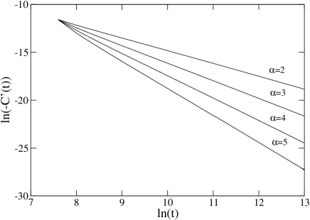
Figure 3: Evolution of the correlation function (123) obtained by solving the Fokker-Planck equation (106) with a logarithmic potential $\Phi(x)=\alpha\ln x$ for $x\geq 1$ and $\Phi(x)=\frac{1}{2}\alpha(x^{2}-1)$ for $x\leq 1$. We have used the boundary condition (108) corresponding to even functions $f(x,t)$. The correlation function is defined by Eqs. (121) and (113) with $A(x)=\ln x$ ($\delta=1$) for $x\geq 1$ and $A(x)=0$ for $x\leq 1$. We have considered different values of $\alpha=2,3,4,5$ (for clarity, the curves have been shifted to the same origin). To get rid of the constant $\langle A\rangle$, we have computed the time derivative $C^{\prime}(t)$ of the correlation function (this is a good strategy otherwise it is not clear whether we should use the exact or the numerical value of $\langle A\rangle$ which differ due to finite resolution). The slope obtained numerically clearly depends on $\alpha$ and is found to be in good agreement with the theoretical prediction (123), up to logarithmic corrections.

Setting $\psi=fe^{\Phi/2}$, we can transform Eq. (106) into a Schrödinger equation with imaginary time

$${\partial{\psi}\over\partial t}={\partial^{2}\psi\over\partial x^{2}}-V_{s}(x)\psi,$$ (114)

with a potential $V_{s}(x)={1\over 4}(\Phi^{\prime})^{2}-{1\over 2}\Phi^{\prime\prime}$. Looking for solutions of the form $\psi\sim e^{-E_{k}t}\psi_{k}(x)$ with $E_{k}=k^{2}$ ($k\geq 0$), we obtain the eigenvalue equation

$$-{d^{2}\psi_{k}\over dx^{2}}+V_{s}(x)\psi_{k}=E_{k}\psi_{k},$$ (115)

with $V_{s}(x)\sim\gamma/x^{2}$ for $x\rightarrow+\infty$ where $\gamma=\alpha(\alpha+2)/4$. Then, the general solution of Eq. (106) with initial condition $f_{A}(x,0)=A(x)f_{e}(x)$ can be written

$$f_{A}(x,t)=e^{-\Phi(x)/2}\left[a_{0}\psi_{0}(x)+\int_{0}^{+\infty}a(k)\psi_{k}(x)e^{-E_{k}t}dk\right].$$

(116)

We assume that the functions $\psi_{k}(x)$ are properly orthonormalized, such that $\int\psi_{k}(x)\psi_{k^{\prime}}(x)dx=\delta(k-k^{\prime})$ and $\int\psi_{0}(x)\psi_{k}(x)dx=\delta_{k,0}$. Taking $t=0$ in Eq. (116), comparing with the initial condition, multiplying by $\psi_{k^{\prime}}(x)$, integrating on $x$ and using the orthonormalization conditions, we obtain after simple calculations

$$a(k)={1\over Z}\int_{0}^{+\infty}A(x)e^{-\Phi(x)/2}\psi_{k}(x)dx,$$ (117)

$$a_{0}={1\over Z}\int_{0}^{+\infty}A(x)e^{-\Phi(x)/2}\psi_{0}(x)dx.$$ (118)

On the other hand, considering the limit $t\rightarrow+\infty$, we find that $\psi_{0}(x)\propto f_{e}(x)e^{\Phi(x)/2}\propto e^{-\Phi(x)/2}$. Therefore, the normalized ground state is

$$\psi_{0}(x)={1\over\sqrt{Z}}e^{-\Phi(x)/2}.$$ (119)

Inserting this expression in Eq. (118), we find that

$$a_{0}={1\over\sqrt{Z}}\int_{0}^{+\infty}A(x)f_{e}(x)dx={1\over\sqrt{Z}}\langle A\rangle.$$ (120)

Inserting Eq. (116) in Eq. (113) and using Eqs. (117) and (120), we finally obtain

$$C(t)\equiv\langle A(0)A(t)\rangle-\langle A\rangle^{2}=Z\int_{0}^{+\infty}a(k)^{2}e^{-E_{k}t}dk.$$

(121)

To obtain the large time behavior of the correlation function, we need to determine the equivalent of $a(k)$ for $k\rightarrow 0$. To that purpose, we need the form of the eigenfunctions $\psi_{k}(x)$ for $k\rightarrow 0$. In the case where $V_{s}(x)\sim\gamma/x^{2}$ for $x\rightarrow+\infty$, corresponding to the logarithmic Fokker-Planck equation, it is possible to solve the eigenvalue equation (115) by match asymptotics mark ; bd and obtain $\psi_{k}(x)$ for $k\rightarrow 0$. Then, we can determine how the correlation function (121) decreases for $t\rightarrow+\infty$ depending on the behavior of the function $A(x)$ for $x\rightarrow+\infty$. Using the results of Marksteiner et al. mark , we find that when $A(x)\sim x^{n}$ the correlation function decreases algebraically like

$$C(t)\sim t^{-\xi},\qquad\xi=-n+{\alpha-1\over 2}.$$ (122)

This result has been given previously by Lutz lutz and Bouchet & Dauxois bd . When $A(x)\sim(\ln x)^{1/\delta}$, using the results of Marksteiner et al. mark , we find that the correlation function decreases like

$$C(t)\sim{(\ln t)^{2/\delta}\over t^{\alpha-1\over 2}}.$$ (123)

This expression has been checked numerically for different values of $\alpha$ (see Fig. 3). For $\alpha=3$, we recover the result $C(t)\sim(\ln t)^{2/\delta}/t$ given by Bouchet & Dauxois bd which turns out to be valid only for this particular value of $\alpha$.

Figure 4: Same as Fig. 3, except that we solve the Fokker-Planck equation with the boundary condition (110) corresponding to odd functions $f(x,t)$. We have considered different values of $\alpha=2,3,4,5,6$. In the present case $\langle A\rangle=0$ so that we can directly plot $C(t)$. The slope obtained numerically clearly depends on $\alpha$ and is found to be in good agreement with the theoretical prediction (123). This is the same value as in Fig. 3 but we note that the scaling regime is reached much more rapidly.

The above results can be easily adapted to the case where the boundary condition is given by Eq. (110) instead of Eq. (108). In that case, $f_{e}(x)$ is not a stationary solution of Eqs. (106)-(110) because it does not satisfy the boundary condition at $r=x=0$. The stationary solution of Eqs. (106)-(110) is $f(x)=0$. This implies that $\psi_{0}(x)=0$ and $a_{0}=0$. As a result, Eq. (121) remains valid provided that we take $\langle A\rangle=0$. Furthermore, since the asymptotic behaviors of Eqs. (122) and (123) obtained from Eq. (121) only depend on the large $x$ behavior of the functions $\psi_{k}(x)$ and not on the boundary condition at $x=0$, these results are valid both for the boundary conditions (110) and (108). This has been checked numerically in Figs. 3 and 4. Interestingly, these numerical simulations show that the scaling regime is reached more rapidly when the boundary condition is given by Eq. (110) instead of Eq. (108).

6 General asymptotic results

We shall now apply the preceding results to the case of point vortices described by the Fokker-Planck equation (68). We first give general results obtained by considering the asymptotic behavior of the diffusion coefficient.

6.1 Asymptotic behavior of the diffusion coefficient

The angular velocity is determined from the vorticity by solving the differential equation

$$\omega={1\over r}{d\over dr}(r^{2}\Omega).$$ (124)

If $\Omega_{1}$ is a particular solution of this equation, the general solution is $\Omega(r)=\Omega_{1}(r)+{C/r^{2}}$ where $C$ is an arbitrary constant. One could a priori consider profiles of angular velocity that are divergent for $r\rightarrow 0$. However, this situation is not physical and in general, the constant $C$ is determined in order to avoid the singularity at $r=0$. In that case, the profile of angular velocity is given by

$$\Omega(r)={1\over r^{2}}\int_{0}^{r}\omega(s)s\;ds.$$ (125)

Asymptotically, we have for $r\rightarrow+\infty$:

$$\Omega(r)\sim{\Gamma\over 2\pi r^{2}},$$ (126)

where $\Gamma$ is the circulation. Then, using Eq. (69), we obtain the asymptotic behavior of the diffusion coefficient

$$D\sim{\pi\gamma\ln\Lambda\over 4\Gamma}r^{2}\omega(r)\propto r^{2}\omega(r).$$ (127)

More generally, combining Eqs. (69) and (124), we find that the diffusion coefficient can be expressed in terms of the angular velocity by

$$D(r)={\gamma\over 4}\ln\Lambda{(r^{2}\Omega)^{\prime}\over|r^{2}\Omega^{\prime}|}.$$ (128)

Alternatively, for a given expression of the diffusion coefficient $D(r)$, the above equation is a first order differential equation for $\Omega(r)$. It can be easily integrated, leading to

$$\Omega(r)={\rm exp}\biggl{\{}-\int{2dr\over[1-{4\epsilon D(r)\over\gamma\ln\Lambda}]r}\biggr{\}},$$ (129)

where $\epsilon=\pm 1$ depending on the sign of the shear ($\epsilon=+1$ if $\Omega^{\prime}>0$ and $\epsilon=-1$ if $\Omega^{\prime}<0$). We note that if $D(r)\rightarrow 0$ for $r\rightarrow+\infty$, which is the situation of physical interest, we get $\Omega(r)\sim{C/r^{2}}$ for $r\rightarrow+\infty$.

6.2 Power law

We first assume that $\omega\propto r^{-\alpha}$ for $r\rightarrow+\infty$. The circulation is finite if $\alpha>2$ and the angular momentum is finite if $\alpha>4$. The diffusion coefficient and the potential behave like

$$D\sim D_{0}r^{-(\alpha-2)},\qquad U(r)\sim\mu\alpha\ln r.$$ (130)

In the following, we shall take $D_{0}=1$ which can always be achieved by rescaling the time appropriately. The stationary solution (97) of the Fokker-Planck equation (96) decreases like $P_{e}\sim r^{-\alpha\mu}$. It is normalizable provided that $\alpha\mu>2$ and the variance $\langle r^{2}\rangle$ is finite provided that $\alpha\mu>4$.

Let us first study the properties of the front structure, using the results of Sec. 5.1. The change of variables $dx/dr=1/\sqrt{D(r)}$ leads to $r\sim(\alpha x/2)^{2/\alpha}$ for $r\rightarrow+\infty$. On the other hand, the velocity field (99) behaves like $V(r)\sim[(2\mu+1)\alpha/2-2]r^{-\alpha/2}$. According to Eq. (100), the position of the front evolves like $r_{f}(t)\sim[\alpha((2\mu+1)\alpha/2-2)t]^{1/\alpha}$. On the other hand, the function defined by Eq. (104) behaves like $g(t)\sim-1/(2t)$ for $t\rightarrow+\infty$. Therefore, according to Eq. (101), we find that the profile of the front characterizing the tail of the distribution for large times is given by

$$u(r,t)\sim\Phi\left[{2\over\alpha}\ {r^{\alpha/2}-\sqrt{\alpha[{(2\mu+1)\alpha\over 2}-2]t}\over(2t)^{1/2}}\right].$$ (131)

For $t\rightarrow+\infty$, the parameter $\epsilon(t)$ controlling the validity of the theory tends to

$$\epsilon={1\over 4}\left({\alpha\over 2}+1\right)\sqrt{4\pi\over\alpha(({2\mu+1})\alpha-4)}.$$ (132)

Since $\epsilon(t)$ does not vanish for $t\rightarrow+\infty$, the theory is only marginally applicable. However, it can still provide a good description of the front structure when $\epsilon$ is sufficiently small cl .

Let us now study the temporal auto-correlation function of the position $\langle r(0)r(t)\rangle$, using the results of Sec. 5.2. The potential defined by Eq. (107) behaves like $\Phi(x)\sim[((2\mu+1)\alpha-4)/\alpha]\ln x$. On the other hand, in terms of the variable $x$, we need to determine the correlation of $A(x)=r(x)\sim x^{2/\alpha}$. According to Eq. (122), we find that

$$\langle r(0)r(t)\rangle-\langle r\rangle^{2}\sim t^{-{(\mu\alpha-4)\over\alpha}}.$$ (133)

6.3 Stretched exponential

We shall now assume that $\omega\sim Ae^{-\lambda r^{\delta}}$ for $r\rightarrow+\infty$. The Gaussian case corresponds to $\delta=2$ and the exponential case to $\delta=1$. The diffusion coefficient and the potential behave like

$$D\sim D_{0}r^{2}e^{-\lambda r^{\delta}},\qquad U(r)\sim\mu\lambda r^{\delta}.$$ (134)

As before, we shall take $D_{0}=1$ without loss of generality. The stationary solution (97) of the Fokker-Planck equation (96) decreases like $P_{e}\sim e^{-\lambda\mu r^{\delta}}$ and all the moments of $r$ are well-defined.

Let us first study the properties of the front structure, using the results of Sec. 5.1. The relation between $x$ and $r$, and the velocity field $V(r)$ are asymptotically given by

$$x\sim{2\over\lambda\delta r^{\delta}}e^{{\lambda\over 2}r^{\delta}},\qquad V(r)\sim{(2\mu+1)\lambda\over 2}\delta r^{\delta}e^{-{\lambda\over 2}r^{\delta}}.$$

(135)

According to Eq. (100), the position of the front evolves like

$${e^{\lambda r_{f}^{\delta}}\over r_{f}^{2\delta}}={(2\mu+1)\lambda^{2}\over 2}\delta^{2}t.$$ (136)

To leading order, we have $r_{f}(t)\sim(\ln t/\lambda)^{1/\delta}$. On the other hand, the function defined by Eq. (104) behaves like $g(t)\sim-1/(2t)$ for $t\rightarrow+\infty$. Therefore, according to Eq. (101), we find that the profile of the front characterizing the tail of the distribution for large times is given by

$$u(r,t)=\Phi\left[{2\over\lambda\delta}{{1\over r^{\delta}}e^{{\lambda\over 2}r^{\delta}}-\sqrt{{(2\mu+1)\lambda^{2}\over 2}\delta^{2}t}\over(2t)^{1/2}}\right].$$ (137)

For $t\rightarrow+\infty$, the parameter $\epsilon(t)$ controlling the validity of the theory tends to

$$\epsilon={1\over 8}\sqrt{4\pi\over 2\mu+1}.$$ (138)

Since $\epsilon(t)$ does not vanish for $t\rightarrow+\infty$, the theory is only marginally applicable. However, we shall see in Sec. 7.1 that the theory still provides a good description of the front structure.

Let us now study the temporal auto-correlation function $\langle r(0)r(t)\rangle$ of the position, using the results of Sec. 5.2. Since $r\sim((2/\lambda)\ln x)^{1/\delta}$, the potential defined by Eq. (107) behaves like $\Phi(x)\sim(2\mu+1)\ln x$. In terms of the variable $x$, we need to determine the correlation of $A(x)=r(x)\sim(\ln x)^{1/\delta}$. Using Eq. (123), we find that

$$\langle r(0)r(t)\rangle-\langle r\rangle^{2}\sim{(\ln t)^{2/\delta}\over t^{\mu}}.$$ (139)

6.4 Behaviour of position-correlations according to the considered vorticity profile

We here qualitatively describe how the position-correlation function decreases depending on the considered vorticity profile. According to Eq. (106), the relaxation towards equilibrium is controlled by the strengh of the drift term $\Phi(x)\sim\alpha_{0}\ln x$, i.e. by the exponent $\alpha_{0}$. Therefore, for large $\alpha_{0}$, the decorrelation should be fast, i.e. $\xi$ should be large, which is indeed the case according to Eqs. (122) and (123). Now, if the vorticity profile decreases like $\omega(r)\sim r^{-\alpha}$, we find that $\alpha_{0}=2\mu+1-4/\alpha$. Therefore, $\alpha_{0}$ is a monotonically increasing function of $\alpha$ tending to $\alpha_{0}=2\mu+1$ for $\alpha\rightarrow+\infty$. On the other hand, the case $\omega(r)\sim e^{-\lambda r^{\delta}}$ leads to $\alpha_{0}=2\mu+1$ which is consistent with the case $\omega(r)\sim r^{-\alpha}$ with $\alpha\rightarrow+\infty$. We conclude therefore that when the vorticity profile decreases rapidly ($\alpha$ large, or stretched exponential), the system decorrelates rapidly ($\alpha_{0}$ large hence $\xi$ large). The physical reason is not simple because the vorticity profile enters both in the diffusion coefficient and in the drift velocity in Eq. (96) so that the decorrelation is a combined effect of these two terms. As discussed above, the situation is more easily interpreted from Eq. (106).

7 Particular examples

In this section, we treat explicit examples corresponding to typical distributions of the field vortices.

7.1 Gaussian vortex

We first consider the case where the distribution of the field vortices corresponds to the statistical equilibrium state (thermal bath). As discussed in Sec. 2, it is obtained by maximizing the entropy of the point vortex gas

$$S=-\int{\omega\over\gamma}\ln{\omega\over\gamma}d{\bf r},$$ (140)

at fixed circulation, energy and angular momentum. This leads to the Boltzmann-Poisson equation

$$\omega=-\Delta\psi=Ae^{-\beta\gamma(\psi+{1\over 2}\Omega_{L}r^{2})}.$$ (141)

This maximization problem provides a condition of thermodynamical stability. According to Appendix A, the functional (140) can also be interpreted as a particular $H$-function (or a Casimir functional). In this sense, a vorticity profile $\omega({\bf r})$ that maximizes $S$ at fixed $\Gamma$, $E$ and $L$ is a nonlinearly dynamically stable stationary solution of the 2D Euler equation. We conclude that for the single species point vortex gas, thermodynamical stability implies nonlinear dynamical stability.

In this section, we consider the case where $\beta\rightarrow 0$ and $\Omega_{L}\rightarrow+\infty$ in such a way that the product $\lambda\equiv\gamma\beta\Omega_{L}/2$ remains finite. The vorticity profile is then given by

$$\omega=\omega_{0}e^{-\lambda r^{2}}.$$ (142)

This will be called the gaussian vortex (note that this is a particular case of Sec. 6.3 with $\delta=2$). The Fokker-Planck equation describing the relaxation of a test vortex in a gaussian bath is

$${\partial P\over\partial t}={1\over r}{\partial\over\partial r}\biggl{[}rD(r)\biggl{(}{\partial P\over\partial r}+2\lambda\mu Pr\biggr{)}\biggr{]}.$$ (143)

The stationary solution is

$$P_{e}(r)={\lambda\mu\over\pi}e^{-\lambda\mu r^{2}}.$$ (144)

It has been normalized such that $\int P_{e}d{\bf r}=1$. Using Eq. (125), the profile of angular velocity of the bath is

$$\Omega={\omega_{0}\over 2\lambda r^{2}}(1-e^{-\lambda r^{2}}).$$ (145)

Therefore, according to Eq. (69), the diffusion coefficient is given by

$$D(r)={D_{0}\lambda r^{2}\over e^{\lambda r^{2}}-\lambda r^{2}-1},$$ (146)

with $D_{0}=(1/4)\gamma\ln\Lambda$ (in the following, we shall take $D_{0}\lambda=1$ by rescaling the time appropriately). We note that the shear vanishes at $r=0$ leading to a divergence of the diffusion coefficient like $D(r)\sim r^{-2}$. This indicates a failure of the kinetic theory for $r\rightarrow 0$. For $r\rightarrow+\infty$, on the other hand, we have $D(r)\propto r^{2}e^{-\lambda r^{2}}$. Since we are particularly interested by the tail of the distribution, we shall extend this expression of the diffusion coefficient for all $r$, thereby circumventing the problems arising for $r\rightarrow 0$ (this regularization shall not change the asymptotic results for $r\rightarrow+\infty$).

Let us first discuss the front structure of the distribution that is solution of the Fokker-Planck equation (143). According to Eq. (136), the evolution of the front position is given by

$${e^{\lambda r_{f}^{2}}\over r_{f}^{4}}=2(2\mu+1)\lambda^{2}t.$$ (147)

For very large times, it can be approximated by $r_{f}(t)\sim(\ln t/\lambda)^{1/2}$ so that the evolution is very slow (logarithmic). On the other hand, according to Eq. (137), the front profile is given by

$$u(r,t)=\Phi\left[{1\over\lambda}{{1\over r^{2}}e^{{\lambda\over 2}r^{2}}-\sqrt{2(2\mu+1)\lambda^{2}t}\over(2t)^{1/2}}\right].$$ (148)

These theoretical results are compared in Figs. 5 and 6 with direct numerical simulations of the Fokker-Planck equation (143). For $\mu=1$, which is the value considered in the numerical simulations, the parameter (138) controlling the validity of the theory is $\epsilon={1\over 8}(4\pi/3)^{1/2}\simeq 0.256...$. Since $\epsilon(t)$ does not tend to zero, the agreement with theory is not perfect, but the relatively small value of $\epsilon$ explains why the theory gives however a fair description of the numerical results. In the present case, we find that the front evolves less rapidly than predicted by the theory (assuming $\epsilon\rightarrow 0$) but this tendency is not general. In cl , we have found other examples where the front evolves more rapidly than predicted by the theory. Understanding this difference requires to develop a theory at order $O(\epsilon)$ in an expansion of the solutions of the front equation in powers of $\epsilon\rightarrow 0$.

Figure 5: Evolution of the front position $r_{f}(t)$ for the Fokker-Planck equation (143) with a diffusion coefficient $D(r)=r^{2}e^{-\lambda r^{2}}$ (we have taken $\mu=\lambda=1$). The details of the procedure are given in cl . The result obtained numerically is in good agreement with the theoretical prediction (147). The agreement is, however, not perfect because the asymptotic value of $\epsilon\simeq 0.256$ is not exactly zero. As a result, the front position (solid line) evolves less rapidly than predicted theoretically (dashed line).

Figure 6: Evolution of the front profile $u(r,t)$ for the Fokker-Planck equation (143) with a diffusion coefficient $D(r)=r^{2}e^{-\lambda r^{2}}$ (we have taken $\mu=\lambda=1$). The solid lines correspond to the numerical simulation and the dashed lines to the theoretical prediction. The initial condition corresponds to the Heaviside function: $P(r,0)=1/(\pi a^{2})$ if $r\leq a$ and $P(r,0)=0$ if $r\geq a$ with $a=2$.

Figure 7: Time evolution of the derivative of the correlation function $C(t)$. It is obtained from Eq. (150) by solving the Fokker-Planck equation (143) with the initial condition $P(r,0)=(1/\pi)re^{-r^{2}}$ (we have taken $\lambda=\mu=1$). For large times, we find that the asymptotic slope of the curve is $2.0704...$, in good agreement with the theoretical value $2$ (up to logarithmic corrections).

Figure 8: This curve suggests that, for large times, the correction to the algebraic decay of the correlation function is logarithmic as expected from the theory.

Finally, according to Eq. (139), the temporal correlation function of the position of the test vortex is predicted to decrease like

$$C(t)\equiv\langle r(0)r(t)\rangle-\langle r\rangle^{2}\sim{\ln t\over t^{\mu}}.$$ (149)

To check this prediction, the function $\langle r(0)r(t)\rangle$ is computed numerically from the expression

$$\langle r(0)r(t)\rangle=\int r_{0}rW({\bf r},t;{\bf r}_{0},0)P_{e}({\bf r}_{0})d{\bf r}_{0}d{\bf r}$$

$$=\int rP_{R}({\bf r},t)d{\bf r},$$ (150)

where $P_{R}({\bf r},t)=P_{R}(r,t)$ is the solution of the Fokker-Planck equation (143) with initial condition $P_{R}({\bf r},0)=rP_{e}({\bf r})$. On the other hand, $\langle r(t)\rangle$ is defined by

$$\langle r(t)\rangle=\int rW({\bf r},t;{\bf r}_{0},0)P_{e}({\bf r}_{0})d{\bf r}_{0}d{\bf r}=\int rP_{E}({\bf r},t)d{\bf r},$$

(151)

where $P_{E}({\bf r},t)=P_{E}(r,t)$ is the solution of the Fokker-Planck equation (143) with initial condition $P_{E}({\bf r},0)=P_{e}({\bf r})$. Since $P_{E}({\bf r},t)=P_{e}({\bf r})$ for all times (this is the stationary solution), we find that $\langle r(t)\rangle=\langle r\rangle$ is the average of $r$ with the equilibrium distribution (144). Thus, $\langle r\rangle={1\over 2}(\pi/\lambda\mu)^{1/2}$. We also note that $\int P_{R}d{\bf r}=\langle r\rangle$ so that $P_{R}(r,+\infty)=\langle r\rangle P_{e}(r)$. Therefore, according to Eq. (150), $\langle r(0)r(t)\rangle\rightarrow\langle r\rangle^{2}$ for $t\rightarrow+\infty$. This is why we need to subtract the term $\langle r\rangle^{2}$ in the correlation function (149). To avoid numerical errors in the evaluation of $\langle r\rangle$ (due to finite resolution), we have chosen to study the derivative of the correlation function which is predicted to behave like

$$C^{\prime}(t)\sim-{\ln t\over t^{\mu+1}}.$$ (152)

The results of the numerical simulations are represented in Figs. 7 and 8. Figure 7 shows that the correlation function decays algebraically with the correct exponent predicted by the theory (up to logarithmic corrections considered in Fig. 8).

In conclusion, we find that the relaxation of the distribution function $P(r,t)$ to the equilibrium state (144) is peculiar. The evolution of the front position is very slow (logarithmic) and the temporal correlation function decreases algebraically (up to logarithmic corrections). These results differ from the traditional exponential relaxation in the usual Brownian theory. They are due to the rapid (gaussian) decrease of the diffusion coefficient with $r$. The same behaviours have been found for the HMF model bd ; cl .

7.2 Isothermal vortex in a disk

We now consider the case of an isothermal vortex (141) in a disk of radius $R$ and assume that $\Omega_{L}=0$. This corresponds to a particular value of the angular momentum $L_{0}(E,\Gamma)$ for a given energy $E$ and circulation $\Gamma$. The equilibrium profile is then determined by solving the Boltzmann-Poisson equation

$$-{1\over r}{d\over dr}\left(r{d\psi\over dr}\right)=Ae^{-\beta\gamma\psi}=\omega_{0}e^{-\beta\gamma(\psi-\psi_{0})},$$ (153)

with $\psi^{\prime}(0)=0$ and $\psi(R)=0$. This equation can be solved analytically, see e.g. caglioti ; houches . The vorticity profile is explicitly given by

$$\omega={4\Gamma\over\pi R^{2}(\eta+4)}{1\over\bigl{(}1-{\eta\over\eta+4}{r^{2}\over R^{2}}\bigr{)}^{2}},$$ (154)

where $\eta=\beta\gamma\Gamma/(2\pi)$ is a normalized temperature. From this distribution, we can determine the mean field energy. The caloric curve $\beta(E)$ is given in houches . There exists solutions for any value of the normalized energy $\epsilon=2\pi E/(N^{2}\Gamma^{2})\geq 0$. The corresponding temperature satisfies $\eta>\eta_{c}=-4$, i.e. $\beta>\beta_{c}=-8\pi/(\gamma\Gamma)$. For $\beta>0$, the vorticity increases with the distance and for $\beta<0$, the vorticity decreases with the distance. For $\beta=\beta_{c}$, we have $\omega({\bf r})=\Gamma\delta({\bf r})$ so that $\epsilon\rightarrow+\infty$. Typical vorticity profiles are shown in houches depending on the value of the temperature.

The Fokker-Planck equation describing the motion of a test vortex in a thermal bath specified by the distribution (154) is

$${\partial P\over\partial t}={1\over r}{\partial\over\partial r}\biggl{[}rD(r)\biggl{(}{\partial P\over\partial r}-{4\mu P\eta r\over(\eta+4)R^{2}-\eta r^{2}}\biggr{)}\biggr{]}.$$ (155)

The profile of angular velocity corresponding to the isothermal vortex (154) is

$$\Omega=-{2\Gamma\over\pi R^{2}(\eta+4)}{1\over 1-{\eta\over\eta+4}{r^{2}\over R^{2}}}.$$ (156)

Therefore, according to Eq. (69), the diffusion coefficient is given by

$$D(r)={\gamma\over 4}\ln\Lambda{\eta+4\over|\eta|}{R^{2}\over r^{2}}.$$ (157)

Again, this expression is valid only for $r\gg 1$. Setting $x=(1/2)(r/R)^{2}$, $C=-\eta/(\eta+4)$, $D_{0}={\gamma}\ln\Lambda{(\eta+4)/|\eta|}$ and $\tau=D_{0}t/4R^{2}$, we can rewrite the Fokker-Planck equation as

$${\partial P\over\partial\tau}={\partial\over\partial x}\biggl{(}{\partial P\over\partial x}+{\Gamma_{0}\over\gamma}{4CP\over 1+2Cx}\biggr{)},$$ (158)

with $0\leq x\leq 1$. This is of the form of Eq. (106) with a logarithmic potential $\Phi(x)=2\mu\ln(1+2Cx)$. With the change of variable $\psi=Pe^{\Phi/2}=(1+2Cx)^{\mu}P$, it can be transformed into a Schrödinger equation with imaginary time

$${\partial{\psi}\over\partial\tau}={\partial^{2}\psi\over\partial x^{2}}-V_{s}(x)\psi,$$ (159)

with a potential

$$V_{s}(x)={\lambda C^{2}\over(1+Cx)^{2}},$$ (160)

where $\lambda=4\mu(1+\mu)$. Since the domain is bounded, we cannot apply the results of Secs. 5.1 and 5.2 which assume that the tail of the distribution extends to infinity. Therefore, in the next section, we shall consider the isothermal vortex in an unbounded domain.

7.3 Isothermal vortex in an infinite domain

In an infinite domain, extending the calculations of houches , we find that the Boltzmann-Poisson equation (153) has solution only for the critical temperature

$$\beta_{c}=-\frac{8\pi}{\gamma\Gamma},$$ (161)

and that the vorticity profile is given by the family of solutions

$$\omega(r)={\omega_{0}\over(1+{\pi\omega_{0}\over\Gamma}r^{2})^{2}},$$ (162)

parameterized by the central vorticity $\omega_{0}$. Since $\omega\sim r^{-4}$ at large distances, we note that the angular momentum diverges logarithmically. From the Poisson equation (7) with the vorticity field (162), we find that the streamfunction is given by

$$\psi(r)=-{\Gamma\over 4\pi}\ln\left(\frac{\Gamma}{\pi\omega_{0}}+r^{2}\right),$$ (163)

where we have assumed that $\psi+{\Gamma\over 2\pi}\ln r\rightarrow 0$ for $r\rightarrow+\infty$ in order to determine the Gauge constant. The energy of interaction $E={1\over 2}\int\omega\psi d{\bf r}$ is finite and its value is

$$E=-{\Gamma^{2}\over 8\pi}+{\Gamma^{2}\over 8\pi}\ln\left({\pi\omega_{0}\over\Gamma}\right).$$ (164)

This relation determines the central density $\omega_{0}$ as a function of $E$. The caloric curve is a straight line with constant temperature $\beta=\beta_{c}$ for all energies. We note that the kinetic energy $E^{\prime}={1\over 2}\int{\bf u}^{2}d{\bf r}={1\over 2}\int(\nabla\psi)^{2}d{\bf r}$ diverges logarithmically. It differs from the energy of interaction $E$ because the boundary terms do not vanish in the present case.

The Fokker-Planck equation describing the relaxation of a test vortex in a thermal bath specified by the distribution (162) is

$${\partial P\over\partial t}={1\over r}{\partial\over\partial r}\left[rD(r)\left({\partial P\over\partial r}+{4\mu Pr\over{\Gamma\over\pi\omega_{0}}+r^{2}}\right)\right].$$ (165)

The profile of angular velocity corresponding to the isothermal vortex (162) is given by

$$\Omega(r)={\omega_{0}\over 2\left(1+{\pi\omega_{0}\over\Gamma}r^{2}\right)}.$$ (166)

Therefore, the diffusion coefficient is

$$D(r)={\gamma\Gamma\over 4\pi\omega_{0}}\ln\Lambda{1\over r^{2}}.$$ (167)

Setting $x=(\pi\omega_{0}/2\Gamma)r^{2}$, $D_{0}=\pi\gamma\ln\Lambda$ and $\tau=D_{0}\omega_{0}t/4\Gamma$, the Fokker-Planck equation can be rewritten

$${\partial P\over\partial\tau}={\partial\over\partial x}\left({\partial P\over\partial x}+{4\mu P\over 1+2x}\right),$$ (168)

with $x\in[0,\infty[$. This is of the form of Eq. (106) with a logarithmic potential $\Phi(x)=2\mu\ln(1+2x)$. With the change of variable $\psi=Pe^{\Phi/2}=(1+2x)^{\mu}P$, it can be transformed into a Schrödinger equation of the form (159) with a potential

$$V_{s}(x)={\lambda\over(1+2x)^{2}},$$ (169)

where $\lambda=4\mu(1+\mu)$. In the following, we set $(\gamma\Gamma/4\pi\omega_{0})\ln\Lambda=1$ and $\Gamma/\pi\omega_{0}=1$ which can always be achieved by rescaling the time and the distances appropriately. Then, the results of Sec. 5 can be directly applied with $\alpha=4$. Concerning the tail of the distribution, the position of the front is given by

$$r_{f}(t)\sim(16\mu t)^{1/4},$$ (170)

and the profile of the front is

$$u(r,t)\sim\Phi\left[2\ {r^{2}-\sqrt{16\mu t}\over(2t)^{1/2}}\right].$$ (171)

As discussed in Sec. 5.1, the theory is only marginally applicable. However, it can give a fair description of the front if the parameter $\epsilon=(3/8)\sqrt{\pi/2\mu}$ is sufficiently small (for $\mu=1$, we have $\epsilon\simeq 0.47$). On the other hand, the temporal correlation function decreases like

$$\langle r(0)r(t)\rangle-\langle r\rangle^{2}\sim t^{-(\mu-1)}.$$ (172)

We note that we must impose $\mu>1$ otherwise the variance $\langle r^{2}\rangle$ of the equilibrium state diverges.

7.4 Polytropic vortex

As discussed in Sec. 3, the distribution of the bath can be any stable stationary solution of the 2D Euler equation with a monotonic profile of angular velocity, not necessarily the statistical equilibrium state. A general criterion of nonlinear dynamical stability is given in Appendix A. As an explicit example, let us consider an $H$-function (or Casimir integral) of the form

$$S_{q}=-{1\over q-1}\int(\omega^{q}-\omega)d{\bf r}.$$ (173)

A vorticity distribution which maximizes this functional at fixed circulation and energy (and angular momentum) is nonlinearly dynamically stable with respect to the 2D Euler equation. The variational problem (191) leads to a relationship between the vorticity and the stream function of the form

$$\omega=\left[\mu-{\beta(q-1)\over q}\psi^{\prime}\right]^{1\over q-1}.$$ (174)

We shall call these vortices polytropic vortices gen because they are analogous to stellar polytropes in astrophysics bt . The structure and the stability of stellar polytropes in $d$ dimensions has been studied in lang . For $d=2$, we can easily adapt these results to describe polytropic vortices. Note that the functional (173) and the corresponding distribution (174) are similar to the so-called Tsallis entropies and Tsallis distributions introduced in non-standard thermodynamics tsallis . However, in the present context, they have a completely different interpretation [63,66-69]. They correspond to dynamical, not thermodynamical, equilibrium states. In particular, the maximization of $S_{q}$ at fixed circulation and energy is a condition of nonlinear dynamical stability for the 2D Euler-Poisson system, not a condition of generalized thermodynamical stability. The distributions (174) form just a particular family of stationary solutions of the 2D Euler equation that can sometimes give a good fit of the quasi-stationary state (QSS) resulting from an incomplete violent relaxation jfm2 ; brands ; fermiHMF . This dynamical interpretation of the functional (173) is different from the interpretation given by Boghosian boghosian in terms of Tsallis generalized thermodynamics. For $q\rightarrow 1$, we recover the isothermal vortex (141) as a special case. For $q=2$, we have

$$S_{2}=-\int\omega^{2}d{\bf r},$$ (175)

up to an additive constant. Therefore, the neg-enstrophy $S_{2}=-\Gamma_{2}$ can be interpreted as a particular $H$-function (or Casimir integral). In that case, the relationship (174) is linear

$$\omega=\mu-{1\over 2}\beta\psi^{\prime}.$$ (176)

The structure and the stability of these linear vortices has been studied in detail in jfm1 ; jfm2 . In these studies, the enstrophy was interpreted as an approximation of the Miller-Robert-Sommeria mixing entropy [47-50] in a limit of strong mixing (or low energy). Therefore, the results of jfm1 ; jfm2 were presented as results of thermodynamical stability for the process of violent relaxation (in a particular limit of the theory). Alternatively, if we view the enstrophy as an $H$-function (see Appendix A), the results of jfm1 ; jfm2 can also be interpreted as results of nonlinear dynamical stability with respect to the 2D Euler equation.

For illustration, let us consider the case of a disk of radius $R$ and take $\Omega_{L}=0$. We also assume that the vortex fills the whole domain and that $\omega(R)=\psi(R)=0$. This implies that $\mu=0$ in Eq. (176). We then obtain the Helmholtz equation

$$\Delta\psi+k^{2}\psi=0,$$ (177)

where $k^{2}=-\beta/2$ (we have assumed $\beta<0$). The solution is $\psi=AJ_{0}(\alpha r/R)$ where $\alpha=kR=2.40482...$ is the first zero of the Bessel function $J_{0}(x)$. Setting $\omega_{0}=\alpha^{2}A/R^{2}$, the vorticity profile is

$$\omega=\omega_{0}J_{0}(\alpha r/R).$$ (178)

The Fokker-Planck equation describing the relaxation of a test vortex in a bath specified by the distribution (178) is

$${\partial P\over\partial t}={1\over r}{\partial\over\partial r}\left[rD(r)\left({\partial P\over\partial r}+{\alpha\Gamma_{0}\over\gamma R}P{J_{1}(\alpha r/R)\over J_{0}(\alpha r/R)}\right)\right].\qquad$$ (179)

Using $(xJ_{1})^{\prime}=xJ_{0}$, the profile of angular velocity corresponding to the Bessel distribution (178) is given by

$$\Omega={R\omega_{0}\over\alpha r}J_{1}(\alpha r/R).$$ (180)

Therefore, according to Eq. (69), the diffusion coefficient can be written

$$D(r)={\gamma\over 4}\ln\Lambda{{\alpha r\over R}J_{0}(\alpha r/R)\over 2J_{1}(\alpha r/R)-{\alpha r\over R}J_{0}(\alpha r/R)}.$$ (181)

Considering now the limit $\beta\rightarrow 0$ and $\Omega_{L}\rightarrow+\infty$ in such a way that the product $\lambda=\beta\Omega_{L}/2$ remains finite, we obtain

$$\omega(r)=\left[1-{\lambda(q-1)\over q}r^{2}\right]^{1\over q-1}.$$ (182)

For $q\rightarrow 1$, we recover the gaussian vortex (142). For $q>1$, the vorticity vanishes at a finite radius $R_{*}$ (we take $\omega=0$ for $r>R_{*}$). For $q<1$, the vorticity decreases like $\omega\sim r^{-2/(1-q)}$. This algebraic behavior falls in the class of solutions studied in Sec. 6.2.

7.5 Fermi-Dirac vortex

As a last example, we consider a typical prediction of the statistical mechanics of violent relaxation of the 2D Euler equation [47-50]. In the two-levels approximation, the statistical equilibrium state is obtained by maximizing the mixing entropy

$$S=-\int\left\{{\overline{\omega}\over\sigma_{0}}\ln{\overline{\omega}\over\sigma_{0}}+\left(1-{\overline{\omega}\over\sigma_{0}}\right)\ln\left(1-{\overline{\omega}\over\sigma_{0}}\right)\right\}d{\bf r},\qquad$$ (183)

at fixed circulation, energy and angular momentum. This leads to a distribution of the form

$$\overline{\omega}={\sigma_{0}\over 1+Ke^{\beta\psi^{\prime}}},$$ (184)

with $K>0$. This will be called the Fermi-Dirac vortex. This distribution of the bath can emerge from a complete violent relaxation of the 2D Euler-Poisson system in the first regime of the dynamics (see discussion in the Conclusion). According to Appendix A, a maximum of the entropy (183) at fixed energy and circulation (thermodynamical equilibrium state in the theory of violent relaxation) is nonlinearly dynamically stable with respect to the 2D Euler-Poisson system. For $K\rightarrow+\infty$, we recover the isothermal vortex (141) and for $K\rightarrow 0$, we obtain a vortex with uniform vorticity surrounded by irrotational flow (this is the analogous of the Fermi distribution in phase space). Considering now the limit $\beta\rightarrow 0$ and $\Omega_{L}\rightarrow+\infty$ in such a way that the product $\lambda=\beta\Omega_{L}/2$ remains finite, we obtain

$$\overline{\omega}={\sigma_{0}\over 1+Ke^{\lambda r^{2}}}.$$ (185)

For $K\rightarrow+\infty$, we recover the gaussian vortex (142). More generally, the bath distribution behaves like $\overline{\omega}\sim e^{-\lambda r^{2}}$ for $r\rightarrow+\infty$ so that the results of Sec. 7.1 apply to the present context.

8 Conclusion

In this paper, we have developed the kinetic theory of point vortices in two-dimensional hydrodynamics. The interest of this kinetic theory goes beyond the realm of fluid mechanics since the point vortex gas constitutes a system of particles with long-range interactions (like self-gravitating systems) which displays peculiar features in regard to statistical mechanics and kinetic theory houches . Starting from the Liouville equation and using the projection operator formalism, we have derived a kinetic equation (29) that describes the evolution of the system as a whole. This kinetic equation conserves all the constraints of the point vortex dynamics (circulation $\dot{\Gamma}=0$, energy $\dot{E}=0$ and angular momentum $\dot{L}=0$) and increases the Boltzmann entropy monotonically ($\dot{S}\geq 0$). However, it does not necessarily relax towards the Boltzmann distribution of statistical equilibrium because this kinetic equation admits an infinite number of stationary solutions and the evolution stops when there is no resonance anymore (this happens when the profile of angular velocity becomes monotonic). In that case, the vorticity profile can remain frozen in a QSS with a non-Boltzmannian distribution until more complex (e.g., three body) correlations come into play. This has been shown numerically in Sec. 3.4. We have next considered the relaxation of a test vortex in a steady bath of field vortices. This relaxation is described by a Fokker-Planck equation (60) with a space dependent diffusion coefficient. We have studied analytically and numerically some properties of this Fokker-Planck equation regarding the evolution of the front profile in the tail of the distribution function and the decay of the temporal correlation function of the position of the test vortex depending on the distribution of the bath. For a thermal bath (gaussian vortex), we have shown that the evolution of the front position is logarithmic, scaling like $r_{f}(t)\propto(\ln t)^{1/2}$ and that the temporal correlation function of the position decreases algebraically (up to logarithmic corrections), scaling like $\langle\Delta r(0)\Delta r(t)\rangle\propto\ln t/t$. This is at variance with the exponential decay of correlations for the usual Brownian motion (with constant diffusion coefficient and linear drift) but this is similar with results obtained for the HMF model bd ; cl . We would like to conclude this paper by discussing the different regimes that take place in the dynamics of point vortices. This discussion is important to clarify certain points in order to answer some of the criticisms raised by Dubin dubin and discuss specifically the domains of application of the different kinetic theories.

Basically, a system of point vortices is described by the $N$-body Hamiltonian equations of motion (1)-(2). From these equations, we can derive the Klimontovich equation for the exact vorticity field $\omega_{exact}({\bf r},t)=\sum_{i}\gamma_{i}\delta({\bf r}-{\bf r}_{i}(t))$ expressed in terms of $\delta$-functions (see Eq. (15) of kin ) or the Liouville equation for the $N$-body distribution $P_{N}({\bf r}_{1},...,{\bf r}_{N},t)$ (see Eq. (59) of kin ). These exact equations are equivalent to the $N$-body dynamics and contain too much information to be of practical use. The object of the kinetic theory is to derive an equation for the smooth vorticity field $\omega({\bf r},t)=\langle\sum_{i}\gamma_{i}\delta({\bf r}-{\bf r}_{i}(t))\rangle$ or the one-body distribution $P_{1}({\bf r},t)$ (see Sec. 3.1). By rescaling the variables appropriately, we have seen that the “collision term” could be evaluated in an expansion in powers of $1/N$ for $N\rightarrow+\infty$ with fixed normalized energy $\epsilon=E/(N^{2}\gamma^{2})$ and fixed normalized temperature $\eta=\beta\gamma\Gamma$. This unusual thermodynamic limit corresponds to $N\rightarrow+\infty$ with $\gamma\sim 1/N$ and $V\sim 1$ (implying $E\sim 1$ and $\beta\sim N$). For the moment, only the term of order $O(1/N)$ in the kinetic theory has been computed [see Eq. (14)]. This amounts to neglecting three-body (or higher) correlations among the vortices. These points are made clear in bbgky .

To leading order in $N\rightarrow+\infty$, the evolution of the smooth vorticity field $\omega({\bf r},t)$ representing the spatial distribution of the point vortices is governed by the 2D Euler-Poisson system (see Eq. (125) of kin ) as for inviscid and incompressible 2D flows with continuous vorticity. This Vlasov (or mean field) limit amounts to neglecting all the correlations among the vortices. Physically, this regime is valid for $t\ll Nt_{D}$ and its domain of validity can be very long when $N$ is large. The 2D Euler-Poisson system has a very complex dynamics. Starting from an unstable initial condition $\omega_{0}({\bf r})$, the 2D Euler-Poisson system develops a complicated mixing process leading ultimately to a Quasi Stationary State (QSS), also called a metaequilibrium state, which has the form of a vortex or a jet. This “collisionless relaxation” is similar to the process of violent relaxation in astrophysics based on the Vlasov-Poisson system lb ; csr ; houches . It takes place on a timescale of the order of a few dynamical times $t_{D}$. The resulting QSS is a stable stationary solution of the 2D Euler equation on the coarse-grained scale $\overline{\omega}({\bf r})$, i.e. if we locally average over the filaments. A statistical theory has been developed by Miller miller and Robert & Sommeria rs in order to predict the most probable equilibrium state resulting from a violent relaxation. This theory is based on a hypothesis of ergodicity, assuming that the relaxation is complete, so that the system is expected to be in the most mixed state. This is similar to the statistical theory of Lynden-Bell lb for collisionless stellar systems. A kinetic theory of the process of violent relaxation has been proposed by Robert & Sommeria rsmep , and further developed in csr ; rr ; csprl , by using a phenomenological Maximum Entropy Production Principle (MEPP). They obtained a drift-diffusion equation for the coarse-grained vorticity $\overline{\omega}({\bf r},t)$ with a time dependent temperature $\beta(t)$ that evolves in order to satisfy the conservation of energy (see Eqs. (11)-(12) of rsmep ). In order to determine the domain of validity of this phenomenological approach and determine the value of the diffusion coefficient (which is not given by the MEPP), Chavanis prl attempted to develop a kinetic theory of violent relaxation, starting directly from the 2D Euler equation and using a systematic procedure based on a coarse-graining and a linearization of the equation for the fluctuations. This quasilinear theory was developed in analogy with the quasilinear theory of the Vlasov-Poisson system in astrophysics kp ; sl . The approach of Chavanis prl remains, however, unsatisfactory because it yields an equation [see Eq. (20)] which does not conserve energy. This could be cured as proposed in kin [see Eq. (148)] by taking into account resonances between the motion of the fluid particles but this procedure may not be completely justified since there is no real timescale separation between the decrease of correlations and the evolution of the coarse-grained vorticity field (unlike during the slow collisional relaxation of point vortices). As a result, memory (non-Markovian) effects are expected to be important in the process of violent relaxation. Note that the more general equation (18) derived in prl may conserve energy and provide a correct description of the coarse-grained dynamics bbgky .

If we now consider an axisymmetric distribution of point vortices that is stable with respect to the 2D Euler equation and if we take into account terms of order $1/N$ in the kinetic theory, we describe the “collisional” relaxation process. The kinetic equation governing the evolution of the system as a whole is given by Eq. (29) obtained by Chavanis kin , or by the more general kinetic equation taking into account collective effects obtained by Dubin & O’Neil dn . Physically, this regime is valid on a timescale $Nt_{D}$. For single species systems, the evolution of the smooth vorticity field is due to a condition of resonance $\Omega(r,t)=\Omega(r^{\prime},t)$ which can be satisfied only when the profile of angular velocity is non-monotonic. As a result, the evolution stops when the profile of angular velocity becomes monotonic so that there is no resonance anymore. In that case, the system remains frozen in a long-lived QSS. This is a stationary solution of the 2D Euler equation which usually differs from the statistical equilibrium state (Boltzmann distribution) predicted by Joyce & Montgomery jm and Lundgren & Pointin lp . The fact that the system can be frozen in a QSS state in the absence of resonance was stressed in kin . This implies either that the system will not reach statistical equilibrium at all or that the kinetic theory is incomplete. Indeed, the collision term calculated in the kinetic theory of Dubin & O’Neil dn and Chavanis kin corresponds to a term of order $1/N$ in a systematic expansion carried out in a proper thermodynamic limit $N\rightarrow+\infty$. In particular, it neglects non-trivial three-body correlations. Therefore, this theory describes the dynamics of the system on a timescale of order $Nt_{D}$ where $t_{D}$ is the dynamical time. If the collision term cancels out because of the absence of resonance, i.e. when the profile of angular velocity becomes monotonic, the relaxation towards statistical equilibrium (if any) will take place on a timescale larger than $Nt_{D}$ so that next order terms in the $1/N$ expansion must be taken into account in the kinetic theory. These higher order terms have not yet been considered. Therefore, there is no certitude, up to date, that the point vortex gas relaxes towards statistical equilibrium for $t\rightarrow+\infty$. This could be checked in numerical simulations of the point vortex dynamics by solving the Hamilton equations (1)-(2). A challenging problem is to determine the collisional relaxation time $t_{relax}$ of the point vortex gas towards statistical equilibrium. According to the present kinetic theory it should scale like $t_{relax}\sim N^{\delta}t_{D}$ with $\delta\geq 1$ but the precise value of $\delta$ is not yet known (see Sec. 4.4). In numerical simulations, we must be careful not to confound the true statistical equilibrium state resulting from a slow collisional relaxation for large times (larger that $Nt_{D}$) with the QSS resulting from a violent collisionless relaxation taking place on a much shorter timescale $\sim t_{D}$. Indeed, there are many confusions in the literature between the Joyce-Montgomery jm statistical equilibrium state (collisional relaxation) and the Miller-Robert-Sommeria miller ; rs statistical equilibrium state (collisionless relaxation). Although these statistical distributions are mathematically similar in certain limits (dilute limit), their physical origin is completely different since they apply to different regimes of the point vortex dynamics. This implies in particular that the two theories are not in conflict since they refer to completely different regimes.

Finally, if we consider the relaxation of a test particle in a thermal bath of point vortices at statistical equilibrium, we obtain a Fokker-Planck equation (73) which has the form of a drift-diffusion equation with a space dependent diffusion coefficient inversely proportional to the local shear created by the bath. This Fokker-Planck equation derived by Chavanis preR ; kin is similar to the relaxation equation proposed phenomenologically by Robert & Sommeria rsmep by using the MEPP to describe the evolution of the 2D Euler equation on the coarse-grained scale during the process of violent relaxation. However, this resemblance is essentially coincidental since the two theories describe completely different situations and different timescales. Therefore, the kinetic theory of point vortices is rich and different regimes can be evidenced. For that reason, it is important to delimit the domains of application of each kinetic theory in order to avoid misunderstandings. Indeed, the mathematical structure of the kinetic equations can be formally similar while describing completely different situations. When the conditions of validity of the different theories are properly delineated, there are no contradiction between our results and those obtained by Dubin dubin . The works are complementary.

In future works, it will be important to evaluate terms of higher order in the development in $1/N$ of the kinetic equation so as to describe the evolution of the system on longer timescales. This implies the evaluation of two and three-body correlation functions, which is a formidable task. We must also distinguish the case where the circulations of the point vortices have the same sign or a different sign. When the circulations of the point vortices take positive and negative values, the point vortices can group themselves in dipoles or tripoles. As indicated in Sec. 2, this situation cannot be described by the mean field theory. The system will then have a very different dynamics than the one described here (in Sec. 3.2). For example, Sire & Chavanis sc show that the merging between vortices in 2D decaying turbulence is due essentially to collisions between dipoles and monopoles. The inclusion of dipoles and tripoles in the kinetic theory needs to take into account two and three-body correlation functions as discussed by Newton & Mezic nm . In our approach, these pairs would form on a timescale larger than $Nt_{D}$ so they have not been taken into account. We note, finally, that our approach implicitly assumes that there are no correlations initially so that the $1/N$ development is well-defined (see bbgky for more details). If pairs $(+,+)$, dipoles $(+,-)$, tripoles $(+,-,+)$ or more complex “structures” exist initially, then we must take into account high order correlations since the start and the kinetic theory will be different.

Another extension of the kinetic theory is to consider flows that are not axisymmetric. In that case, the kinetic equation valid at the order $1/N$ is given by Eq. (14). It describes the evolution of the system as a whole on a timescale $Nt_{D}$. Using the timescale separation between the dynamical time $t_{D}$ and the collisional relaxation time $t_{relax}$ (of order $Nt_{D}$ or larger), it would be of interest to derive an “orbit-averaged” kinetic equation in terms of appropriate variables similar to the angle-action variables used in other contexts bt ; action . The resulting kinetic equation would be more complicated than Eq. (29) but the basic concepts remain the same. For non-axisymmetric flows, we can have a lot of resonances (see the expectedly similar case in action ) and they can “push” the system towards a distribution close to the Boltzmann distribution on a timescale $\sim Nt_{D}$ (the exact Boltzmann distribution should be reached however on longer timescales due to higher order terms $1/N^{2}$, $1/N^{3}$,… in the kinetic equation). The same remark applies to the inhomogeneous phase of the HMF model as discussed in action . While there is no evolution at all on a timescale $Nt_{D}$ in the homogeneous phase of the HMF model (because there is no resonance), many resonances appear in the inhomogeneous phase which can “push” the system towards a distribution close to the Boltzmann distribution on a timescale $Nt_{D}$. These interesting problems should be given further consideration in future works.

Appendix A Nonlinear dynamical stability of stationary solutions of the 2D Euler equation

We consider the 2D Euler-Poisson system

$${\partial\omega\over\partial t}+{\bf u}\cdot\nabla\omega=0,\qquad{\bf u}=-{\bf z}\times\nabla\psi,\qquad\omega=-\Delta\psi.$$

(186)

Any relation of the form $\omega=f(\psi)$ determines a stationary solution of the 2D Euler equation $\partial\omega/\partial t=0$ since $\nabla\omega=f^{\prime}(\psi)\nabla\psi$ is perpendicular to ${\bf u}$. This result is valid in an arbitrary domain. In a disk or in an infinite domain, we can also consider pseudo-stationary solutions of the form $\omega(r,\theta,t)=\omega(r,\theta-\Omega_{L}t)$ that describe a structure rotating uniformly with angular velocity $\Omega_{L}$ (the system is stationary in the rotating frame). If we write the 2D Euler equation in the form

$${\partial\omega\over\partial t}+{1\over r}{\partial\psi\over\partial\theta}{\partial\omega\over\partial r}-{1\over r}{\partial\psi\over\partial r}{\partial\omega\over\partial\theta}=0,$$ (187)

and substitute for the preceding relation, we find that

$${\partial\psi\over\partial\theta}{\partial\omega\over\partial r}-\left(\Omega_{L}r+{\partial\psi\over\partial r}\right){\partial\omega\over\partial\theta}=0.$$ (188)

This equation is satisfied by any relation of the form $\omega=f(\psi^{\prime})$ where $\psi^{\prime}=\psi+{1\over 2}\Omega_{L}r^{2}$ is the relative streamfunction.

One important question concerns the dynamical stability of a stationary solution of the 2D Euler equation. Let us introduce the functionals

$$S=-\int C(\omega)d{\bf r},$$ (189)

where $C$ is any convex function, i.e. $C^{\prime\prime}>0$. Such functionals form a particular class of Casimirs. They are also called generalized $H$-functions for the reasons explained in tremaine ; physicaA . It can be shown that the maximization problem

$${\rm Max}\{S[\omega]\quad|\quad E[\omega]=E,\Gamma[\omega]=\Gamma,L[\omega]=L\},$$ (190)

determines a steady solution of the 2D Euler equation with monotonic $\omega=f(\psi^{\prime})$ relationship that is nonlinearly dynamically stable . This condition of nonlinear dynamical stability has been proven by Ellis et al. ellis . It refines the Arnold’s sufficient criteria of nonlinear dynamical stability and solves some apparent “paradoxes” observed in geophysical fluid dynamics (some flows can be dynamically stable according to the criterion (190) although they do not satisfy the Arnold criteria) ellis ; physicaD . Note that the nonlinear dynamical stability criterion (190) has been proven in the absence of angular momentum constraint. When the angular momentum is conserved, the optimization problem (190) determines a family of solutions that can be deduced from each other by a mere rotation. In that case, the notion of nonlinear dynamical stability must be reconsidered to account for this property.

Introducing Lagrange multipliers and writing the first order variations as

$$\delta S-\beta\delta E-{1\over 2}\beta\Omega_{L}\delta L-\alpha\delta\Gamma=0,$$ (191)

we get

$$C^{\prime}(\omega)=-\beta\psi^{\prime}-\alpha,$$ (192)

where $\psi^{\prime}$ is the relative stream function defined above. Since $C$ is monotonic, this relation can be reversed to give $\omega=F(\beta\psi^{\prime}+\alpha)=f(\psi^{\prime})$ where $F(x)=(C^{\prime})^{-1}(-x)$. Therefore $f$ is monotonic. It is increasing at negative “temperatures” and decreasing at positive “temperatures”, since $\omega^{\prime}(\psi^{\prime})=-\beta/C^{\prime\prime}(\omega)$. When $\beta\rightarrow 0$ and $\Omega_{L}\rightarrow+\infty$ in such a way that the product $\lambda\equiv{1\over 2}\beta\Omega_{L}$ remains finite, the previous solution becomes $\omega=F(\lambda r^{2}+\alpha)$.

In conclusion, the critical points of the optimization problem (190) determine steady states of the 2D Euler equation (in a rotating frame). Furthermore, maxima of $S$ at fixed $E$, $\Gamma$ (and $L$) are nonlinearly dynamically stable.

Appendix B The calculation of the function $M$

The velocity (by unit of circulation) created by point vortex $1$ located in ${\bf r}_{1}$ on point vortex $0$ located in ${\bf r}$ is

$${\bf V}(1\rightarrow 0)={1\over 2\pi}\hat{\bf z}\times{{\bf r}-{\bf r}_{1}\over|{\bf r}-{\bf r}_{1}|^{2}}={1\over 2\pi}\hat{\bf z}\times\nabla\ln|{\bf r}-{\bf r}_{1}|.$$

(193)

Therefore, the radial component $V_{r}={\bf V}\cdot\hat{\bf r}$ of the velocity in the direction of the test vortex $0$ can be written

$$V_{r}(1\rightarrow 0)=-{1\over 2\pi r}{\partial\over\partial\theta}\ln|{\bf r}-{\bf r}_{1}|.$$ (194)

Introducing a polar system of coordinates $(r,\theta)$ to localize a point vortex and using

$$|{\bf r}-{\bf r}_{1}|=r_{1}^{2}+r^{2}-2rr_{1}\cos(\theta-\theta_{1}),$$ (195)

we obtain Eqs. (19) and (20). The function $M$ can be evaluated from these expressions as done in kin ; houches . However, it is more convenient to directly use the expansion

$$\ln|{\bf r}-{\bf r}_{1}|=\ln r_{>}-\sum_{m\neq 0}{1\over 2|m|}\left({r_{<}\over r_{>}}\right)^{|m|}e^{im(\theta-\theta_{1})},$$

(196)

so that

$$V_{r}(1\rightarrow 0,t)={1\over 4\pi r}\sum_{m\neq 0}{im\over|m|}\left({r_{<}\over r_{>}}\right)^{|m|}e^{im(\theta-\theta_{1})}.\qquad$$ (197)

Using the equations of motion (17), we have

$$V_{r}(1\rightarrow 0,t-\tau)={1\over 4\pi r}\sum_{m\neq 0}{im\over|m|}\left({r_{<}\over r_{>}}\right)^{|m|}e^{im(\theta-\theta_{1}-\Delta\Omega\tau)}.$$

(198)

Therefore, the function (22) takes the form

$$M=-\int_{0}^{+\infty}d\tau\int_{0}^{2\pi}d\theta_{1}{1\over 16\pi^{2}r^{2}}\qquad\qquad$$

$$\times\sum_{m\neq 0,n\neq 0}{mn\over|mn|}\left({r_{<}\over r_{>}}\right)^{|m|+|n|}e^{im(\theta-\theta_{1})}e^{in(\theta-\theta_{1}-\Delta\Omega\tau)}.$$

(199)

Integrating on the angles, we obtain

$$M={1\over 16\pi r^{2}}\sum_{m\neq 0}\left({r_{<}\over r_{>}}\right)^{2|m|}\int_{-\infty}^{+\infty}d\tau e^{im\Delta\Omega\tau}.$$ (200)

Finally, the time integration yields

$$M={1\over 8r^{2}}\sum_{m\neq 0}\left({r_{<}\over r_{>}}\right)^{2|m|}\delta(m\Delta\Omega),$$ (201)

or equivalently

$$M={1\over 4r^{2}}\delta(\Delta\Omega)\sum_{m=1}^{+\infty}\left({r_{<}\over r_{>}}\right)^{2m}{1\over m}.$$ (202)

This can be rewritten

$$M=-{1\over 4r^{2}}\delta(\Delta\Omega)\ln\biggl{[}1-\biggl{(}{r_{<}\over r_{>}}\biggr{)}^{2}\biggr{]}.$$ (203)

As pointed out in Sec. 3.1, this expression has no sense for $r$ and $r_{1}$ such that $\Omega(r)=\Omega(r_{1})$ and ${\partial\Omega}/{\partial r}(r_{1})=0$, because the Dirac function cannot be defined in this case even in the sense of distributions. However, a simple regularization can be introduced to overcome this technical problem. Indeed, for the derivation of the expression $M$ above, one could restrict the integration to a finite time $t$ (this is in fact what the kinetic theory says at the start) and get an approximation $M(t)$ of $M$ as follows:

$$M(t)={1\over 16\pi r^{2}}\sum_{m\neq 0}\left({r_{<}\over r_{>}}\right)^{2|m|}\int_{-t}^{+t}d\tau e^{im\Delta\Omega\tau},$$ (204)

which is equivalent to

$$M(t)={1\over 8\pi r^{2}}\sum_{m\geq 1}\left({r_{<}\over r_{>}}\right)^{2m}\frac{e^{imt\Delta\Omega}-e^{-imt\Delta\Omega}}{im\Delta\Omega}.$$

(205)

Using the complex logarithmic function, we get

$$M(t)={1\over 8\pi r^{2}}\frac{1}{i\Delta\Omega}\biggl{\{}-\ln\biggl{[}1-\left({r_{<}\over r_{>}}\right)^{2}e^{it\Delta\Omega}\biggr{]}$$

$$+\ln\left[1-\left({r_{<}\over r_{>}}\right)^{2}e^{-it\Delta\Omega}\right]\biggr{\}},\qquad\qquad$$ (206)

which finally simplifies into

$$M(t)={1\over 4\pi r^{2}}\frac{1}{\Delta\Omega}\arctan\left[\frac{\left({r_{<}\over r_{>}}\right)^{2}\sin(t\Delta\Omega)}{1-\left({r_{<}\over r_{>}}\right)^{2}\cos(t\Delta\Omega)}\right].$$

(207)

Note that this expression tends to expression (203) of $M$ when $t$ goes to infinity.

Appendix C First and second moments of the radial increment

In this Appendix, we calculate the first and second moments $\langle\Delta r\rangle$ and $\langle(\Delta r)^{2}\rangle$ of the radial increment of the test vortex directly from the Hamiltonian equations of motion (1)-(2). We follow a procedure similar to that used by Valageas valageas in a different context. Since the calculations are similar, we shall only give the main steps of the derivation. For simplicity, we assume that all the vortices have the same circulation $\gamma$. In order to separate the mean field dynamics from the discrete effects which give rise to the diffusion and the drift of point vortices, we write the Hamiltonian (2) as

$$H=\gamma(H_{0}+H_{I}),$$ (208)

where we defined the mean field Hamiltonian $H_{0}$ by

$$H_{0}=\sum_{i=1}^{N}\psi_{0}({\bf r}_{i}),$$ (209)

and the interaction Hamiltonian $H_{I}$ by

$$H_{I}=e^{\omega t}\left[-\frac{\gamma}{4\pi}\sum_{i\neq j}\ln|{\bf r}_{i}-{\bf r}_{j}|-\sum_{i}\psi_{0}({\bf r}_{i})\right].$$ (210)

In Eq. (209) the mean field stream function is given by

$$\psi_{0}({\bf r})=-\frac{1}{2\pi}\int\omega({\bf r}^{\prime})\ln|{\bf r}-{\bf r}^{\prime}|d{\bf r}^{\prime},$$ (211)

where $\omega({\bf r}^{\prime})$ is the mean field equilibrium vorticity. The factor $e^{\omega t}$ has been added for the computation of perturbative eigenmodes and we shall ultimately let $\omega\rightarrow 0^{+}$ (this $\omega$ should not be confused with the vorticity $\omega({\bf r})$). Thus $H_{0}$ describes the mean field dynamics whereas $H_{I}$ describes the discrete effects which vanish in the limit $N\rightarrow+\infty$. Therefore, we consider $H_{I}$ as a perturbation of $H_{0}$ and we apply a perturbative analysis in powers of $1/N$.

Using the identity (196), the interaction Hamiltonian $H_{I}$ is given by

$$H_{I}=e^{\omega t}\biggl{[}\frac{\gamma}{4\pi}\sum_{i\neq j}\sum_{m\neq 0}\frac{1}{2|m|}\left(\frac{r_{<}}{r_{>}}\right)^{|m|}e^{im(\theta-\theta^{\prime})}$$

$$-\frac{\gamma}{4\pi}\sum_{i\neq j}\ln r_{>}+\sum_{i}\int\omega(r^{\prime})\ln r_{>}r^{\prime}dr^{\prime}\biggr{]}.$$ (212)

On the other hand, introducing a polar system of coordinates, the equations of motion read

$$\gamma\frac{dr_{i}}{dt}=\frac{1}{r_{i}}\frac{\partial H}{\partial\theta_{i}},\qquad\gamma r_{i}\frac{d\theta_{i}}{dt}=-\frac{\partial H}{\partial r_{i}}.$$ (213)

We write the trajectories $\{r(t),\theta(t)\}$ as the perturbative expansions $r=r^{(0)}+r^{(1)}+r^{(2)}+...$ where $r^{(k)}$ is formally of order $k$ over $H_{I}$. At zeroth-order, we simply have

$$\frac{dr_{i}^{(0)}}{dt}=0,\qquad\frac{d\theta_{i}^{(0)}}{dt}=\Omega(r_{i}^{(0)}),$$ (214)

which yields the mean field equilibrium orbits

$$r_{i}^{(0)}={\rm constant},\qquad\theta_{i}^{(0)}=\Omega(r_{i}^{(0)})t+\theta_{i}^{(0)}(0).$$ (215)

At first order, we obtain

$$\frac{dr_{i}^{(1)}}{dt}=\frac{1}{r_{i}^{(0)}}\frac{\partial H_{I}}{\partial\theta_{i}},\qquad\frac{d\theta_{i}^{(1)}}{dt}=\Omega^{\prime}(r_{i}^{(0)})r_{i}^{(1)}-\frac{1}{r_{i}^{(0)}}\frac{\partial H_{I}}{\partial r_{i}},$$

(216)

where we can substitute the zeroth-order orbits in the r.h.s. A simple calculation yields

$$r_{i}^{(1)}=\frac{1}{r_{i}^{(0)}}\frac{\partial\chi}{\partial\theta_{i}},\qquad\theta_{i}^{(1)}=-\frac{1}{r_{i}^{(0)}}\frac{\partial\chi}{\partial r_{i}},$$ (217)

with

$$\chi=e^{\omega t}\frac{\gamma}{4\pi}\sum_{j\neq j^{\prime}}\sum_{m\neq 0}\frac{1}{2|m|}\left(\frac{r_{<}}{r_{>}}\right)^{|m|}\frac{e^{im(\theta-\theta^{\prime})}}{\omega+im(\Omega-\Omega^{\prime})}.$$

(218)

At second order, we have

$$\frac{dr_{i}^{(2)}}{dt}=\frac{1}{r_{i}^{(0)}}\sum_{j}\frac{\partial^{2}H_{I}}{\partial\theta_{i}\partial r_{j}}r_{j}^{(1)}$$

$$+\frac{1}{r_{i}^{(0)}}\sum_{j}\frac{\partial^{2}H_{I}}{\partial\theta_{i}\partial\theta_{j}}\theta_{j}^{(1)}-\frac{r_{i}^{(1)}}{(r_{i}^{(0)})^{2}}\frac{\partial H_{I}}{\partial\theta_{i}}.$$ (219)

Considering a test vortex, and taking the average with the distribution $\omega(r)$ over the orbits of other field vortices yields at order $1/N$

$$\langle\dot{r}^{(2)}\rangle=\frac{\gamma}{8\pi}e^{2\omega t}\frac{\partial}{\partial r}\int r^{\prime}dr^{\prime}\omega(r^{\prime})$$

$$\times\sum_{m\neq 0}\frac{1}{r^{2}}\left(\frac{r_{<}}{r_{>}}\right)^{2|m|}\frac{\omega}{\omega^{2}+m^{2}(\Omega-\Omega^{\prime})^{2}}$$

$$-\frac{\gamma}{8\pi}e^{2\omega t}\int dr^{\prime}\omega(r^{\prime})\frac{\partial}{\partial r^{\prime}}$$

$$\times\sum_{m\neq 0}\frac{1}{r}\left(\frac{r_{<}}{r_{>}}\right)^{2|m|}\frac{\omega}{\omega^{2}+m^{2}(\Omega-\Omega^{\prime})^{2}}.$$ (220)

Then, using ${\rm lim}_{\omega\rightarrow 0}\omega/(\omega^{2}+x^{2})=\pi\delta(x)$, the limit $\omega\rightarrow 0^{+}$ gives Eq. (91). On the other hand, from Eqs. (217)-(218), the mean square radial displacement $\langle(\Delta r)^{2}\rangle$ reads at order $1/N$:

$$\langle(\Delta r)^{2}\rangle=\frac{\gamma}{8\pi r^{2}}e^{2\omega t_{1}}\int r^{\prime}dr^{\prime}\omega(r^{\prime})$$

$$\times\sum_{m\neq 0}\left(\frac{r_{<}}{r_{>}}\right)^{2|m|}\frac{1}{\omega^{2}+m^{2}(\Omega-\Omega^{\prime})^{2}}$$

$$\times\left(1+e^{2\omega\Delta t}-2e^{\omega\Delta t}\cos[m(\Omega-\Omega^{\prime})\Delta t]\right).$$ (221)

The limit $\omega\rightarrow 0^{+}$ now gives

$$\left\langle\frac{(\Delta r)^{2}}{\Delta t}\right\rangle=\frac{\gamma}{4\pi r^{2}}\int r^{\prime}dr^{\prime}\omega(r^{\prime})$$

$$\times\sum_{m\neq 0}\left(\frac{r_{<}}{r_{>}}\right)^{2|m|}\frac{1-\cos[m(\Omega-\Omega^{\prime})\Delta t]}{m^{2}(\Omega-\Omega^{\prime})^{2}\Delta t}.$$ (222)

Taking $\Delta t\rightarrow+\infty$ and using ${\rm lim}_{t\rightarrow+\infty}(1-\cos tx)/tx^{2}=\pi\delta(x)$, we obtain Eq. (90).

References

- (1) Dynamics and Thermodynamics of Systems with Long Range Interactions, edited by T. Dauxois, S. Ruffo, E. Arimondo and M. Wilkens, Lect. Not. in Phys. 602, Springer (2002)
- (2) P.H. Chavanis, Statistical mechanics of two-dimensional vortices and stellar systems in dauxois ; See also [cond-mat/0212223].
- (3) P.H. Chavanis, Physica A 361, 81 (2006)
- (4) L. Boltzmann, Wien, Ber. 66, 275 (1872)
- (5) L.D. Landau, Phys. Z. Sowj. Union 10, 154 (1936)
- (6) S. Chandrasekhar, Principles of Stellar Dynamics (University of Chicago press, 1942)
- (7) H. Kandrup, Phys. Rep. 63, 1 (1980)
- (8) A. Lenard, Ann. Phys. (N.Y.) 10, 390 (1960)
- (9) R. Balescu, Phys. Fluids 3, 52 (1960)
- (10) F. Bouchet, Phys. Rev. E 70, 036113 (2004)
- (11) F. Bouchet, T. Dauxois, Phys. Rev. E 72, 5103 (2005)
- (12) P.H. Chavanis, J. Vatteville, F. Bouchet, Eur. Phys. J. B 46, 61 (2005)
- (13) P.H. Chavanis, Eur. Phys. J. B 52, 47 (2006)
- (14) P.H. Chavanis, M. Lemou, Phys. Rev. E 72, 061106 (2005)
- (15) P.H. Chavanis, Eur. Phys. J. B 52, 61 (2006)
- (16) C. Benedetti, S. Rambaldi and G. Turchetti, Physica A 364, 197 (2006)
- (17) P. Valageas, Phys. Rev. E 74, 016606 (2006)
- (18) P.H. Chavanis, Physica A, 377, 469 (2007)
- (19) S. Ichimaru Basic Principles of Plasma Physics (W.A. Benjamin, Reading, MA, 1973)
- (20) J. Binney, S. Tremaine, Galactic Dynamics (Princeton Series in Astrophysics, 1987)
- (21) S. Nazarenko, V.E. Zakharov, Physica D 56, 381 (1992)
- (22) P.H. Chavanis, Phys. Rev. E 58, R1199 (1998)
- (23) P.H. Chavanis, Phys. Rev. E 64, 026309 (2001)
- (24) P.H. Chavanis, Phys. Rev. E 65, 056302 (2002)
- (25) P.H. Chavanis, C. Sire Phys. Rev. E 62, 490 (2000)
- (26) P.H. Chavanis, C. Sire Phys. Fluids 13, 1904 (2001)
- (27) S. Chandrasekhar, Rev. Mod. Phys. 21, 383 (1949)
- (28) H. Kandrup, Astro. Space. Sci. 97, 435 (1983)
- (29) C.R. Willis, R.H. Picard, Phys. Rev. A 9, 1343 (1974)
- (30) H. Kandrup, ApJ 244, 316 (1981)
- (31) D. Dubin, T.M. O’Neil, Phys. Rev. Lett. 60, 1286 (1988)
- (32) D.A. Schecter, D. Dubin, Phys. Rev. E 13, 1704 (2001)
- (33) D. Dubin, D.Z. Jin, Physics Lett. A 284, 112 (2001)
- (34) D. Dubin, Phys. Plasmas 10, 1338 (2003)
- (35) E.M. Lifshitz, L.P. Pitaevskii, Physical Kinetics (Pergamon Press, Oxford, 1981)
- (36) L. Onsager, Nuovo Cimento, Suppl. 6, 279 (1949)
- (37) G. Joyce, D. Montgomery, J. Plasma Phys. 10, 107 (1973)
- (38) T.S. Lundgren, Y.B. Pointin, J. Stat. Phys. 17, 323 (1977)
- (39) E. Caglioti, P.L. Lions, C. Marchioro and M. Pulvirenti, Commun. Math. Phys. 143, 501 (1992).
- (40) G. Eyink, H. Spohn, J. Stat. Phys. 70, 833 (1993).
- (41) M.K.H. Kiessling, J. Lebowitz, Lett. Math. Phys. 42, 43 (1997).
- (42) P.K. Newton, The -Vortex Problem: Analytical Techniques, Applied Mathematical Sciences Vol. 145 (Springer-Verlag, berlin, 2001)
- (43) G. Kirchhoff, in Lectures in Mathematical Physics, Mechanics (Teubner, Leipzig, 1877)
- (44) J. Fröhlich & D. Ruelle, Commun. Math. Phys. 87, 1 (1982)
- (45) D. Ruelle, J. Stat. Phys. 61, 865 (1990)
- (46) P.H. Chavanis, [arXiv:0704.3953]
- (47) D. Lynden-Bell, MNRAS 136, 101 (1967)
- (48) J. Miller, Phys. Rev. Lett. 65, 2137 (1990)
- (49) R. Robert and J. Sommeria, J. Fluid Mech. 229, 291 (1991)
- (50) P.H. Chavanis, J. Sommeria and R. Robert, ApJ 471, 385 (1996)
- (51) C.F. Driscoll, J.H. Malmberg and K.S. Fine, Phys. Rev. Lett. 60, 1290 (1988)
- (52) P.H. Chavanis, Int. J. Mod. Phys. B 20, 3113 (2006)
- (53) Y.Y. Yamaguchi, J. Barré, F. Bouchet, T. Dauxois, S. Ruffo, Physica A 337, 36 (2004)
- (54) R.C. Davidson, Phys. Fluids 28, 1937 (1985)
- (55) C.F. Driscoll, Phys. Rev. Lett. 64, 645 (1990)
- (56) H. Brands, P.H. Chavanis, R. Pasmanter and J. Sommeria, Phys. Fluids 11, 3465 (1999); Erratum: Phys. Fluids 12, 241 (2000).
- (57) R. Kawahara, H. Nakanishi, J. Phys. Soc. Jpn 75, 054001 (2006)
- (58) I.F. Potapenko, A.V. Bobylev, C.A. de Azevedo and A.S. de Assis, Phys. Rev. E 56, 7159 (1997).
- (59) S. Marksteiner, K. Ellinger & P. Zoller, Phys. Rev. A 53, 3409 (1996).
- (60) J. Farago, Europhys. Lett. 52, 379 (2000).
- (61) F. Lillo, S. Miccichè and R. N. Mantegna, [cond-mat/0203442].
- (62) E. Lutz, Phys. Rev. Lett. 93, 1906021 (2004).
- (63) P.H. Chavanis, Phys. Rev. E 68, 036108 (2003)
- (64) P.H. Chavanis and C. Sire, Phys. Rev. E 69, 016116 (2004).
- (65) C. Tsallis, J. Stat. Phys. 52, 479 (1988)
- (66) P.H. Chavanis and C. Sire, Physica A 356, 419 (2005)
- (67) P.H. Chavanis, Physica A 365, 102 (2006).
- (68) P.H. Chavanis, A&A 451, 109 (2006).
- (69) P.H. Chavanis, Eur. Phys. J. B 53, 487 (2006).
- (70) P.H. Chavanis and J. Sommeria, J. Fluid Mech. 356, 259 (1998).
- (71) B. Boghosian, Phys. Rev. E 53, 4754 (1996).
- (72) P.H. Chavanis and J. Sommeria, J. Fluid Mech. 314, 267 (1996).
- (73) R. Robert and J. Sommeria, Phys. Rev. Lett. 69, 2776 (1992)
- (74) R. Robert and C. Rosier, J. Stat. Phys. 86, 481 (1997)
- (75) P.H. Chavanis and J. Sommeria, Phys. Rev. Lett. 78, 3302 (1997)
- (76) P.H. Chavanis, Phys. Rev. Lett. 84, 5512 (2000)
- (77) B.B. Kadomtsev, O.P. Pogutse, Phys. Rev. Lett. 25, 1155 (1970)
- (78) G. Severne and M. Luwel, Astr. Space Sci. 72, 293 (1980)
- (79) R. Kawahara, H. Nakanishi, J. Phys. Soc. Jpn 76, 074001 (2007)
- (80) C. Sire and P.H. Chavanis, Phys. Rev. E 61, 6644 (2000)
- (81) P.K. Newton and I. Mezic, Journal of Turbulence 3, 52 (2002)
- (82) S. Tremaine, M. Hénon and D. Lynden-Bell, MNRAS 219, 285 (1986)
- (83) P.H. Chavanis, Physica A 359, 177 (2006)
- (84) R.S. Ellis, K. Haven and B. Turkington, Nonlinearity 15, 239 (2002)
- (85) P.H. Chavanis, Physica D 200, 257 (2005)