Volume fluctuations and linear response in a simple model of compaction

Abstract

By means of a simple model system, the total volume fluctuations of a tapped granular material in the steady state are studied. In the limit of a system with a large number of particles, they are found to be Gaussian distributed, and explicit expressions for the average and the variance are provided. Experimental and molecular dynamics results are analyzed and qualitatively compared with the model predictions. The relevance of considering open or closed systems is discussed, as well as the meaning and properties of the Edwards compactivity and the effective (configurational) temperature introduced by some authors. Finally, the linear response to a change in the vibration intensity is also investigated. A KWW decay of the volume response function is clearly identified. This seems to confirm some kind of similarity between externally excited granular systems and structural glasses.

I Introduction

Compaction can be roughly defined as the density relaxation of a loosely packed system of many grains under mechanical tapping or vibration ByM93 ; KFLJyN95 . Both the time relaxation of the system and the steady state eventually reached in the long time limit, exhibit interesting properties, and have received a lot of attention during the last years. The description of this phenomenon goes well beyond the scope of equilibrium statistical physics and even of usual non-equilibrium theories. The time evolution of the system corresponds to a consecutive series of mechanically stable states in which all the particles are at rest, at least at a macroscopic level of description. Therefore, the system is not thermal, in the sense that the fluctuations of the particles around their average positions play no role in characterizing the state of the system. In fact, in the description of the phenomenology of compaction, time is usually measured in number of taps that, of course, has nothing to do with the real motion of the particles.

Edwards and collaborators EyO89 formulated some years ago a theory providing a thermodynamic-like description of granular systems under certain circumstances. The main hypothesis of the theory is that for externally perturbed powders in a steady state, all the mechanically stable (metastable) configurations of a granular assembly occupying the same volume have the same probability. Therefore, it is assumed that the volume plays here a role analogous to that of the energy in usual thermal systems. The parameter conjugated to the volume, similar to the thermal temperature, was named ‘compactivity’.

In principle, the conditions under which the theory should apply are fulfilled in the compaction process. For this reason, the predictions of the Edwards theory have been compared with results obtained in experiments NKBJyN98 ; PhyB02 ; SGyS05 , numerical simulations MyK02 ; CCyN06 , and simple models BKLyS00 ; FNyC02 ; DyL03 ; BPyS00 ; LyD01 ; BFyS02 ; SGyL02 ; PyB02 ; ByP03a of compaction. Although in general a fairly good agreement is claimed, at least in the limit of weak tapping, an analysis of the situation shows that there are many fundamental aspects that can not be considered as reasonably well established. A few of them will be addressed, although not solved with generality, here:

1. Given that many of the experimental determinations of the compactivity are based in the measurements of density fluctuations, special care must be given to differentiate between fluctuations in the number of particles in a system of constant volume, fluctuations of volume in a system with a given number of particles, and fluctuations of density in a system whose volume and number of particle change in time. All these fluctuations are not equivalent, in principle ByP03a .

2. Some authors have reformulated the thermodynamic theory of powders using the (configurational) energy as the variable characterizing the macroscopic state of the system and an effective temperature, i.e. they use a formulation much closer to ordinary statistical physics. The equivalence or relationship between both formulations does not seem to be clear, although some ideas have been presented CyN01 ; MyK02 ; CCyN06 . For instance, are the compactivity and the effective temperature independent variables or there is a relationship between them?

3. The thermodynamic theory of powders was formulated for complete systems, and not as a local theory. In this context, it could be thought that a column of tapped granular matter in the steady state is characterized by a unique compactivity, aside from the boundary layers, even though the system is inhomogeneous. Another possibility is to consider that the system can be divided into horizontal layers, each of them having a different compactivity (or effective temperature). In fact, this local version of the theory has been often used in describing experiments and particle simulations. Which are the physical meaning and the implications of a gradient of the compactivity, or effective temperature, are also open questions.

Another important aspect of compaction refers to the response to an external perturbation, e.g. a change of the vibration intensity. It happens that many of the peculiar dynamic behaviors exhibited by granular materials under tapping are similar to those shown by conventional structural glasses. For instance, both kind of systems present slow relaxation, annealing properties, and hysteresis effects. A necessary first step in order to understand these issues is to study the response of the system to a small perturbation of the conditions defining its steady state (linear response). Of course, the obvious external parameter to vary in the compaction experiment is the vibration intensity characterizing the tapping process, and the quantity whose response to analyze is the volume of the system. In the process, all the system, with a constant number of particles, is considered.

An additional reason to study linear response in granular systems, is that fluctuation-dissipation relations obtained in molecular systems in the context of linear response theory, are being used to test the thermodynamic theory of granular matter MyK02 ; CCyN06 . Nevertheless, given the non thermal character of granular systems, even if the validity of the thermodynamic theory as proposed by Edwards is assumed, there is no reason a priori to expect the fluctuation-dissipation relations to apply.

The aim here is to investigate the above mentioned issues by means of a very simple model for compaction ByP03a . The model dynamics is defined in such a way that it conserves the number of particles in the system, i.e. it is a closed system. Its volume changes due to the creation and destruction of empty sites or holes in the lattice over which the system is defined. The model is consistent with the Edwards thermodynamic theory, although of course it is far away of any physically feasible system. Nevertheless, it is interesting to qualitatively compare its predictions with the experimental results and with the behavior obtained by means of numerical simulation (Monte Carlo and molecular dynamics) of much more sophisticated and realistic models.

The paper is organized as follows. In the next section the model to be used in the following is formulated as a Markov process, and some of its properties derived in ref. ByP03a are shortly summarized. In particular, the steady distribution characterizing the long time limit of compaction is reminded and the Edwards compactivity identified. From the steady distribution, explicit expressions for some average properties are easily derived. Special attention is given to the relationship between the second moment of the volume fluctuations and the average volume, since it has been used to compute the compactivity in experiments. The detailed shape of the volume fluctuations is analyzed in Sec. III, where it is predicted to be Gaussian in the limit of a large system, i.e. with a large enough number of particles. This is verified by means of Monte Carlo simulations of the model equations. The above model predictions are compared with experimental findings and simulation results for more realistic models in Sec. IV. Special emphasis is put on the discussion of the boundary conditions, e.g. open versus closed systems, the local or global character of the measurements, and the concept of effective temperature and its relationship with the compactivity. In Sec. V, the linear response of the model to a change in the tapping intensity is investigated. The volume response function is computed by Monte Carlo simulation, and a stretched exponential decay is found in the relevant part of the relaxation. Finally, in the last section, a short summary and some additional discussions are presented.

II The model and the steady distribution

Consider a one-dimensional lattice having $N+1$ particles and a variable number of sites. The dynamics of the system is modeled trying to capture, in a very simplified way, the relevant features of compaction processes in tapped granular systems KFLJyN95 ; NKPJyN97 ; NKBJyN98 . Then, a Markov process is introduced with the elementary transitions given in Table 1, where the circles represent particles and the crosses empty sites or holes, and $p$ and $q$ are arbitrary positive real parameters ByP03a . Time is measured in some arbitrary units proportional to the number of taps. Only those particles involved and/or conditioning each of the transitions are represented. It is worth to point out that the equality of the rates for diffusion and hole annihilation follows from the rational of the model ByP03a .

Table 1: Elementary transitions and their transition rates for the lattice model. Particles and holes are represented by circles and crosses, respectively.

Transition	Initial state	Final state	Rate
diffusion	OOXO	OXOO	$p/2$
diffusion	OXOO	OOXO	$p/2$
hole annihilation	OXOXO	OXOO	$p/2$
hole annihilation	OXOXO	OOXO	$p/2$
hole creation	OXOO	OXOXO	$q$
hole creation	OOXO	OXOXO	$q$

The transitions in Table 1 define the modeled effective dynamics connecting metastable configurations in a system being tapped. These configurations are characterized by the property that all the holes are isolated, i.e. surrounded by two particles and, in order to enumerate them, a set of variables ${\bm{n}}\equiv\{n_{1},n_{2},\ldots,n_{N}\}$ is introduced. By definition, the variable $n_{i}$ takes the value $n_{i}=1$ if there is a hole to its right, separating it from particle $i+1$. On the other hand, $n_{i}=0$ if the site to the right of particle $i$ is occupied by particle $i+1$. It is assumed that there can not be a hole either to the left of particle $1$ or to the right of particle $N+1$. Note that this feature is preserved by the dynamical events allowed in the model. Moreover, the dynamics does not change the relative order of the particles in the lattice and, therefore, the identity of the particles plays no role in describing the configurations of the system. More details, as well as a discussion of the physical motivation of the model, are given in ref. ByP03a .

Introduce $R_{i}{\bm{n}}$ as denoting the configuration obtained from ${\bm{n}}$ by modifying the value of $n_{i}$, keeping the same all the other variables, i.e.,

$$R_{i}{\bm{n}}\equiv\{n_{1},\ldots,n_{i-1},1-n_{i},n_{i+1},\ldots,n_{N}\}.$$ (1)

Therefore, $R_{i}{\bm{n}}$ differs from ${\bm{n}}$ only in the status, empty or occupied, of the site to the right of particle $i$. The probability transition rates $W({\bm{n}}^{\prime}|{\bm{n}})$ from configuration ${\bm{n}}$ to configuration ${\bm{n}}^{\prime}$ defining the Markov process and represented in Table 1, can be written in an analytical form as:

1. Diffusion

   $$W(R_{i}R_{i+1}{\bm{n}}|{\bm{n}})=\frac{p}{2}\left[(1-n_{i})n_{i+1}+n_{i}(1-n_{i+1})\right],$$ (2)

2. Hole annihilation

   $$W(R_{i}{\bm{n}}|{\bm{n}})=\frac{p}{2}\left(n_{i-1}n_{i}+n_{i}n_{i+1}\right),$$ (3)

3. Hole creation

   $$W(R_{i}{\bm{n}}|{\bm{n}})=q(1-n_{i})(n_{i-1}+n_{i+1}).$$ (4)

This stochastic process can be proven to be irreducible. In addition, its (unique) steady probability distribution $p^{(s)}({\bm{n}})$ verifies the detailed balance condition and is given by ByP03a

$$p^{(s)}({\bm{n}})=\frac{\gamma^{-N_{H}}}{Z(\gamma)}\,,$$ (5)

where $\gamma=p/2q$ and

$$N_{H}({\bm{n}})=\sum_{i=1}^{N}n_{i}$$ (6)

is the total number of holes of the lattice configuration ${\bm{n}}$. Finally, $Z(\gamma)$ is the ‘partition function’ following from the normalization condition,

$$Z(\gamma)=\sum_{\bm{n}}\gamma^{-N_{H}}=\sum_{N_{H}=1}^{N}\Omega(N_{H})\gamma^{-N_{H}},$$ (7)

with $\Omega(N_{H})$ being the number of metastable configurations having exactly $N_{H}$ holes. A standard combinatorial reasoning yields

$$\Omega(N_{H})=\frac{N!}{N_{H}!(N-N_{H})!}.$$ (8)

From Eqs. (7) and (8) it follows that

$$Z(\gamma)=\left(1+\frac{1}{\gamma}\right)^{N}-1,$$ (9)

that for large $N$ implies

$$\ln Z(\gamma)\approx N\ln\left(1+\frac{1}{\gamma}\right).$$ (10)

To be more precise, the required limit leading from Eq. (9) to Eq. (10) is $N\gg 1$ and $N\gg\gamma$, since if $\gamma$ is of the same order as $N\gg 1$, the correct limiting form for the partition function is

$$Z(\gamma)\approx e^{N/\gamma}-1.$$ (11)

In the following, attention will be restricted to systems having a number of particles such that Eq. (10) applies.

Once $\ln Z(\gamma)$ is known in a analytical form, it is a simple task to compute average values characterizing the macroscopic state of the system. Also, the probability distribution for the number of holes in the steady state, $P^{(s)}(N_{H})$, is easily derived,

$$P^{(s)}(N_{H})=\sum_{\bm{n}}p^{(s)}({\bm{n}})\delta_{N_{H},\sum n_{i}}=\frac{\Omega(N_{H})\gamma^{-N_{H}}}{Z(\gamma)}.$$ (12)

In the second equality above, $\delta_{n,m}$ is the Kronecker delta. The associated moment generating function vK92 is

$$G_{N_{H}}(k) \equiv \sum_{N_{H}=1}^{N}P^{(s)}(N_{H})e^{ikN_{H}}=\frac{1}{Z(\gamma)}\sum_{N_{H}=1}^{N}\Omega(N_{H})\left(\gamma e^{-ik}\right)^{-N_{H}}$$ (13)

$$= \frac{Z(\gamma e^{-ik})}{Z(\gamma)}.$$

Thus the cumulant generating function vK92 of the variable $N_{H}$ is

$$\ln G_{N_{H}}(k)\approx N\ln\frac{\gamma+e^{ik}}{\gamma+1},$$ (14)

where use has been made of Eq. (10). From this expression, the steady average of the number of holes $\langle N_{H}\rangle^{(s)}$ and its variance $\sigma_{N_{H}}^{2}$ are directly computed,

$$\langle N_{H}\rangle^{(s)}=\frac{1}{i}\left[\frac{\partial\ln G_{N_{H}}(k)}{\partial k}\right]_{k=0}=\frac{N}{\gamma+1},$$ (15)

$$\sigma_{N_{H}}^{2}\equiv\langle N_{H}^{2}\rangle^{(s)}-\langle N_{H}\rangle^{(s)2}=-\left[\frac{\partial^{2}\ln G_{N_{H}}(k)}{\partial k^{2}}\right]_{k=0}=\frac{N\gamma}{(\gamma+1)^{2}}.$$ (16)

From Eq. (15), it is seen that the steady state gets more compact as $\gamma$ increases. On the other hand, it is found that the relaxation of the system becomes slower ByP03a . This is consistent with the physical interpretation of the model, where $\gamma^{-1}$ is understood to play a role analogous to the tapping intensity in granular experiments KFLJyN95 ; NKBJyN98 . Now, in order to get a canonical distribution of the form proposed by Edwards and coworkers EyO89 , the ‘compactivity’ $X$ is defined by

$$X\equiv\frac{1}{\ln\gamma},$$ (17)

so the steady distribution in Eq. (5) can be rewritten as

$$p^{(s)}({\bm{n}})=\frac{e^{-N_{H}/X}}{Z(X)},\quad Z(X)=\left(1+e^{-1/X}\right)^{N}.$$ (18)

In terms of the compactivity, Eqs. (15) and (16) take the form

$$\langle N_{H}\rangle^{(s)}=\frac{N}{e^{1/X}+1},\quad\sigma_{N_{H}}^{2}=\frac{Ne^{1/X}}{\left(e^{1/X}+1\right)^{2}},$$ (19)

respectively. Combination of the above two equations gives

$$\frac{\sigma_{N_{H}}}{\langle N_{H}\rangle^{(s)}}=\frac{e^{1/2X}}{\sqrt{N}}=\sqrt{\frac{\gamma}{N}},$$ (20)

showing the typical $N^{-1/2}$ dependence of the relative fluctuations of an extensive quantity on the number of particles of the system.

Since $p$ and $q$ can take arbitrary positive real values, it is clear from the definition of $\gamma$ given below Eq. (5), that its range of variation is $0<\gamma<\infty$. Consequently, $X$ can take any real value, i.e. $-\infty<X<+\infty$. More precisely, when $\gamma$ is increased monotonically from $0$ to $\infty$, the compactivity $X$ decreases from $0^{-}$ to $-\infty$ (for $\gamma=1^{-}$), then jumping to $+\infty$ ($\gamma=1^{+}$) and decreasing again towards $0^{+}$. Then, there is a parameter region, namely $p<2q$, or $0<\gamma<1$, in which negative values of the compactivity occur. With reference to the dynamics of the model, this happens when the transition rate for the hole creation processes is larger than that for hole annihilation processes.

Equation (18) lead to the relation

$$\frac{\partial}{\partial(1/X)}\langle N_{H}\rangle^{(s)}=-\sigma_{N_{H}}^{2},$$ (21)

and considering a series of experiments with the same number of particles in which the average number of holes is changed between $\langle N_{H}\rangle_{1}^{(s)}$ and $\langle N_{H}\rangle^{(s)}_{2}$,

$$-\int_{\langle N_{H}\rangle_{1}^{(s)}}^{\langle N_{H}\rangle_{2}^{(s)}}d\langle N_{H}\rangle^{(s)}\,\frac{1}{\sigma_{N_{H}}^{(s)2}}=\frac{1}{X_{2}}-\frac{1}{X_{1}}.$$ (22)

Here $X_{1}$ and $X_{2}$ are the initial and final values of the compactivity, respectively. The generalization of this equation for three-dimensional systems in the context of the Edwards theory was first noted by Nowak et al. NKBJyN98 , and used in ref. SGyS05 to obtain the compactivity as a function of the volume fraction from experimental data of a system submitted to pulses. More will be said about this in Sec. IV.

III Volume fluctuations

The length $L$ of the system, measured in units of the distance between consecutive sites, is

$$L=N+N_{H}.$$ (23)

In the steady state, the average value of $L$ is

$$\langle L\rangle^{(s)}=N+\langle N_{H}\rangle^{(s)}=\frac{N(\gamma+2)}{\gamma+1}.$$ (24)

It is also convenient to introduce the length per particle $l\equiv L/N$, so $\langle l\rangle^{(s)}=(\gamma+2)/(\gamma+1)$, or

$$\gamma=\frac{2-\langle l\rangle^{(s)}}{\langle l\rangle^{(s)}-1}.$$ (25)

This can be transformed into a relationship between $X$ and $\langle l\rangle^{(s)}$ by means of Eq. (17),

$$\frac{1}{X}=\ln\frac{2-\langle l\rangle^{(s)}}{\langle l\rangle^{(s)}-1}.$$ (26)

It is seen that $1/X$ is a monotonically decreasing function of $\langle l\rangle^{(s)}$, vanishing for $\langle l\rangle^{(s)}=3/2$ that, of course, corresponds to $\gamma=1$. Therefore, it is concluded that $X>0$ for $\langle l\rangle^{(s)}<3/2$, while $X<0$ for $\langle l\rangle^{(s)}>3/2$. Negative compactivities correspond to the loosest configurations and have also been obtained in other models of compaction MyP97 . The inverse of the compactivity does not vanish in the limit of the loosest possible configuration, but it tends to $-\infty$. Obviously, the existence of negative values of the compactivity does not violate any general physical principle and does not imply any instability of the steady state. They are a consequence of the fact that the number of configurations $\Omega(N_{H})$ is not a monotonic increasing function of the length of the system (or $N_{H}$), but it exhibits a maximum, going afterwards to unity for the maximum value of the number of holes, $N_{H}=N$. Equivalently, the possibility of steady states with $X<0$ is directly related with the length $L$ of the system having a finite upper bound. From a formal point of view, the situation is similar to the existence of negative temperatures in systems of nuclear spins in certain paramagnetic crystals placed in an external magnetic field.

From Eq. (16), the variance of the total length can be written as

$$\sigma_{L}^{2}=\sigma_{N_{H}}^{2}=N\left(\langle l\rangle^{(s)}-1\right)\left(2-\langle l\rangle^{(s)}\right).$$ (27)

In order to get a more detailed information of the length fluctuations, introduce the stochastic variable $Y$ by

$$Y=\frac{L-\langle L\rangle^{(s)}}{\sigma_{L}}=\frac{N_{H}-\langle N_{H}\rangle^{(s)}}{\sigma_{N_{H}}}.$$ (28)

The moment generating function of $Y$ is

$$G_{Y}(k) \equiv \langle e^{ikY}\rangle^{(s)}=e^{-ik\frac{\langle N_{H}\rangle^{(s)}}{\sigma_{N_{H}}}}\langle e^{ik\frac{N_{H}}{\sigma_{N_{H}}}}\rangle^{(s)}$$ (29)

$$= e^{-ik\frac{\langle N_{H}\rangle^{(s)}}{\sigma_{N_{H}}}}\left[G_{N_{H}}(q)\right]_{q=k/\sigma_{N_{H}}},$$

where $G_{N_{H}}$ was defined in Eq. (13). Then, using Eqs. (14)-(16),

$$\ln G_{Y}(k)=-ikN^{1/2}\gamma^{-1/2}+N\ln\left\{1+\gamma^{-1}\exp\left[iN^{-1/2}\gamma^{-1/2}(1+\gamma)k\right]\right\}-N\ln\frac{1+\gamma}{\gamma},$$ (30)

that in the limit $N\gg 1$ reduces to

$$\ln G_{Y}(k)\sim-\frac{k^{2}}{2}\,.$$ (31)

This proves that, for a large enough number of particles, the stochastic variable $Y$ obeys a Gaussian distribution with vanishing average value and unit variance. Formally, this is equivalent to saying that the probability density $\omega_{l}(l)$ for the variable $l$ is also Gaussian with average $\langle l\rangle^{(s)}$ and standard deviation $\sigma_{l}=\sigma_{L}/N$.

A numerical check of the Gaussian character of $Y$ for large values of $N$ is presented in Fig. 1, where Monte Carlo simulation results for the steady probability distribution $P^{(s)}(Y)$ are shown for several values of $\gamma$. The number of particles used is $N=10^{5}$. The solid line is the Gaussian distribution of zero average and unit variance. An excellent agreement is observed, even for rather small values of $P^{(s)}(Y)$.

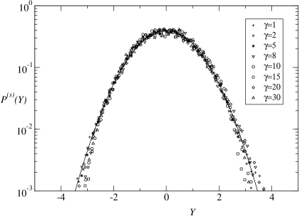
Figure 1: Steady probability distribution $P^{(s)}(Y)$ of the dimensionless variable $Y$ defined in Eq. (28). The symbols are Monte Carlo simulation results obtained with different values of $\gamma$, as indicated in the insert. The solid line is the Gaussian theoretical prediction.

In order to compare the results derived for the model in this Section with some experimental findings, it is convenient to consider also the volume fraction $\phi$ defined as $\phi\equiv l^{-1}$. As a consequence of $\sigma_{l}$ being proportional to $N^{-1/2}$, the probability density for $\phi$, $\omega_{\phi}(\phi)$ is also Gaussian, again in the limit of large $N$, with average and variance given by

$$\langle\phi\rangle^{(s)}=\langle l\rangle^{(s)-1},$$ (32)

and

$$\sigma_{\phi}=\frac{\sigma_{l}}{\langle l\rangle^{(s)2}}=\frac{\left[\left(\langle l\rangle^{(s)}-1\right)\left(2-\langle l\rangle^{(s)}\right)\right]^{1/2}}{N^{1/2}\langle l\rangle^{(s)2}}\,,$$ (33)

respectively. Thus Eq.  (26) is, for large $N$, equivalent to

$$\frac{1}{X}=\ln\frac{2\langle\phi\rangle^{(s)}-1}{1-\langle\phi\rangle^{(s)}}\,.$$ (34)

IV Comparison of the model predictions with some experimental results

Of course, given the simplicity of the model discussed here and its one-dimensional character, it can not be expected to quantitatively reproduce the experimental and simulation results. Nevertheless, it is interesting and illuminating to qualitatively analyze those results in the light of the model predictions.

The first experimental investigation of the volume fluctuations in the steady state of a tapped granular medium seems to be the one reported in ref. NKBJyN98 . More exactly, the property considered in that work is the density in a given region, located at a certain height of the system. Then, the volume is kept constant and the measured density changes are due to variations in the number of particles within the volume considered. The results indicated that the probability distribution of the density fluctuations exhibited in the majority of the cases a Gaussian shape, as found in the model, although some significant non-Gaussian deviations were also found, particularly near the bottom of the vibrated column. Moreover, the dependence on the number of particles of the relative variance was also the same as in the model, i.e $N^{-1/2}$ as shown in Eq. (20).

Variations in the inverse of the compactivity were also measured, by using the relationship between the second moment of the volume fluctuations $\sigma_{V}^{2}$ and the compactivity following from Edwards’ theory, i.e. the generalization of Eq. (22). To do so, the authors considered the specific volume $v$ defined as the inverse of the packing fraction. This corresponds to the quantity $l$ in our model. The reported results are

$$\sigma_{v}^{2}=a+b\langle v\rangle^{s},$$ (35)

$$\frac{1}{X}\propto\ln(a+b\langle v\rangle^{(s)})+\text{constant},$$ (36)

where $a$ and $b$ are two dimensionless parameters. Taking into account that the available range of experimental data is rather limited and located in the proximity of the close packing limit, it can be fairly concluded that the above expressions are in qualitative agreement with the predictions of the model, namely the expressions for $\sigma_{l}$ and $X^{-1}$, Eqs. (34) and (26) respectively. Nevertheless, to put this comparison in a fair proper context, the following two comments seem appropriated:

1. In ref. NKBJyN98 , the Edwards theory is considered in a local form, i.e. it is assumed that the state of each subregion of the system in which measurements are carried out is described by a canonical distribution with a different value of the compactivity. Although this might be a sensible idea, it is clearly an extension of the theory as originally formulated by Edwards.

2. Moreover, what is measured in the reported experiments are the fluctuations in the number of particles at constant volume. This is different from the fluctuations in the volume at constant number of particles, although both can be associated to density fluctuations. In fact, it can be shown that the quantity actually obtained from the second moment of the number of particles fluctuations by means of a relationship similar to Eq. (22) is not the compactivity, but some kind of ‘fugacity’ ByP03a . Although both quantities are simply related and perhaps their values are very close in real granular systems, they are conceptually quite different.

Another experimental study of the steady volume fluctuations in a granular medium has been carried out by Schröter et al. SGyS05 . This work might look as quite similar to the one discussed above, but they differ in important aspects, both in the methodology and in the results. In ref. SGyS05 , the fluctuations of the total volume of the system were measured, although the results are expressed in terms of the volume fraction $\phi$. A Gaussian distribution was found in all the reported cases. Also, the ratio between the standard deviation and the average turned out to be proportional to the inverse of the square root of the number of particles. Both results are the same as derived above for the model considered here. Nevertheless, the variance of the volume fraction fluctuations did not show the analogous of the simple linear behavior reported in ref. NKBJyN98 that, as it has been already mentioned, is consistent with the linear behavior predicted by Eq. (34) near the close packing limit. Instead, it presents a well defined minimum. A first, naive explanation is provided by the fact that a wider density range is analyzed in SGyS05 than in NKBJyN98 . Then, it could be expected that the linear law in the latter corresponds to an approximate description of a small window of the density interval considered in the former, namely to one with the largest volume fraction values. Even assuming this explanation, the origin of the minimum would remain as an open question.

The result obtained with the model, Eq. (34), when considered over the density range $1/2\leq\langle\phi\rangle^{(s)}\leq 1$, also shows a non-monotonic behavior, but presenting a maximum instead of a minimum exhibited by the experimental data in ref. SGyS05 . Then, it seems plausible to conclude that the existence of the minimum, if confirmed, must be due to some effects that are not captured by the simple model considered here. Given that it appears for high values of the density, it is tempting to speculate whether the increase of the volume fluctuations in that region, to the right of the minimum, is an indication of the presence of some ‘singular’ behavior associated, for instance, with the existence of a maximum random packing, a phenomenon that is not present in the model.

The Edwards compactivity $X$ was also determined by Schröter et al. by means of the granular version of the equilibrium fluctuation-dissipation theorem. To get explicit values for $X$, these authors assume that the inverse of the compactivity vanishes in the random loose packing limit. Since $X$ is a monotonic decreasing function of the volume fraction, this boundary condition implies that it is always positive. As it has already been indicated, there is nothing in the granular statistical mechanics theory requiring this to be true. If attention is restricted to the parameter region in which the model has positive compactivity, i.e. $\langle\phi\rangle^{(s)}>2/3$, the shape of the curve $X(\langle\phi\rangle^{(s)})$, Eq. (34), is similar to the one reported in Fig. 4(c) of ref. SGyS05 .

Although the recent results presented in ref. CCyN06 have not been obtained experimentally, but by means of molecular dynamics and Monte Carlo simulations, they deserve special attention because of their relevance and the interest of the analysis carried out. In particular, interest is focused on a parameter defined as the ’configurational granular temperature’, instead of the compactivity, although some close relationship between both parameters is claimed to hold. A model system of grains with normal and tangential forces is considered. The instantaneous volume fraction is measured in the steady state and analyzed as a function of its average value. To measure them, a region in the bulk of the system is considered. It is important to stress that this region is defined in such a way that both its volume and its number of particles fluctuate in time. Consistently with all the results discussed above and the model predictions, Gaussian fluctuations of the volume fraction are also found in the simulations.

The analysis of the results in CCyN06 differs, at least conceptually, of the thermodynamic theory as proposed initially by Edwards EyO89 . Instead of considering that the macroscopic parameter characterizing the state of the system is the volume, the energy is used like in normal molecular systems. More precisely, the probability $p^{(s)}_{r}$ of finding the system in the blocked metastable state $r$ of energy $E_{r}$ is assumed to be given by CyN01 ; FNyC02

$$p^{(s)}_{r}\propto e^{-E_{r}/T_{\text{conf}}},$$ (37)

where $T_{\text{conf}}$ is referred to as the configurational granular temperature of the system. The above expression is to be compared with Edwards’ proposal, see also Eq. (18),

$$p_{r}^{(s)}\propto e^{-V_{r}/X},$$ (38)

$V_{r}$ being the volume of the system in the configuration $r$. Both expressions only become equivalent if, for the relevant configurations, i.e. those with a non-vanishing probability, the energy and the volume are proportional EPAPS , with a configuration-independent constant. Consequently, the configurational temperature $T_{\text{conf}}$ and the compactivity $X$ also would be proportional in this case.

In the paper, the authors plot (fig. 4) the standard deviation $\sigma_{\phi}$ of the volume fraction fluctuations as a function of the steady average volume fraction $\langle\phi\rangle^{(s)}$. In the plotted interval, a linear behavior of $\sigma_{\phi}(\langle\phi\rangle^{(s)})$ is clearly identified. Then, by using the relationship between $\sigma_{\phi}$ and the compactivity $X$, an analytical expression of the form ByP07b

$$\frac{1}{X}=c+f(\langle\phi\rangle^{(s)})$$ (39)

is obtained. Here, the explicit form of the function $f(\langle\phi\rangle^{(s)})$ is known, while $c$ is an unknown constant. If $T_{\text{conf}}=dX$, with $d$ a constant, Eq. (39) yields

$$f(\langle\phi\rangle^{(s)})=\frac{d}{T_{\text{conf}}}-c.$$ (40)

In ref. CCyN06 , a plot of the volume fraction as a function of the configurational temperature, obtained by means of Monte Carlo simulation, is also provided (fig. 5). Consistently, this plot covers the same density range as the one giving the fluctuations. Therefore, it is posible to check whether the linearity between $f(\langle\phi\rangle^{(s)})$ and $T_{\text{conf}}^{-1}$ predicted by Eq. (40) is verified. When this is done, a systematic but quite small deviation from linearity is observed. Then, taking into account possible numerical errors as well as the fact that the measurements are carried out in such a way that both the volume considered and the number of particles inside it fluctuate, no definite conclusion can be reached on the equivalence of the canonical distribution in energy, Eq. (37), and volume, Eq. (38) ByP07b . This is an important point, both from fundamental and applied perspectives and deserves further attention.

V Linear response. Volume autocorrelation function

In this Section, the linear response of the model to a perturbation of the parameter $\gamma$, introduced below Eq. (5) will be studied. This parameter measures the ratio of the transition rates of the processes associted with hole annihilation and creation, respectively. Because of the definition in Eq. (17), a change in $\gamma$ is equivalent to modifying the compactivity $X$. In the context of real experiments, it might correspond to varying the vibration intensity, defined as the ratio between the peak acceleration of the shakes and the gravity acceleration KFLJyN95 .

The typical relaxation experiment to be considered is as follows. The system is initially prepared in a uniform density configuration corresponding to a low density state, namely with $N_{H}=N$. Then, it is allowed to evolve with a value $\gamma+\Delta\gamma$ of the rate ratio, until it reaches a steady state with a probability distribution $p^{(s)}({\bm{n}};\gamma+\Delta\gamma)$. At a given moment, taken as the time origin $t=0$, the rate ratio is instantaneously changed to the value $\gamma$. It is assumed that $|\Delta\gamma|\ll\gamma$. Then, the relaxation of the system to a new steady state $p^{(s)}({\bm{n}};\gamma)$ is followed.

The probability distribution function of the system at $t=0$ is

$$p({\bm{n}},t=0)=p^{(s)}({\bm{n}};\gamma+\Delta\gamma)\approx p^{(s)}({\bm{n}};\gamma)+\frac{\partial p^{(s)}({\bm{n}};\gamma)}{\partial\gamma}\Delta\gamma.$$ (41)

Using Eq. (18), it is obtained

$$\frac{\partial p^{(s)}({\bm{n}};\gamma)}{\partial\gamma}=\frac{\partial p^{(s)}({\bm{n}};\gamma)}{\partial X}\frac{dX}{d\gamma}=\frac{N_{H}-\langle N_{H};\gamma\rangle^{(s)}}{X^{2}}\,p^{(s)}({\bm{n}};\gamma)\frac{dX}{d\gamma}\,.$$ (42)

The average value of a function $F({\bm{n}})$ of the system configuration at time $t>0$ is, by definition,

$$\langle F,t\rangle\equiv\sum_{\bm{n}}F({\bm{n}})p({\bm{n}},t);$$ (43)

where the probability distribution $p({\bm{n}},t)$ is obtained from $p({\bm{n}},t=0)$ through

$$p({\bm{n}},t)=\sum_{{\bm{n}}^{\prime}}p({\bm{n}},t|{\bm{n}}^{\prime},0)p({\bm{n}}^{\prime},t=0).$$ (44)

Here, $p({\bm{n}},t|{\bm{n}}^{\prime},0)$ is the conditional probability that the configuration of the system is ${\bm{n}}$ at time $t$ given it was ${\bm{n}}^{\prime}$ at $t=0$. By construction, $p^{(s)}({\bm{n}};\gamma)$ is stationary for the dynamics occurring for $t>0$, i.e. with rate ratio $\gamma$,

$$\sum_{{\bm{n}}^{\prime}}p({\bm{n}},t|{\bm{n}}^{\prime},0)p^{(s)}({\bm{n}}^{\prime};\gamma)=p^{(s)}({\bm{n}};\gamma).$$ (45)

Taking this into account and using Eqs. (41) and (42), Eq. (43) becomes

$$\langle F,t\rangle=\langle F;\gamma\rangle^{(s)}+\frac{1}{X^{2}}\frac{dX}{d\gamma}\,\langle\Delta F(t)\Delta L(0);\gamma\rangle^{(s)}\Delta\gamma,$$ (46)

where $\langle\Delta F(t)\Delta L(0);\gamma\rangle^{(s)}$ is the steady time correlation function of $F({\bm{n}})$ and the volume $L$ defined as

$$\langle\Delta F(t)\Delta L(0);\gamma\rangle^{(s)}=\sum_{\bm{n}}\sum_{{\bm{n}}^{\prime}}\Delta F({\bm{n}})p({\bm{n}},t|{\bm{n}}^{\prime},0)\Delta L({\bm{n}}^{\prime})p^{(s)}({\bm{n}}^{\prime};\gamma),$$ (47)

with

$$\Delta F({\bm{n}})=F({\bm{n}})-\langle F;\gamma\rangle^{(s)},$$ (48)

$$\Delta L({\bm{n}})=L({\bm{n}})-\langle L;\gamma\rangle^{(s)}.$$ (49)

The normalized relaxation function for the property $F$, $\Phi_{F}(t)$ is

$$\Phi_{F}(t)\equiv\frac{\langle F;t\rangle-\langle F;\gamma\rangle^{(s)}}{\langle F,0\rangle-\langle F;\gamma\rangle^{s}}=\frac{\langle\Delta F(t)\Delta L(0);\gamma\rangle^{(s)}}{\langle\Delta F\Delta L;\gamma\rangle^{(s)}}\,.$$ (50)

For the special choice $F=L$,

$$\Phi_{L}(t)=\frac{\langle\Delta L(t)\Delta L(0);\gamma\rangle^{(s)}}{\sigma_{L}^{2}}.$$ (51)

This expression is an exact consequence of modelling the dynamics of the system by means of a Markov process and of the canonical form of the steady probability distribution. The Monte Carlo simulation results for the relaxation function to be presented in the following, have been obtained by using Eq. (51). Figures 2, 3, and 4 show $\Phi_{L}(t)$ for three values of the rate ratio, namely $\gamma=5$, $15$, and $50$, respectively. Other values have also been investigated, and the results are consistent with the comments carried out below. In the figures the quantity $\ln(-\ln\Phi_{L})$ has been plotted as a function of $\ln t$. It turns out that this is a convenient representation to identify the shape of the decay of $\Phi_{L}(t)$. Note that in this representation, a straight line corresponds to a stretched exponential or Kohlrausch-Willians-Watts (KWW) function,

$$\Phi_{KWW}(t)=\exp\left[-\left(\frac{t}{\tau}\right)^{\beta}\right],$$ (52)

where $\tau$ and $\beta$ are the two parameters identifying the function.

In the three figures, two different regions are easily identified. For ‘short’ times, there is a linear region with slope $\beta\approx 1$. i.e. an exponential decay. Afterwards, there is a region of ‘intermediate’ times in which another linear behavior shows up, but now with $\beta<1$. The initial region extends over a time interval, $\ln t\lesssim 2$, that is roughly independent of $\gamma$. In this time interval, the response function $\Phi_{L}$ decays a small amount. Moreover, this initial decay becomes smaller and smaller as the value of $\gamma$ increases. On the other hand, in the second time window in which the response function shows a KWW behavior, most of the relaxation occurs. For $\gamma=5$, Fig. (2), the fit to a KWW function with $\beta\simeq 0.659$ is quite good for the time interval $3\lesssim\ln t\lesssim 6$, that corresponds to $-2\lesssim\ln(-\ln\Phi_{L})\lesssim 0.75$, i.e. $0.87\gtrsim\Phi_{L}\gtrsim 0.12$. For $\gamma=15$, Fig. 3, the value of $\beta$ in the intermediate time window is $\beta\simeq 0.567$, and the interval of the relaxation function described by it is $0.92\gtrsim\Phi_{L}\gtrsim 0.12$. Finally, for $\gamma=50$, Fig. 4, it is $\beta\simeq 0.534$ for $0.95\gtrsim\Phi_{L}\gtrsim 0.12$.

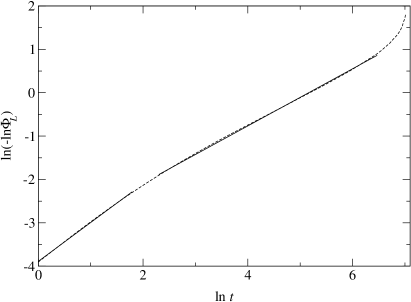
Figure 2: Double logarithm plot of the normalized response function for the volume as a function of the logarithm of the time for $\gamma=5$. The latter is measured in dimensionless units proportional to the number of Taps. The dashed line is the Monte Carlo simulation result, while the two solid lines are linear fits as discussed in the text.

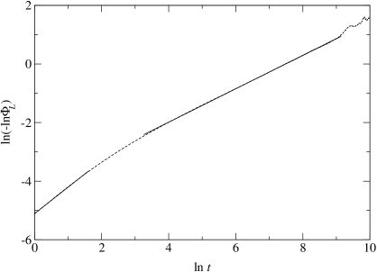
Figure 3: The same as Fig. 2, but for $\gamma=15$.

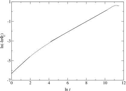
Figure 4: The same as Fig. 2, but for $\gamma=50$.

The kind of behavior of the response function has been often found in the context of structural glasses, both in experiments and in simple models, for the linear relaxation of the energy following a temperature perturbation Sch86 ; Fr88 ; ByP96 . Then, this is another indication of a possible conceptual connection between structural glasses and dense granular systems. Moreover, the simulation results for the model clearly indicate that the value of the exponent $\beta$ characterizing most of the relaxation tends to $1/2$ as the value of $\gamma$ increases. In simple models of structural glasses, this value is associated to diffusive processes ByP96 ; BPyR94 .

Although an explicit analytical solution of the model has not been derived yet, it is possible to understand the diffusive origin of the exponent $\beta=1/2$ as well as to get some information about the characteristic relaxation time $\tau$. For $\gamma\gg 1$ ($X\ll 1$), a typical metastable configuration of the system consists of isolated holes separated a distance of the order of $\gamma$ (see, for instance, Eq. (15)). In this situation, the only relevant process to decrease the volume is diffusion: holes move through the system until two of them get together and one is destroyed. In this picture, the characteristic relaxation time will have the diffusion form $\tau\propto\gamma^{2}=e^{2/X}$, i.e. an Arrhenius type law with the molecular temperature replaced by $X$.

In Fig. 5, the Monte Carlo simulation results for $\tau$, obtained by fitting the relevant intermediate time window to a KWW function as discussed above, are plotted as a function of $\gamma$. Note the logarithmic scale, so that the observed straight line represents a power law behavior. The best fit, given by the solid line, yields $\tau\approx 6.87\gamma^{2.04}$ in good agreement with the result following from the diffusive picture.

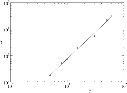
Figure 5: Plot of the relaxation time $\tau$ appearing in the KWW expression, Eq. (52), as a function of the rate ratio $\gamma$. Time is measured in units proportional to the number of taps. The symbols are from the Monte Carlo simulation data and the solid line a linear fit of them.

VI Conclusion

A simple model for compaction in granular media has been used to investigate some static and dynamic properties of the steady sate reached by the system in the long time limit. The simplicity of the model allows to obtain analytical expressions for some of its properties. On the other hand, it reproduces qualitatively well many of the properties found in real granular systems. In the context of static properties, this includes the Gaussian shape of the volume fluctuations, the dependence of its variance on the average volume and the number of particles, and the possibility of identifying the compactivity as defined by Edwards.

Moreover, the scenario obtained from the analysis of the model, provides an useful tool to interpret the experimental results and molecular dynamic simulations of more realistic models. This is exemplified in the critical revision carried out in Sec. IV, where the need of a clear differentiation between density fluctuations at constant volume and at constant number of particles shows up. Also, attention must be paid to distinguish between local and global applications of the thermodynamic theory.

Another issue that is worth commenting is the possible existence of negative values of the compactivity and/or the effective temperature. If the mechanical statistical description is assumed as the starting point of a thermodynamic description, there is no solid reason to deny by principle this possibility. Even more, one is tempted to conclude that it is highly probable, at least at a theoretical level. Negatives values of the compactivity will show up unavoidably if the number of metastable configurations is not a monotonic increasing function of the volume. The possible volume occupied by the tapped granular medium is limited by the loose and random jamming packings. In both limits, the number of possible metastable configurations can be expected to be quite reduced. The requirement of maximum or minimum space between particles impose a rather severe restriction on the allowed arrangement of the particles. Therefore, it seems sensible to expect that the number of configurations for intermediate values of the volume be larger than at the extremes, presenting a maximum at some values. The same qualitative reasoning applies to the effective or configurational temperature changing the volume by the energy.

The question then is why negative compactivities (effective temperatures) have been not identified in the experiments yet. There are two main reasons for it. The first one is that only differences of compactivities have been measured up to now, and it has often been arbitrarily assumed that the compactivity diverges in the random loose packing limit. The second reason is that negative values of the compactivity, if they exist, would correspond to the lowest density theoretically accesible region, and it can be very hard to reach in practice. In any case, this is a point that definitely deserves much more study.

In the last part of the paper, the linear relaxation of the model has been considered. A slow relaxation, accurately represented by a KWW function with exponent $\beta$ tending to $1/2$ as the parameter corresponding to the vibration intensity is decreased, has been found. Moreover, the expression of the characteristic relaxation time $\tau$ has Arrhenius form (with the consistent substitution of the compactivity by the temperature).

The behavior of the linear response function for the model is fully similar to what is observed in the relaxation of many structural glasses and also in models of glassy relaxation. It must be noted that the model discussed here was built to mimic the compaction experiment and that, consistently, the relaxation of the density starting from a loose configuration exhibits the characteristic inverse logarithmic law ByP03a found in experiments KFLJyN95 ; NKBJyN98 . It seems interesting to experimentally investigate whether linear response in tapped granular systems is also slow and described by a KWW function. If that were the case, it would be another indication of similarity between two apparently different kind of systems, granular media and structural glasses, reinforcing the link already found in other phenomena GyS06 , including the existence of hysteresis cycles NKBJyN98 ; PByS00 and memory effects JTMyJ00 ; ByP02 .

- (1) G.C. Parker and A. Mehta, Phys. Rev. A 45, 3435 (1993).
- (2) J.B. Knight, C.G. Fandrich, C.N. Lau, H.M. Jaeger, and S.R. Nagel, Phys. Rev. E 51, 3957 (1995).
- (3) S. F. Edwards and R. B. S. Oakeshott, Physica A 157, 1080 (1989); S. F. Edwards and A. Metha, Journal de Physique 50, 2489 (1989); S. F. Edwards and C. C. Mounfield, Physica A 210, 279 (1994).
- (4) E.R. Nowak, J.B. Knight, E. Ben-Naim, H.M Jaeger, and S.R. Nagel, Phys. Rev. E 57, 1971 (1998).
- (5) P. Philippe and D. Bideau, Europhys. Lett. 60, 677 (2002).
- (6) M. Schröter, D.J. Goldman, and H.L. Swinney, Phys. Rev. E 71, 030301(R) (2005).
- (7) H. A. Makse and J. Kurchan, Nature 415, 614 (2002).
- (8) M.P. Ciamarra, A. Coniglio, and M. Nicodemi, Phys. Rev. Lett. 97, 158001 (2006).
- (9) A. Barrat, J. Kurchan, V. Loreto, and M. Sellitto, Phys. Rev. Lett. 85, 5034 (2000); A. Barrat, J. Kurchan, V. Loreto, and M. Sellitto, Phys. Rev. E 63, 051301 (2001); V. Colizza, A. Barrat, and V. Loreto, Phys. Rev. E 65, 050301 (2002).
- (10) A. Fierro, M. Nicodemi and A. Coniglio, Europhys. Lett. 59, 642 (2002).
- (11) D. S. Dean and A. Lefevre, Phys. Rev. Lett. 90, 198301 (2003).
- (12) J. J. Brey, A. Prados, and B. Sánchez-Rey, Phys. Rev. E 60, 5685 (1999); Physica A 275, 310 (2000).
- (13) A. Léfevre and D. S. Dean, J. Phys. A 34, L213 (2001).
- (14) J. Berg, S. Franz, and M. Sellito, Eur. Phys. J. B 26, 349 (2002).
- (15) G. De Smedt, C. Godreche, and J. M. Luck, Eur. Phys. J. B 27, 363 (2002).
- (16) A. Prados and J. J. Brey, Phys. Rev. E 66, 041308 (2002).
- (17) J.J. Brey and A. Prados, Phys. Rev. E 68, 051302 (2003).
- (18) A. Coniglio and M. Nicodemi, Physica A 296, 451 (2001).
- (19) E.R. Nowak, J.B. Knight, M. Povinelli, H.M. Jaeger, and S.R. Nagel, Powder Technol. 94, 79 (1997).
- (20) N.G. van Kampen Stochastic Processes in Physics and Chemistry (North-Holland, Amsterdam, 1992).
- (21) R. Monasson and O. Pouliquen, Physica A 236, 395 (1997).
- (22) EPAPS Document No. E-PRLTAO-97-045642. For information on EPAPS, see http://www.aip.org/pubservs/epaps.html.
- (23) J.J. Brey and A. Prados, unpublished.
- (24) See, for instance, G.W. Schrerer, Relaxation in Glass and Composites (Wiley, New York, 1986).
- (25) G.H. Fredrickson, Annu. Rev. Phys. Chem. 39, 149 (1988).
- (26) J.J. Brey and A. Prados, Phys. Rev. E 53, 458 (1996).
- (27) J.J. Brey, A. Prados, and M.J. Ruiz-Montero, J. Non-Cryst. Solids 172-174, 371 (1994).
- (28) D.I. Goldman and H.L. Swinney, Phys. Rev. Lett. 96, 145702 (2006).
- (29) A. Prados, J.J. Brey, and B. Sánchez-Rey, Physica A 284, 277 (2000).
- (30) C. Josserand, A. Tkachenko, D.M. Mueth, and H.M. Jaeger, Phys. Rev. Lett. 85, 3632 (2000).
- (31) J.J. Brey and A. Prados, Europhys. Lett. 57, 171 (2002).