Magnetic circular dichroism in EELS: Towards 10 nm resolution

Abstract

We describe a new experimental setup for the detection of magnetic circular dichroism with fast electrons (emcd). As compared to earlier findings the signal is an order of magnitude higher, while the probed area could be significantly reduced, allowing a spatial resolution of the order of 30 nm. A simplified analysis of the experimental results is based on the decomposition of the Mixed Dynamic Form Factor $S(\vec{q},\,\vec{q}^{\prime},E)$ into a real part related to the scalar product and an imaginary part related to the vector product of the scattering vectors ${\vec{q}}$ and ${\vec{q}^{\prime}}$. Following the recent detection of chiral electronic transitions in the electron microscope the present experiment is a crucial demonstration of the potential of emcd for nanoscale investigations.

1 Introduction

The observation of circular dichroism with electron probes has been considered impossible except with spin polarized electron probes. In 2003 it was suggested that this was not the case [1]. The magnetic transitions that give rise to X-ray magnetic circular dichroism (xmcd) contribute to the imaginary part of the Mixed Dynamic Form Factor (mdff) [2] for inelastic electron scattering. Since this quantity can be measured in the transmission electron microscope (tem) under particular scattering conditions, we predicted that detection of xmcd should be feasible in the tem. We called the predicted effect Energy-Loss Magnetic Chiral Dichroism (emcd).

In the first conclusive experimental demonstration of emcd on Fe [3] it was discovered that the effect is smaller than xmcd. In that experiment the dichroic signal was close to the noise threshold in the then chosen geometry and the area of investigation was approximately 100 nm in radius.

Here we present a new experimental setup that enhances the count rate by an order of magnitude and reduces the probed area by another factor of five, thus opening the way to applications of emcd on the nanometric scale.

The mdff $S({\vec{q}},{\vec{q}}^{\prime},E)$ is the essential quantity describing emcd. It has been used in the description of interference of inelastically scattered electrons (e. g. [2, 4, 5]).

2 The Mixed Dynamic Form Factor (MDFF)

The semi-relativistic double differential scattering cross section for inelastic electron scattering (DDSCS) in the plane wave Born approximation is [6]

$$\frac{\partial^{2}\sigma}{\partial E\partial\Omega}=\frac{4\gamma^{2}}{a_{0}^{2}\,q^{4}}\frac{k_{f}}{k_{i}}S({\vec{q}},E)$$ (1)

where $a_{0}$ is the Bohr radius, $k_{i}$ $(k_{f})$ is the wave number of the incident (outgoing) probe electron, ${\vec{q}}={\vec{k}}_{i}-{\vec{k}}_{f}$ is the wave vector transfer in the interaction and $E$ the energy loss. $S({\vec{q}},E)$ is the dynamic form factor (dff).

Interference between inelastically scattered electrons in the diffraction pattern will occur when the probe electron consists of two or more mutually coherent plane waves [4, 7]. Experimentally, this can be realized by a biprism [8] or by any other beam splitter. It was shown experimentally that the crystal itself can be used as a beam splitter for inelastic electron scattering [9]. In the crystal the probe electron is a superposition of Bloch waves which, in turn, are coherent superpositions of plane waves defined by the allowed Bragg reflections.

For the sake of clarity, we consider the simplest case here, namely the superposition of two plane waves with complex amplitudes $A_{1,\,2}$, respectively. Technically, this situation is approximated in electron diffraction by the two-beam case, the most important plane waves being the incident one and a single Bragg scattered wave.

The DDSCS is then [2]

$$\frac{\partial^{2}\sigma}{\partial E\partial\Omega}=\frac{4\gamma^{2}}{a_{0}^{2}}\frac{k_{f}}{k_{i}}\big{(}|A_{1}|^{2}\frac{S({\vec{q}},E)}{q^{4}}+|A_{2}|^{2}\frac{S({\vec{q}}\,^{\prime},E)}{q^{\prime 4}}+2\Re[A_{1}A_{2}^{\ast}\frac{S({\vec{q}},{\vec{q}}\,^{\prime},E)}{q^{2}q^{\prime 2}}]\big{)}.$$ (2)

Here, ${\vec{q}}={\vec{k}}_{i}-{\vec{k}}_{f}$, ${\vec{q}}\,^{\prime}={{\vec{k}}^{\prime}}_{i}-{\vec{k}}_{f}$ are the wave vector transfers from the two incident plane waves ${\vec{k}}_{i},\,{{\vec{k}}^{\prime}}_{i}$ to ${\vec{k}}_{f}$. Since i) the $2p$ $\to$ $3d$ transitions are the dominant ones due to the shape of the density of states and ii) due to the localized character of $<i|$, the matrix elements $\langle i|e^{i{\vec{q}}{\vec{R}}}|f\rangle$ are mostly determined by an area within small $R$ values (compared to lattice parameters), we can use the dipole approximation for the mdff [4]

$$S({\vec{q}},{\vec{q}}\,^{\prime},E)_{\text{dip}}=\sum_{if}\langle i|{{\vec{q}}{\vec{R}}}|f\rangle\langle f|{{\vec{q}}\,^{\prime}{\vec{R}}}|i\rangle\delta(E+E_{i}-E_{f}).$$ (3)

${\vec{R}}$ is the 3-vector operator $(r_{1},r_{2},r_{3})$ of the one-electron scatterer with initial and final wave functions $|i\rangle$, $|f\rangle$.

Eq. 2 consists of two direct terms, each resembling the angular scattering distributions centered at the incident and the Bragg scattered plane wave directions, and an interference term. Eq. 2 is formally equivalent to the expression for intensity in the double slit experiment. It should be noted that the diagonal element of the mdff is the dff, $S({\vec{q}},{\vec{q}},E)=S({\vec{q}},E)$.

The mdff describes the mutual coherence of transitions with energy transfer $E$ and momentum transfer $\hbar{\vec{q}},\hbar{\vec{q}}^{\prime}$ [4] (Two different momentum transfers can occur in one transition with finite probability when the incident or the outgoing electron is not a single plane wave. In the present case $A_{1}|{\vec{k}_{i}}\rangle+A_{2}|{\vec{k}^{\prime}}_{i}\rangle$ is such a basis function, and the measurement collapses the probe electron into $|{\vec{k}}_{f}\rangle$ ).

With the matrix elements

$$r_{jk}=\sum_{if}\langle i|r_{j}|f\rangle\langle f|r_{k}|i\rangle\delta(E+E_{i}-E_{f}).$$ (4)

of the transition matrix ${\hat{R}}=\{r_{jk}\}$ the mdff, eq. 3 can be written as

$$S({\vec{q}},{\vec{q}}\,^{\prime},E)_{dip}={\vec{q}}{\hat{R}}{\vec{q}}\,^{\prime}\,.$$ (5)

For isotropic systems the transition matrix degenerates to a quantity proportional to the unity matrix [2]. This case was discussed in the context of ionisation fine structure and dynamical diffraction  [10, 7].

Anisotropy can be induced by a lattice of lower than cubic symmetry, or by magnetic fields. These can be internal or external, then speaking of natural or magnetic dichroism [11]. It is well known that with photon scattering linear as well as circular dichroism can be measured. This technique is largely applied with external magnetic fields. Linear magnetic dichroism shows up as an uniaxial anisotropy and can be measured with angle resolved inelastic electron scattering, tuning $\vec{q}$ parallel or perpendicular to the anisotropy axis. This is equivalent [12] to the tuning of linear polarization of the photon in xanes experiments.

It has been thought that circular magnetic dichroism cannot be detected with electrons except with spin polarized ones. But let us recall that in xanes the photon does not couple directly to the spin of electrons but to the angular momentum of the excited atom, and the effect becomes visible by the spin-orbit coupling [11]. So there is no reason that spin polarized electrons are needed for detection of circular dichroism in electron energy loss spectrometry (eels). Rather, in the inelastic electron interaction that is equivalent to an xmcd experiment, the virtual photon that is exchanged must be circularly polarized.

The mdff, eq. 5 can be written in a different form when we specify the magnetic field direction as the positive $r_{3}$ axis  and write ${\vec{q}}=({\vec{q}}_{\perp},q_{3})$. A little algebra shows that

$$S({\vec{q}},{\vec{q}}\,^{\prime},E)_{dip}=\frac{1}{2}({\rm r}_{++}+{\rm r}_{--})\,{\vec{q}}_{\perp}\cdot{\vec{q}}_{\perp}\,^{\prime}+{\rm r}_{00}\,q_{3}q^{\prime}_{3}+\frac{i}{2}({\rm r}_{++}-{\rm r}_{--})\,({\vec{q}}_{\perp}{\times}\,{\vec{q}}_{\perp}\,^{\prime})\cdot{\vec{e}_{3}}$$ (6)

where ${\vec{e}_{3}}$ is the unit vector in direction of the $r_{3}$ axis, and we have used the transition matrix elements in terms of the spherical components $R_{+,\,-,\,0}$ of the 3-space operator

$${\rm r}_{++}=\sum_{if}\langle i|R_{+}|f\rangle\langle f|R_{+}|i\rangle\delta(E+E_{i}-E_{f}).$$ (7)

and similar for all other combinations. They relate to the Cartesian components by the transformation rules for vector spherical harmonics [13]. All matrix elements and vector components are real in eq. 6. In this form we have separated the mdff into a real component proportional to the scalar product of the wave vector transfers ${\vec{q}}_{\perp},\,{\vec{q}}\,^{\prime}_{\perp}$ and an imaginary part proportional to their vector product. This structure is equivalent to that of the polarization tensor used in xmcd, which decomposes into a scalar part (uneffective in dichroic experiments), a second-rank irreducible part detectable by linear dichroism and a pseudovector part sensitive to magnetic moments [11, 14] and reference therein.

This form of the MDFF allows a description of the scattering geometry for emcd detection in the tem. In passing we note that the imaginary part vanishes if the magnetic transitions ($\Delta m=\pm 1$) are degenerate. Only when the presence of a magnetic field in $r_{3}$ direction lifts the $m$-degeneracy will we see an effect. For a transition with fixed energy loss $E$ the operators $R_{+}$ and $R_{-}$ will then contribute with different oscillator strengths, and the mdff eq. 6 will acquire an imaginary part. Its sign depends on which transitions are allowed by the selection rules.

The imaginary part can be interpreted as the difference in probability to change the magnetic quantum number by $\pm 1$. It thus describes the difference in response of the system to left- respectively right-handed circularly polarized electromagnetic fields .

The scattering vector ${\vec{q}}_{\perp}$ in the diffraction plane is perpendicular to the magnetic field vector. We assumed already that the magnetic moments of the scatterer are aligned parallel to the optical axis $r_{3}$ in the strong magnetic field ($\approx$ 2 T) of the objective lens of the microscope. We can now evaluate the DDSCS for specimens showing magnetic circular dichroism.

If in eq. 2 we write the phase shift $\phi$ explicitly as $A_{1}A_{2}^{\ast}=|A_{1}||A_{2}|\cdot e^{-i\phi}$, inspection of eq. 6 then reveals that a phase shift $\phi\neq n\pi$ between the two incident plane waves is needed in order to activate the imaginary part of the mdff. A phase shift of $\pm\pi/2$ is recommended since in this case the real part of the mdff disappears in eq. 2, and only the imaginary part survives. In a two-beam case with such a phase shift the pseudovector part contributes with its full magnitude and gives rise to an asymmetry in the scattering cross section of a magnetic transition such as the L edges of the ferromagnetic d-metals.

3 Experiments and simulations

We performed our experiment on a Co single crystal electropolished sample with a FEI Tecnai F20-FEGTEM S-Twin operating at 200 keV and equipped with a Gatan imaging filter (GIF). The dichroic signal is obtained by first tilting out of the [0001] zone axis to a two-beam case where only the $0000$ and $10\bar{1}0$ reflections are strongly excited. Following the procedure illustrated in [3], a selected area aperture (SAA) is used to delimit a region of about 100 nm radius and 18 $\pm$ 3 nm thickness. The corresponding diffraction pattern is then projected onto the 2 mm spectrometer entrance aperture (SEA). Drawing a circle with a diameter of G with the 0- and G-reflections on the left and right side respectively, the strongest dichroic signal can be expected at the top and bottom points A and B of this Thales circle (fig. 1) where the scalar product ${\vec{q}}\cdot{\vec{q}}\,^{\prime}$ is zero and the pseudovector ${\vec{q}}\times{\vec{q}}\,^{\prime}$ maximises the imaginary part of the mdff. The camera lenght and projection coils are then adjusted so that the SEA will be centered at these two points (first A, then B) in the Thales circle and determine a collection angle of 2-4 mrad. Two spectra are then acquired sequentially (fig. 2). With an acquisition time of 60 sec per spectrum and an energy dispersion of 0.5 eV/channel the intensity at the $L_{3}$ peak was about 2,500 counts (after background removal).

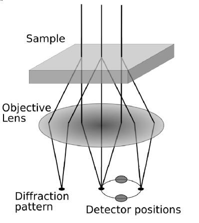
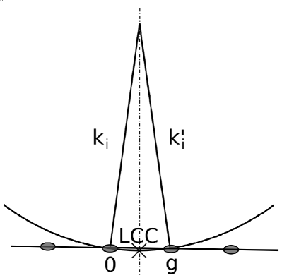
Figure 1: Left: the electron beam creates a diffraction pattern in the focal plane of the objective lens. Placing the SEA in the diffraction plane will select one direction for the outgoing electron beam. The red circles indicate positions A and B of our experimental setup. Right: in reciprocal space the Ewald sphere is defined by the incident wave vector $\bf k_{i}$. If a reciprocal lattice vector (g) lies on the surface of the sphere, the Bragg spot will be strongly excited (as is the case for $\bf k^{\prime}_{i}$ in the figure). The projection of the sphere on the diffraction plane is called Laue Circle Centre (LCC, equal to g/2 in the figure).

Figure 2: EELS spectra of the Co $L_{2,3}$ edge showing EMCD using the detector shift method.

In order to improve the signal-to-noise ratio a new experimental setup was devised. As detailed above, the sample is tilted out of the [0001] zone axis to a two-beam case where only the $0000$ and $10\bar{1}0$ reflections are observed in the the energy filtered diffraction pattern, which is then projected onto the spectrometer entrance aperture (SEA). Using a rotational sample holder, the reciprocal lattice vector $\vec{G}$ is then aligned parallel to the energy dispersive axis of the CCD camera, so that a q-E diagram can be recorded as depicted in fig. 3. The quadrupoles of the energy filter collapse (integrating the signal in the $q_{x}$ dimension) the circular area to a line in $q_{y}$ when the system is switched to spectroscopy mode. This first modification allows us to record not only both spectra A and B with a single acquisition, but the entire range of spectra with different $q_{y}$ values comprised within the 2 mm SEA. It should be noted however that the integration area in the $q_{x}$ dimension is different for every value of $|q_{y}|$.

A second modification consists in a different method [15] to obtain a spot like inelastic diffraction pattern: the beam (with a convergence semi-angle of $\alpha=2$ mrad) is focussed onto a 18 $\pm$ 3 nm thick area of the Co specimen which is then shifted upwards from the eucentric position by $z=9.25\,\mu$m. The diameter of the illuminated area is $d=2\alpha z=37$ nm, accurate to 5%, in the present experiment (fig. 4).

Preliminary experiments show that with smaller $z$-shifts the illuminated area can be reduced to less than 10 nm radius, at the moment with untenable distortions of the diffraction pattern. With a C${}_{\text{s}}$ corrector or a monochromator a spatial resolution of 10 nm or less should be attainable.

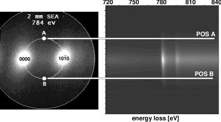
Figure 3: Left: Energy filtered diffraction pattern at 784 eV energy loss using a slit width of 20 eV. The sample was oriented in the two-beam case, capturing both reflections within the 2 mm SEA. Right: q-E diagram of the Co L_2,3 edge in chiral conditions (for details see text).

Figure 4: Geometry of the experiment: When the specimen is shifted upward from the eucentric position (Image Plane) by $z$ the illuminated area is a disk with radius $\alpha z$. Bragg scattering will cause a diffraction pattern to appear in the Image Plane.

Similarly to xmcd we define $\Delta\sigma$ as the difference between spectra with opposite helicity and $\bar{\sigma}$ as their average. The dichroic signal is then the relative difference $\Delta\sigma/\bar{\sigma}$ in the scattering cross section when the sign of the pseudovector part changes . This is obtained by tracing the spectral intensity at points A and B in fig. 3, and taking their difference, as shown in fig. 5. With an acquisition time of 15 sec and an energy dispersion of 0.3 eV/channel the intensity at the $L_{3}$ peak was about 13,500 counts (after background removal).

Figure 5: EELS spectra extracted from the q-E diagram (fig. 3) by line traces parallel to the energy axis and passing by the positions A and B. The difference is the dichroic signal stemming from $\Im(S(q,q^{\prime},E))$.

The modified scattering geometry provides a count rate per eV which is an order of magnitude higher than the one achieved in the previous configuration [3], thus improving significantly the signal to noise ratio. This is essentially caused by the fact that when no SAA is used and the beam is focussed only on the area of interest, all the electrons emitted from the gun contribute to the detected signal. In the formerly used geometry a nearly parallel incident bundle illuminated a large area of the sample of which only a small fraction could be used. This effectively reduced the intensity by which the area of interest is illuminated, i.e. a large part of the incident electrons did not contribute to the signal. The increase in the count rate per eV allows us to reduce the acquisition time, thus limiting the effects of beam instability, specimen and energy drift. The shorter acquisition time, combined with the finer energy dispersion, improves the energy resolution with which the $L_{2,3}$ edges are recorded. In the older setup the $L_{3}$ has a FWHM of 7 eV (fig. 2), compared to the 3.6 eV achieved with the new method (fig. 5).

Ab initio DFT simulations of the dichroic signal were performed using an extension [16] of the WIEN2k package [17] developped for this purpose. In the simulation the effects of thickness, tilt of the incident beam, position of the detector were included as well as the integration over $q_{x}$ in the range dictated by the use of a circular SEA. Up to 8 beams were used for the calculations of the MDFFs. A comparison with the experiment is given in fig. 6 for the $L_{3}$ edge of Cobalt. The agreement is very good between -0.8 and 0.8 G with some discrepancy appearing at larger scattering angles. This can be due to the faint Bragg spots outside the systematic row (which are neglected in the simulations) and to the fact that the SEA is not exactly in the spectral plane of the energy filter. The error bars correspond to the ($2\sigma$) Poissonian noise calculated for the theoretical signal using the number of electrons contributing to the signal as determined from the experimental data.

Figure 6: Dichroic signal at the Cobalt $L_{3}$ edge as function of the scattering angle $q$ (in unit of G) in the direction perpendicular to the Bragg scattering vector G. Positions A and B (see fig. 3) correspond to points q/G = 0.5 and -0,5 respectively. Comparison between experimental data (triangles) and ab initio simulation. The error bars correspond to simulated Poissonian noise ($2\sigma$).

4 Conclusions

The strong chiral effect observed in the Co L_2,3 edge shows that emcd can be measured with reasonable collection time in the TEM. The convergence angle of 2 mrad is obviously not detrimental for the necessary constant phase shift between the unscattered and the Bragg scattered electron waves. The $z$-shift of the specimen allows to control the illuminated area, and with optimized conditions a lower limit of $\leq$ 10 nm appears realistic. This would define the lateral resolution in scanning mode. In order to achieve this goal some technical problems such as the stability of the beam in the magnetic field, constant $z$-shift or decoupling of the scan coordinate from the positioning of the diffraction pattern must be solved. The simple concept described above should be an incentive for novel dichroic experiments in the TEM. It also shows that emcd can be complementary and competitive with traditional or new [18] XMCD techniques.

Acknowledgements:

This work was sponsored by the European Union under contract nr. 508971 (FP6-2003-NEST-A) "Chiraltem". We acknowledge Jo Verbeeck for stimulating discussions.

References

- [1] C. Hébert and P. Schattschneider, Ultramicroscopy 96, 463 (2003).
- [2] H. Kohl and H. Rose, Advances in electronics and electron optics 65, 173 (1985).
- [3] P. Schattschneider, S. Rubino, C. Hébert, J. Rusz, J. Kuneš, P. Novák, E. Carlino, M. Fabrizioli, G. Panaccione and G. Rossi, Nature 441, 486 (2006).
- [4] P. Schattschneider, M. Nelhiebel, H. Souchay and B. Jouffrey, Micron 31, 333 (2000).
- [5] P. Schattschneider and W. S. M. Werner, J. Electron Spectrosc. Relat. Phenom. 143, 81 (2005).
- [6] P. Schattschneider, C. Hébert, H. Franco and B. Jouffrey, Phys. Rev. B 72, 045142 (2005).
- [7] P. Schattschneider, M. Nelhiebel and B. Jouffrey, Phys. Rev. B 59, 10959 (1999).
- [8] H. Lichte and B. Freitag, Ultramicroscopy 81, 177 (2000).
- [9] M. Nelhiebel, P. Schattschneider and B. Jouffrey, Phys. Rev. Lett. 85(9), 1847 (2000).
- [10] M. Nelhiebel, N. Luchier, P. Schorsch, P. Schattschneider and B. Jouffrey, Philosophical Magazine B 79, 941 (1999).
- [11] S. W. Lovesey and S. P. Collins, X-Ray Scattering and Absorption by Magnetic Materials, Clarendon Press, Oxford, UK, 1996.
- [12] A. P. Hitchcock, Jpn. J. Appl. Phys. 32(2), 176 (1993).
- [13] J. P. Hannon, G. T. Trammel, M. Blume and D. Gibbs, Phys. Rev. Lett. 61, 1245 (1988).
- [14] M. Altarelli, Resonant X-ray scattering: a theoretical introduction in: E. Beaurepaire, H. Boulu, F. Scheurer and J. P. Klapper (Eds.), Magnetism: a synchrotron radiation approach, Springer, Berlin, Germany, 2006, pp. 201-242.
- [15] P. A. Midgley, Ultramicroscopy 79, 91 (1999).
- [16] J. Rusz, S. Rubino and P. Schattschneider, submitted.
- [17] P. Blaha, K. Schwarz, G. K. H. Madsen, D. Kvasnicka and J. Luitz, 2001 WIEN2k, Vienna University of Technology (ISBN 3-9501031-1-2).
- [18] S. Eisebitt, J. Lüning, W. F. Schlotter, M . Lörgen, O. Hellwig, W. Eberhardt, and J. Stöhr, Nature 432, 885 (2004).