Valence bond solids for SU() spin chains:
exact models, spinon confinement, and the Haldane gap
Abstract
To begin with, we introduce several exact models for SU(3) spin chains: (1) a translationally invariant parent Hamiltonian involving four-site interactions for the trimer chain, with a three-fold degenerate ground state. We provide numerical evidence that the elementary excitations of this model transform under representation of SU(3) if the original spins of the model transform under rep. . (2) a family of parent Hamiltonians for valence bond solids of SU(3) chains with spin reps. , , and on each lattice site. We argue that of these three models, only the latter two exhibit spinon confinement and hence a Haldane gap in the excitation spectrum. We generalize some of our models to SU(). Finally, we use the emerging rules for the construction of VBS states to argue that models of antiferromagnetic chains of SU() spins in general possess a Haldane gap if the spins transform under a representation corresponding to a Young tableau consisting of a number of boxes which is divisible by . If and have no common divisor, the spin chain will support deconfined spinons and not exhibit a Haldane gap. If and have a common divisor different from , it will depend on the specifics of the model including the range of the interaction.
pacs:
75.10.Jm, 75.10.Pq, 75.10.Dg, 32.80.PjI Introduction
Quantum spin chains have been a most rewarding subject of study almost since the early days of quantum mechanics, beginning with the invention of the Bethe ansatz in 1931 bethe31zp205 as a method to solve the Heisenberg chain with nearest-neighbor interactions. The method led to the discovery of the Yang–Baxter equation in 1967 yang67prl1312 ; baxter90 , and provides the foundation for the field of integrable models KorepinBogoliubovIzergin93 . Faddeev and Takhtajan faddeev-81pla375 discovered in 1981 that the elementary excitations (now called spinons) of the spin- Heisenberg chain carry spin while the Hilbert space is spanned by spin flips, which carry spin 1. The fractional quantization of spin in spin chains is conceptually similar to the fractional quantization of charge in quantized Hall liquids laughlin83prl1395 ; stone92 . In 1982, Haldane haldane83pla464 ; haldane83prl1153 identified the O(3) nonlinear sigma model as the effective low-energy field theory of SU(2) spin chains, and argued that chains with integer spin possess a gap in the excitation spectrum, while a topological term renders half-integer spin chains gapless affleck90proc ; Fradkin91 .
The general methods—the Bethe ansatz method and the use of effective field theories including bosonization GogolinNersesyanTsvelik98 ; Giamarchi04 —are complemented by a number of exactly solvable models, most prominently among them the Majumdar–Ghosh (MG) Hamiltonian for the dimer chain majumdar-69jmp1399 , the AKLT model as a paradigm of the gapped chain affleck-87prl799 ; affleck-88cmp477 , and the Haldane–Shastry model (HSM) haldane88prl635 ; shastry88prl639 ; haldane91prl1529 ; haldane-92prl2021 . The HSM is by far the most sophisticated among these three, as it is not only solvable for the ground state, but fully integrable due to its Yangian symmetry haldane-92prl2021 . The wave functions for the ground state and single-spinon excitations are of a simple Jastrow form, elevating the conceptual similarity to quantized Hall states to a formal equivalence. Another unique feature of the HSM is that the spinons are free in the sense that they only interact through their half-Fermi statistics haldane91prl937 ; ha-93prb12459 ; essler95prb13357 ; greiter-05prb224424 ; greiter06prl , which renders the model an ideal starting point for any perturbative description of spin systems in terms of interacting spinons greiter-06prl . The HSM has been generalized from SU(2) to SU() kawakami92prb1005 ; kawakami92prbr3191 ; ha-92prb9359 ; bouwknegt-96npb345 ; schuricht-05epl987 ; schuricht-06prb235105 .
For the MG and the AKLT model, only the ground states are known exactly. Nonetheless, these models have amply contributed to our understanding of many aspects of spin chains, each of them through the specific concepts captured in its ground state jullien-83baps344 ; affleck89jpcm3047 ; okamoto-92pla433 ; eggert96prb9612 ; white-96prb9862 ; sen-07prb104411 ; knabe88jsp627 ; fannes-89epl633 ; freitag-91zpb381 ; kluemper-91jpal955 ; kennedy-92prb304 ; kluemper-92zpb281 ; kluemper-93epl293 ; batchelor-94ijmpb3645 ; schollwock-96prb3304 ; kolezhuk-96prl5142 ; kolezhuk-02prb100401 ; normand-02prb104411 ; lauchli-06prb144426 . The models are specific to SU(2) spin chains. We will review both models below.
In the past, the motivation to study SU() spin systems with has been mainly formal. The Bethe ansatz method has been generalized to multiple component systems by Sutherland sutherland75prb3795 , yielding the so-called nested Bethe ansatz. In particular, this has led to a deeper understanding of quantum integrability and the applicability of the Bethe ansatz choi-82pla83 . Furthermore, the nested Bethe ansatz was used to study the spectrum of the SU() HSM kawakami92prb1005 ; ha-93prb12459 . It has also been applied to SU(2) spin chains with orbital degeneracy at the SU(4) symmetric point Li-99prb12781 ; Gu-02prb092404 . Most recently, Damerau and Klümper obtained highly accurate numerical results for the thermodynamic properties of the SU(4) spin–orbital model damerau-06jsm12014 . SU() Heisenberg models have been studied recently by Kawashima and Tanabe kawashima-07prl057202 with quantum Monte Carlo, and by Paramekanti and Marston Paramekanti-06cm0608691 using variational wave functions.
The effective field theory description of SU(2) spin chains by Haldane yielding the distinction between gapless half-integer spin chains with deconfined spinons and gapped integer spin chains with confined spinons cannot be directly generalized to SU(), as there is no direct equivalent of the CP1 representation used in Haldane’s analysis. The critical behavior of SU() spin chains, however, has been analyzed by Affleck in the framework of effective field theories affleck86npb409 ; affleck88npb582 .
An experimental realization of an SU(3) spin system, and in particular an antiferromagnetic SU(3) spin chain, however, might be possible in an optical lattice of ultracold atoms in the not-too-distant future. The “spin” in these systems would of course not relate to the rotation group of our physical space, but rather relate to SU(3) rotations in an internal space spanned by three degenerate “colors” the atom may assume, subject to the requirement that the number of atoms of each color is conserved. A possible way to realize such a system experimentally is described in Appendix A. Moreover, it has been suggested recently that an SU(3) trimer state might be realized approximately in a spin tetrahedron chain chen-05prb214428 ; chen-06prb174424 .
Motivated by both this prospect as well as the mathematical challenges inherent to the problem, we propose several exact models for SU(3) spin chains in this article. The models are similar in spirit to the MG or the AKLT model for SU(2), and consist of parent Hamiltonians and their exact ground states. There is no reason to expect any of these models to be integrable, and none of the excited states are known exactly. We generalize several of our models to SU(), and use the emerging rules to investigate and motivate which SU() spin chains exhibit spinon confinement and a Haldane gap.
The article is organized as follows. Following a brief review of the MG model in Sec. II, we introduce the trimer model for SU(3) spin chains in Sec. III. This model consists of a translationally invariant Hamiltonian involving four-site interactions, with a three-fold degenerate ground state, in which triples of neighboring sites form SU(3) singlets (or trimers). In Sec. IV, we review the representations of SU(3), which we use to verify the trimer model in Sec. V. In this section, we further provide numerical evidence that the elementary excitations of this model transform under representation of SU(3) if the original spins of the model transform under rep. . We proceed by introducing Schwinger bosons in Sec. VI and a review of the AKLT model in Sec. VII. In Sec. VIII, we formulate a family of parent Hamiltonians for valence bond solids of SU(3) chains with spin reps. , , and on each lattice site, and proof their validity. We argue that only the rep. and the rep. model, which are in a wider sense generalizations of the AKLT model to SU(3), exhibit spinon confinement and hence a Haldane-type gap in the excitation spectrum. In Sec. IX, we generalize three of our models from SU(3) to SU(). In Sec. X, we use the rules emerging from the numerous VBS models we studied to investigate which models of SU() spin chains in general exhibit spinon confinement and a Haldane gap. In this context, we first review a rigorous theorem due to Affleck and Lieb affleck-86lmp57 in Sec. X.1. In Sec. X.2, we argue that the spinons in SU() spin chains with spins transforming under reps. with Young tableaux consisting of a number of boxes which is divisible by are always confined. In Sec. X.3, we construct several specific examples to argue that if and have a common divisor different from , the model will be confining only if the interactions are sufficiently long ranged. Specifically, the models we study suggest that if is the largest common divisor of and , the model will exhibit spinon confinement only if the interactions extends at least to the -th neighbor on the chain. If and have no common divisor, the spinons will be free and chain will not exhibit a Haldane gap. We briefly summarize the different categories of models in Sec. X.4, and present a counter-example to the general rules in Sec. X.5. We conclude with a brief summary of the results obtained in this article in Sec. XI.
A brief and concise account of the SU(3) VBS models we elaborate here has been given previously greiter-07prb060401 .
II The Majumdar–Ghosh model
Majumdar and Ghosh majumdar-69jmp1399 noticed in 1969 that on a linear spin chain with an even number of sites, the two valence bond solid or dimer states
| (3) | |||||
where the product runs over all even sites for one state and over all odd sites for the other, are exact zero-energy ground states broek80pla261 of the parent Hamiltonian
| (4) |
where
| (5) |
and is the vector consisting of the three Pauli matrices.
The proof is exceedingly simple. We rewrite
| (6) |
Clearly, any state in which the total spin of three neighboring spins is will be annihilated by . (The total spin can only be or , as .) In the dimer states above, this is always the case as two of the three neighboring spins are in a singlet configuration, and . Graphically, we may express this as
| (7) |
As is positive definite, the two zero-energy eigenstates of are also ground states.
Is the Majumdar–Ghosh or dimer state in the universality class generic to one-dimensional spin- liquids, and hence a useful paradigm to understand, say, the nearest-neighbor Heisenberg chain? The answer is clearly no, as the dimer states (3) violate translational symmetry modulo translations by two lattice spacings, while the generic liquid is invariant.
Nonetheless, the dimer chain shares some important properties of this generic liquid. First, the spinon excitations—here domain walls between “even” and “odd” ground states—are deconfined. (To construct approximate eigenstates of , we take momentum superpositions of localized domain walls.) Second, there are (modulo the overall two-fold degeneracy) only orbitals available for an individual spinon if spins are condensed into dimers or valence bond singlets. This is to say, if there are only a few spinons in a long chain, the number of orbitals available to them is roughly half the number of sites. This can easily be seen graphically:
If we start with an even ground state on the left, the spinon to its right must occupy an even lattice site and vice versa. The resulting state counting is precisely what one finds in the Haldane–Shastry model, where it is directly linked to the half-Fermi statistics of the spinons haldane91prl937 .
The dimer chain is further meaningful as a piece of a general paradigm. The two degenerate dimer states (3) can be combined into an chain, the AKLT chain, which serves as a generic paradigm for chains which exhibit the Haldane gap haldane83pla464 ; haldane83prl1153 ; affleck89jpcm3047 , and provides the intellectual background for several of the exact models we introduce further below. Before doing so, however, we will now introduce the trimer model, which constitutes an SU(3) analog of the MG model.
III The trimer model
III.1 The Hamiltonian and its ground states
Consider a chain with lattice sites, where has to be divisible by three, and periodic boundary conditions (PBCs). On each lattice site we place an SU(3) spin which transforms under the fundamental representation , i.e., the spin can take the values (or colors) blue (b), red (r), or green (g). The trimer states are obtained by requiring the spins on each three neighboring sites to form an SU(3) singlet, which we call a trimer and sketch it by . The three linearly independent trimer states on the chain are given by
| (11) |
Introducing operators which create a fermion of color () at lattice site , the trimer states can be written as
| (12) |
where labels the three degenerate ground states, and runs over the lattice sites subject to the constraint that is integer. The sum extends over all six permutations of the three colors b, r, and g, i.e.,
| (13) |
The SU(3) generators at each lattice site are in analogy to (5) defined as
| (14) |
where the are the Gell-Mann matrices (see App. B). The operators (14) satisfy the commutation relations
| (15) |
(we use the Einstein summation convention) with the structure constants of SU(3) (see App. B). We further introduce the total SU(3) spin of neighboring sites ,
| (16) |
where is the eight-dimensional vector formed by its components (14). The parent Hamiltonian for the trimer states (12) is given by
| (17) |
The terms appear complicated in terms of Gell-Mann matrices, but are rather simply when written out using the operator , which permutes the SU() spins (here ) on sites and :
| (18) |
To verify the trimer Hamiltonian (17), as well as for the valence bond solid (VBS) models we propose below, we will need a few higher-dimensional representations of SU(3). We review these in the following section.
IV Representations of SU(3)
IV.1 Young tableaux and representations of SU(2)
Let us begin with a review of Young tableaux and the representations of SU(2). The group SU(2) has three generators , , which obey the algebra
| (19) |
where repeated indices are summed over and is the totally antisymmetric tensor. The representations of SU(2) are classified by the spin , which takes integer or half-integer values. The fundamental representation of SU(2) has spin , it contains the two states and . Higher-dimensional representations can be constructed as tensor products of fundamental representations, which is conveniently accomplished using Young tableaux (see e.g. InuiTanabeOnodera96 ). These tableaux are constructed as follows (see Figs. 1 and 2 for examples). For each of the spins, draw a box numbered consecutively from left to right. The representations of SU(2) are obtained by putting the boxes together such that the numbers assigned to them increase in each row from left to right and in each column from top to bottom. Each tableau indicates symmetrization over all boxes in the same row, and antisymmetrization over all boxes in the same column. This implies that we cannot have more than two boxes on top of each other. If denotes the number of boxes in the th row, the spin is given by .
To be more explicit, let us consider the tensor product depicted in Fig. 2 in detail. We start with the state , and hence find
| (20) |
The two states with must be orthogonal to (20). A convenient choice of basis is
| (21) |
where . The tableaux tell us primarily that two such basis states exist, not what a convenient choice of orthonormal basis states may be.
The irreducible representations of SU(2) can be classified through the eigenvalues of the Casimir operator given by the square of the total spin . The special feature of is that it commutes with all generators and is hence by Schur’s lemma Cornwell84vol2 proportional to the identity for any finite-dimensional irreducible representation. The eigenvalues are given by

IV.2 Representation theory of SU(3)
The group SU(3) has eight generators , , which obey the algebra
| (22) |
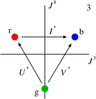
where the structure constants are given in App. B. For SU(3) we have two diagonal generators, usually chosen to be and , and six generators which define the ladder operators , , and , respectively. An explicit realization of (22) is, for example, given by the ’s as expressed in terms of Gell-Mann matrices in (14). This realization defines the fundamental representation of SU(3) illustrated in Fig. 3a. It is three-dimensional, and we have chosen to label the basis states by the colors blue (b), red (r), and green (g). The weight diagram depicted in Fig. 3a instructs us about the eigenvalues of the diagonal generators as well as the actions of the ladder operators on the basis states.
All other representations of SU(3) can be constructed by taking tensor products of reps. , which is again most conveniently accomplished using Young tableaux (see Fig. 4 for an example). The antisymmetrization over all boxes in the same column implies that we cannot have more than three boxes on top of each other. Each tableaux stands for an irreducible representation of SU(3), which can be uniquely labeled by their highest weight or Dynkin coordinates Cornwell84vol2 ; Georgi82 (see Fig. 5). For example, the fundamental representation has Dynkin coordinates (1,0). Note that all columns containing three boxes are superfluous, as the antisymmetrization of three colors yields only one state. In particular, the SU(3) singlet has Dynkin coordinates (0,0). In general, the dimension of a representation is given by . The labeling using bold numbers refers to the dimensions of the representations alone. Although this labeling is not unique, it will mostly be sufficient for our purposes. A representation and its conjugated counterpart are related to each other by interchange of their Dynkin coordinates.
IV.3 Examples of representations of SU(3)
We now consider some specific representations of SU(3) in detail. As starting point we use the fundamental representation spanned by the states , , and . The second three-dimensional representation is obtained by antisymmetrically coupling two reps. . The Dynkin coordinates of the rep. are (0,1), i.e., the reps. and are complex conjugate of each other. An explicit basis of the rep. is given by the colors yellow (y), cyan (c), and magenta (m),
| (23) | |||||
The weight diagram is shown in Fig. 3.b. The generators are given by (14) with replaced by , where ∗ denotes complex conjugation of the matrix elements Georgi82 . In particular, we find , , and .
The six-dimensional representation has Dynkin coordinates (2,0), and can hence be constructed by symmetrically coupling two reps. . The basis states of the rep. are shown in Fig. 6. The conjugate representation can be constructed by symmetrically coupling two reps. .
Let us now consider the tensor product . The weight diagram of the so-called adjoint representation is shown in Fig. 7. The states can be constructed starting from the highest weight state , yielding , , , and so on. This procedure yields two linearly independent states with . The representation can also be obtained by coupling of the reps. and , as can be seen from the Young tableaux in Fig. 4. On a more abstract level, the adjoint representation is the representation we obtain if we consider the generators themselves basis vectors. In the weight diagram shown in Fig. 7, the generators and correspond to the two states at the origin, whereas the ladder operators , , and correspond to the states at the six surrounding points. In the notation of Fig. 7, the singlet orthogonal to is given by .
The weight diagrams of four other representations relevant to our purposes below are shown in Figs. 8 to 10.
It is known that the physical properties of SU(2) spin chains crucially depend on whether on the lattice sites are integer or half-integer spins. A similar distinction can be made for SU(3) chains, as elaborated in Sec. X. The distinction integer or half-integer spin for SU(2) is replaced by a distinction between three families of irreducible representations of SU(3): either the number of boxes in the Young tableau is divisible by three without remainder (e.g. , , , ), with remainder one (e.g. , , , ), or with remainder two (e.g. , , , ).
While SU(2) has only one Casimir operator, SU(3) has two. The quadratic Casimir operator is defined as
| (24) |
where the ’s are the generators of the representation. As commutes with all generators it is proportional to the identity for any finite-dimensional irreducible representation. The eigenvalue in a representation with Dynkin coordinates is Cornwell84vol2
| (25) |
We have chosen the normalization in (24) according to the convention
which yields for the representation . Note that the quadratic Casimir operator cannot be used to distinguish between a representation and its conjugate. This distinction would require the cubic Casimir operator Cornwell84vol2 , which we will not need for any of the models we propose below.
V The trimer model (continued)
V.2 Verification of the model
We will now proceed with the verification of the trimer Hamiltonian (17). Since the spins on the individual sites transform under the fundamental representation , the SU(3) content of four sites is
| (26) |
i.e., we obtain representations , , and two non-equivalent 15-dimensional representations with Dynkin coordinates and , respectively. All these representations can be distinguished by their eigenvalues of the quadratic Casimir operator, which is given by if the four spins reside on the four neighboring lattice sites .
For the trimer states (11), the situation simplifies as we only have the two possibilities
which implies that the total SU(3) spin on four neighboring sites can only transform under representations or . The eigenvalues of the quadratic Casimir operator for these representations are and , respectively. The auxiliary operators
| (27) |
hence annihilate the trimer states for all values of , while they yield positive eigenvalues for or , i.e., all other states. Summing over all lattice sites yields (17). We have numerically confirmed by exact diagonalization of (17) for chains with and 12 lattice sites that the three states (12) are the only ground states.
Note that the representation content of five neighboring sites in the trimer chains is just the conjugate of the above, as
Since the quadratic Casimirs of conjugate representations have identical eigenvalues, , we can construct another parent Hamiltonian for the trimer states (12) by simply replacing with in (17). This Hamiltonian will have a different spectrum. In comparison to the four-site interaction Hamiltonian (17), however, it is more complicated while bearing no advantages. We will not consider it further.
V.3 Elementary excitations
(a)
(b)
Let us now turn to the low-lying excitations of (17). In analogy with the MG model, it is evident that the SU(3) spinon or “coloron” excitations correspond to domain walls between the degenerate ground states. For the trimer model, however, there are two different kinds of domain walls, as illustrated by:
| (28) | |||
| (29) |
The first domain wall (28) connects ground state to the left to ground state to the right, where is defined modulo 3 (see (12)), and consists of an individual SU(3) spin, which transforms under representation . The second domain wall (29) connects ground state with ground state . It consists of two antisymmetrically coupled spins on two neighboring sites, and hence transforms under representation . As we take momentum superpositions of the localized domain walls illustrated above, we expect one of them, but not both, to constitute an approximate eigenstate of the trimer model. The reason we do not expect both of them to yield a valid excitation is that they can decay into each other, i.e., if the rep. excitation is valid the rep. domain wall would decay into two rep. excitations, and vice versa. The question which of the two excitations is the valid one, i.e., whether the elementary excitations transform under or under SU(3) rotations, can be resolved through numerical studies. We will discuss the results of these studies now.
| mom | % | over- | ||
|---|---|---|---|---|
| exact | trial | off | lap | |
| 0 | 2.9735 | 4.5860 | 54.2 | 0.9221 |
| 1, 12 | 6.0345 | 10.2804 | 70.4 | 0.5845 |
| 2, 11 | 9.0164 | 17.2991 | 91.9 | 0.0 |
| 3, 10 | 6.6863 | 13.1536 | 96.7 | 0.0 |
| 4, 9 | 3.0896 | 5.0529 | 63.5 | 0.8864 |
| 5, 8 | 4.8744 | 7.5033 | 53.9 | 0.8625 |
| 6, 7 | 8.5618 | 16.6841 | 94.9 | 0.1095 |

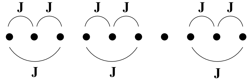
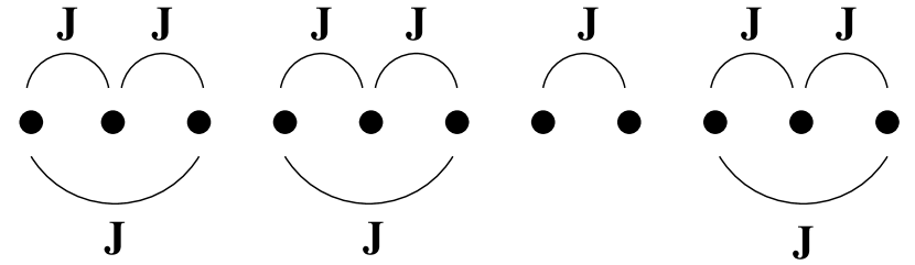
The rep. and the rep. trial states require chains with and sites, respectively; we chose and for our numerical studies. To create the localized domain walls (28) and (29), we numerically diagonalized auxiliary Hamiltonians with appropriate couplings, as illustrated in Fig. 11. From these localized excitations, we constructed momentum eigenstates by superposition, and compared them to the exact eigenstates of our model Hamiltonian (17) for chains with the same number of sites. The results are shown in Tab. 1 and Fig. 12 for the rep. trial state, and in Tab. 2 and Fig. 13 for the rep. trial state.
| mom | % | over- | ||
|---|---|---|---|---|
| exact | trial | off | lap | |
| 0 | 2.1013 | 2.3077 | 9.8 | 0.9953 |
| 1, 13 | 4.3677 | 4.8683 | 11.5 | 0.9864 |
| 2, 12 | 7.7322 | 8.7072 | 12.6 | 0.9716 |
| 3, 11 | 6.8964 | 7.7858 | 12.9 | 0.9696 |
| 4, 10 | 3.2244 | 3.5415 | 9.8 | 0.9934 |
| 5, 9 | 2.2494 | 2.4690 | 9.7 | 0.9950 |
| 6, 8 | 5.4903 | 6.1016 | 11.1 | 0.9827 |
| 7 | 7.4965 | 8.5714 | 14.3 | 0.9562 |

The numerical results clearly indicate that the rep. trial states (29) are valid approximations to the elementary excitations of the trimer chain, while the rep. trial states (28) are not. We deduce that the elementary excitations of the trimer chain (17) transform under , that is, under the representation conjugated to the original SU(3) spins localized at the sites of the chain. Using the language of colors, one may say that if a basis for the original spins is spanned by blue, red, and green, a basis for the excitations is spanned by the complementary colors yellow, cyan, and magenta. This result appears to be a general feature of SU(3) spin chains, as it was recently shown explicitly to hold for the Haldane–Shastry model as well bouwknegt-96npb345 ; schuricht-05epl987 ; schuricht-06prb235105 .
Note that the elementary excitations of the trimer chain are deconfined, meaning that the energy of two localized representation domain walls or colorons (29) does not depend on the distance between them. The reason is simply that domain walls connect one ground state with another, without introducing costly correlations in the region between the domain walls. In the case of the MG model and the trimer model introduced here, however, there is still an energy gap associated with the creation of each coloron, which is simply the energy cost associated with the domain wall.
In most of the remainder of this article, we will introduce a family of exactly soluble valence bond models for SU(3) chains of various spin representations of the SU(3) spins at each lattice site. To formulate these models, we will first review Schwinger bosons for both SU(2) and SU(3) and the AKLT model.
VI Schwinger Bosons
Schwinger bosons schwinger65proc ; Auerbach94 constitute a way to formulate spin- representations of an SU(2) algebra. The spin operators
| (30) |
are given in terms of boson creation and annihilation operators which obey the usual commutation relations
| (31) |
It is readily verified with (31) that , , and satisfy (19). The spin quantum number is given by half the number of bosons,
| (32) |
and the usual spin states (simultaneous eigenstates of and ) are given by
| (33) |
In particular, the spin- states are given by
| (34) |
i.e., and act just like the fermion creation operators and in this case. The difference shows up only when two (or more) creation operators act on the same site or orbital. The fermion operators create an antisymmetric or singlet configuration (in accordance with the Pauli principle),
| (35) |
while the Schwinger bosons create a totally symmetric or triplet (or higher spin if we create more than two bosons) configuration,
| (36) | |||||
The generalization to SU() proceeds without incident. We content ourselves here by writing the formalism out explicitly for SU(3). In analogy to (30), we write the SU(3) spin operators (14)
| (37) |
in terms of the boson annihilation and creation operators (blue), (red), and (green) satisfying
| (38) |
while all other commutators vanish. Again, it is readily verified with (38) that the operators satisfy (22). The basis states spanning the fundamental representation may in analogy to (34) be written using either fermion or boson creation operators:
| (39) |
We write this abbreviated
| (40) |
The fermion operators can be used to combine spins transforming under the fundamental representation antisymmetrically, and hence to construct the representations
| (41) |
The Schwinger bosons, by contrast, combine fundamental representations symmetrically, and hence yield representations labeled by Young tableaux in which the boxes are arranged in a horizontal row, like
| (42) |
where . Unfortunately, it is not possible to construct representations like
by simply taking products of anti-commuting or commuting creation or annihilation operators.
VII The AKLT model
Using the SU(2) Schwinger bosons introduced in the previous section, we may rewrite the Majumdar–Ghosh states (3) as
| (43) |
This formulation was used by Affleck, Kennedy, Lieb, and Tasaki affleck-88cmp477 ; affleck-87prl799 to propose a family of states for higher spin representations of SU(2). In particular, they showed that the valance bond solid (VBS) state
| (44) | |||||
is the exact zero-energy ground state of the spin-1 extended Heisenberg Hamiltonian
| (45) |
with periodic boundary conditions. Each term in the sum (45) projects onto the subspace in which the total spin of a pair of neighboring sites is . The Hamiltonian (45) thereby lifts all states except (44) to positive energies. The VBS state (44) is a generic paradigm as it shares all the symmetries, but in particular the Haldane spin gap haldane83pla464 ; haldane83prl1153 ; affleck89jpcm3047 , of the spin-1 Heisenberg chain. It even offers a particularly simple understanding of this gap, or of the linear confinement potential between spinons responsible for it, as illustrated by the cartoon:
Our understanding greiter02prb134443 ; greiter02prb054505 of the connection between the confinement force and the Haldane gap is that the confinement effectively imposes an oscillator potential for the relative motion of the spinons. We then interpret the zero-point energy of this oscillator as the Haldane gap in the excitation spectrum.
The AKLT state can also be written as a matrix product kluemper-91jpal955 ; kluemper-92zpb281 ; kluemper-93epl293 . We first rewrite the valence bonds
and then use the outer product to combine the two vectors at each site into a matrix
| (46) |
Assuming PBCs, (44) may then be written as the trace of the matrix product
| (47) |
In the following section, we will propose several exact models of VBSs for SU(3).
VIII SU(3) valence bond solids
To begin with, we use SU(3) Schwinger bosons introduced in Sec. VI to rewrite the trimer states (12) as
| (48) | |||||
where, as in (12), labels the three degenerate ground states, runs over the lattice sites subject to the constraint that is integer, and the sum extends over all six permutations of the three colors b, r, and g. This formulation can be used directly to construct VBSs for SU(3) spin chains with spins transforming under representations and on each site.
VIII.1 The representation VBS
We obtain a representations VBS from two trimer states by projecting the tensor product of two fundamental representations onto the symmetric subspace, i.e., onto the in the decomposition . Graphically, this is illustrated as follows:
| (49) |
This construction yields three linearly independent VBS states, as there are three ways to choose two different trimer states out of a total of three. These three VBS states are readily written out using (48),
| (50) |
for , 2, or 3. If we pick four neighboring sites on a chain with any of these states, the total SU(3) spin of those may contain the representations
or the representations
i.e., the total spin transforms under , , or , all of which are contained in the product
| (51) |
and hence possible for a representation spin chain in general. The corresponding Casimirs are given by , , and . This leads us to propose the parent Hamiltonian
| (52) |
with
| (53) |
Note that the operators , , are now given by matrices, as the Gell-Mann matrices only provide the generators (14) of the fundamental representation . Since the representations , , and possess the smallest Casimirs in the expansion (51), and hence also are positive semi-definite (i.e., have only non-negative eigenvalues). The three linearly independent states (50) are zero-energy eigenstates of (52).
To verify that these are the only ground states, we have numerically diagonalized (52) for and sites. For , we find zero-energy ground states at momenta (in units of with the lattice constant set to unity). Since the dimension of the Hilbert space required the use of a LANCZOS algorithm, we cannot be certain that there are no further ground states. We therefore diagonalized (52) for as well, where we were able to obtain the full spectrum. We obtained five zero energy ground states, two at momentum and one each at . One of the ground states at and the ground states constitute the space of momentum eigenstates obtained by Fourier transform of the space spanned by the three VBS states (50). The remaining two states at are the momentum eigenstates formed by superposition of the state
| (54) |
and the same translated by one lattice spacing. It is readily seen that these two states are likewise zero energy eigenstates of (52) for sites. The crucial difference, however, is that the VBS states (50) remain zero-energy eigenstates of (52) for all ’s divisible by three, while the equivalent of (54) for larger do not. We hence attribute these two additional ground states for to the finite size, and conclude that the three states (50) are the only zero-energy ground states of (52) for general ’s divisible by three.
Excitations of the VBS model are given by domain walls between two of the ground states (50). As in the trimer model, two distinct types of domain walls exist, which transform according to representations and :
| (55) |
It is not clear which excitation has the lower energy, and it appears likely that both of them are stable against decay. Let us first look at the rep. excitation. The four-site Hamiltonian (53) annihilates the state for all ’s except the four sites in the dashed box in (55), which contains the representations
| (56) |
i.e., the representations , twice, and with Casimirs , and , respectively, in addition to representations annihilated by . For the rep. excitation sketched on the right in (55), there are two sets of four neighboring sites not annihilated by as indicated by the dashed and the dotted box. Each set contains the representations
i.e., only the rep. in addition to representations annihilated by . For our parent Hamiltonian (52), it hence may well be that the rep. anti-coloron has the lower energy, but it is all but clear that the rep. has sufficiently higher energy to decay. For general representation spin chains, it may depend on the specifics of the model which excitation is lower in energy and whether the conjugate excitation decays or not.
Since the excitations of the rep. VBS chain are merely domain walls between different ground states, there is no confinement between them. We expect the generic antiferromagnetic rep. chain to be gapless, even though the model we proposed here has a gap associated with the energy cost of creating a domain wall.
VIII.2 The representation 10 VBS
Let us now turn to the VBS chain, which is a direct generalization of the AKLT chain to SU(3). By combining the three different trimer states (48) for symmetrically,
| (57) | |||||
we automatically project out the rep. in the decomposition generated on each lattice site by the three trimer chains. This construction yields a unique state, as illustrated:
| (58) |
In order to construct a parent Hamiltonian, note first that the total spin on two (neighboring) sites of a rep. chain is given by
| (59) |
On the other hand, the total spin of two neighboring sites for the VBS state can contain only the representations
| (60) |
as can be seen easily from the dashed box in the cartoon above. (Note that this result is independent of how many sites we include in the dashed box.) After the projection onto rep. on each lattice site, we find that only reps. and occur for the total spin of two neighboring sites for the VBS state. With the Casimirs and we obtain the parent Hamiltonian
| (61) |
the operators , , are now matrices, and we have used . is positive semi-definite and annihilates the VBS state (57). We assume that (57) is the only ground state of (61).
The Hamiltonian (61) provides the equivalent of the AKLT model affleck-87prl799 ; affleck-88cmp477 , whose unique ground state is constructed from dimer states by projection onto spin 1, for SU(3) spin chains. Note that as in the case of SU(2), it is sufficient to consider linear and quadratic powers of the total spin of only two neighboring sites. This is a general feature of the corresponding SU() models, as we will elaborate in the following section.
Since the VBS state (57) is unique, we cannot have domain walls connecting different ground states. We hence expect the coloron and anti-coloron excitations to be confined in pairs, as illustrated below. The state between the excitations is no longer annihilated by (61), as there are pairs of neighboring sites containing higher-dimensional representations, as indicated by the dotted box below. As the number of such pairs increases linearly with the distance between the excitation, the confinement potential depends linearly on this distance.
| (62) |
In principle, it would also be possible to create three colorons (or three anti-colorons) rather than a coloron–anti-coloron pair, but as all three excitations would feel strong confinement forces, we expect the coloron–anti-coloron pair to constitute the dominant low energy excitation. The confinement force between the pair induces a linear oscillator potential for the relative motion of the constituents. The zero-point energy of this oscillator gives rise to a Haldane-type energy gap (see greiter02prb134443 ; greiter02prb054505 for a similar discussion in the two-leg Heisenberg ladder), which is independent of the model specifics. We expect this gap to be a generic feature of rep. spin chains with short-range antiferromagnetic interactions.
VIII.3 The representation 8 VBS
To construct a representation VBS state, consider first a chain with alternating representations and on neighboring sites, which we combine into singlets. This can be done in two ways, yielding the two states
We then combine a – state with an identical one shifted by one lattice spacing. This yields representations at each site. The VBS state is obtained by projecting onto representation . Corresponding to the two – states illustrated above, we obtain two linearly independent VBS states, and , which may be visualized as
| (63) |
These states transform into each other under space reflection or color conjugation (interchange of and ).
It is convenient to formulate the corresponding state vectors as a matrix product. Taking (b,r,g) and (y,c,m) as bases for the reps. and , respectively, the singlet bonds in above can be written
| (64) |
We are hence led to consider matrices composed of the outer product of these vectors on each lattice site,
In the case of the AKLT model reviewed above, the Schwinger bosons take care of the projection automatically, and we can simply assemble these matrices into a product state. For the VBS, however, we need to enforce the projection explicitly. This is most elegantly accomplished using the Gell-Mann matrices, yielding the projected matrix
| (65) |
Here we have simply used the fact that the eight Gell-Mann matrices, supplemented by the unitary matrix, constitute a complete basis for the space of all complex matrices. By omitting the unit matrix in the expansion (65), we effectively project out the singlet state. Written out explicitly, we obtain
| (66) |
Assuming PBCs, the VBS state (illustrated in on the left (63)) is hence given by the trace of the matrix product
| (67) |
To obtain the state (illustrated on the right in (63)) we simply have to transpose the matrices in the product,
| (68) |
Let us now formulate a parent Hamiltonian for these states. If we consider two lattice sites on an SU(3) chain with a representation on each lattice site in general, we find the full SU(3) content
| (69) |
with , , and . On the other hand, for the VBS states only the representations can occur for the total spin of two neighboring sites, as the two sites always contain one singlet (see dashed box in (63) on the right above). With the Casimirs and for representations and , respectively, we construct the parent Hamiltonian
| (70) |
where the operators , , are now matrices, and we have used the Casimir on each site. is positive semi-definite, and annihilates the states and . We have numerically verified for chains with , 4, 5, and 6 lattice sites that and are the only ground states of (70).
Naively, one might assume the VBS model to support deconfined spinons or colorons, which correspond to domain walls between the two ground states and . A closer look at the domain walls, however, shows that this is highly unlikely, as each domain wall is a bound state of either two anti-colorons or two colorons, as illustrated below.
| (71) |
There is no reason to assume that the domain wall depicted above as two anti-colorons in fact corresponds to a single coloron, as it appears to be the case for the trimer chain. There we created a domain wall corresponding to a single coloron by removing one of the rep. spins from a trimer, leaving the remaining rep. spins coupled antisymmetrically as in the ground state. If we were to combine the two reps. into a rep. in (71), we would not reproduce a correlation present in the ground state, but enforce a new correlation. The correct interpretation of the domain wall between and is hence that of a bound state between two linearly confined anti-colorons. The origin of the confining potential is illustrated below.
| (72) |
As in the VBS, the confinement induces a linear oscillator potential for the relative motion of the anti-colorons. The zero-point energy of this oscillator corresponds to a Haldane-type gap in the spectrum. The ground state wave function of the oscillator is symmetric, and hence corresponds to a symmetric combination of , i.e., rep. . The antisymmetric combination corresponds to the first excited state of the oscillator, which we expect to cost more than twice the energy of the symmetric state greiter02prb054505 . This statement holds for the pair of colorons in (71) as well.

The domain walls, however, are not the only low energy excitations. In either of the ground states, we can create coloron–anti-coloron bound states, which make no reference to the other ground state, as illustrated below.
| (73) |
The oscillator model tells us again that the “symmetric” combination of , i.e., rep. , has the lowest energy, which we expect to be comparable, if not identical, to the energy required to create each of the domain walls above. The singlet will have an energy comparable to that of a domain wall transforming under either or . In any event, we expect the VBS model to display a Haldane gap due to coloron confinement.
The excitation spectrum of (70) for a chain with sites and PBCs is shown in Fig. 14. The spectrum shows that the lowest excitation transforms under rep. , as expected from (73), with a singlet and then another rep following at slightly higher energies. It is tempting to interpret those three levels as the lowest levels of the coloron–anti-coloron oscillator (73), but then there should be another singlet at a comparable spacing above. The fact that the spacings between these excitations are significantly smaller than the energy of the first exited state, however, would be consistent with such an interpretation, as the spinons in VBS models always have a local energy cost associated with their creation, which is specific to these models and not related to the universal Haldane gap stemming from confinement forces.
Most importantly, the spectrum provides strong evidence in favor of our assumption that the domain walls are not elementary excitations, but bound states of either two colorons or two anti-colorons, and hence that the lowest energy excitations of finite chains are coloron–anti-coloron bound states as illustrated in (73). The assumption is crucial for our conclusion that the model exhibits a Haldane gap. If the low energy sector of the model was determined by two deconfined domain walls, we would see a continuum of states in the spectrum, similar to the spectrum seen in spin chains of SU(2). The well defined low-energy modes in Fig. 14, however, look much more like the spinon–spinon bound state excitations seen in chains or two-leg Heisenberg ladders. In particular, if we assume that the individual domain walls transform under reps. and , we expect excitations transforming under the representations contained in to be approximately degenerate. Fig. 14 shows clearly that such a multiplet is not present a the lowest energies.
IX SU() models
In this section, we generalize three of the models proposed for SU(3) spin chains, the trimer model, the symmetric representation VBS, and the matrix product state VBS to the case of SU() spin chains.
IX.1 The -mer model
Consider an SU() spin chain with sites, where is a multiple of , with a spin transforming according to the fundamental representation of SU() at each lattice site,
| (74) |
where denotes a “flavor”, , and creates a fermion of flavor .
The SU() generators at site are in analogy to (5) and (14) defined as
| (75) |
where the denote the SU() Gell-Mann matrices macfarlane-68cmp77 . The generators are normalized through the eigenvalue the quadratic Casimir operator takes in the adjoint representation, .
To determine the eigenvalues of the quadratic Casimir for general representations of SU(), a significant amount of representation theory is required Humphreys87 . We content ourselves here by providing the formulas up to in App. C.
In analogy to the trimer states (12), we construct the -mer states of an SU() spin chain by combining sets of neighboring spins into a singlet,
| (76) |
where labels the degenerate ground states, and runs over the lattice sites subject to the constraint that is integer. The sum extends over all permutations of the flavors .
In order to identify a parent Hamiltonian, consider the total SU() spin on neighboring sites for the -mer states. Following the rules of combining representations labeled by Young tableaux (see e.g. Cornwell84vol2 ; Georgi82 ), it is not difficult to see that the total spin will only contain representations given by tableaux with boxes and two columns, i.e., tableaux of the form
with . The eigenvalues of the quadratic Casimir operator for these representations are
| (77) |
An educated guess for a parent Hamiltonian for the -mer chain hence appears to be
| (78) |
with
| (79) |
where denotes the floor function, i.e., is the largest integer , and we use the notation introduced in (16).
This construction yields the MG model majumdar-69jmp1399 for SU(2), the trimer model (17) for SU(3), and a valid parent Hamiltonian for the four degenerate 4-mer states for SU(4). For , however, the decomposition of the tensor product contains irreducible representations corresponding to Young tableaux with more than two columns, whose Casimirs are equal or smaller than a number of Casimirs included in the list , . If the Casimir of such an “undesired” representation not included in the list is smaller than an odd number of Casimirs included in the list, we obtain negative eigenvalues for , and it is not a priori clear any more that the Hamiltonian (78) is positive semi-definite. An obvious cure to this problem is to write
| (80) |
with as in (79). This does, however, not cure potential problems arising from undesired representations which share the eigenvalues of the Casimir with one of the representations from the list, as it happens to be the case for . The Hamiltonian (80) likewise annihilates these representations, giving rise to a remote possibility that the -mer states (76) are not the only ground states of (80). The potential relevance of these problems has to be investigated for each separately.
IX.2 The representation VBS
As a generalization of the AKLT model for SU(2) and the VBS model for SU(3) discussed above, we now consider a VBS for an SU() chain of spins transforming under the symmetric representation
where each , , is an SU() Schwinger boson. The VBS state is obtained by combining -mer states (76), one for each , in that the total spin on each lattice site is projected onto the symmetric representation . This yields
| (81) |
Let us now construct a parent Hamiltonian for the symmetric VBS (81). The total SU() spin of two neighboring sites of a representation spin chain in general contains all the representations corresponding to Young tableaux with boxes and at most two rows, i.e., all tableaux of the form
The eigenvalues of the quadratic Casimir operator for these representations are given by
| (82) |
On the other hand, the total SU() spin of two neighboring sites of the representation VBS (81) has to be contained in the product
| (83) |
As we project the spin on each lattice site onto the representation , only two these representations remain:
The eigenvalues of the quadratic Casimir operator are given by and , respectively. Hence, using , we obtain the parent Hamiltonian
| (84) |
Since for and is a strictly increasing function of , the Hamiltonian (84) is positive semi-definite. For , we recover the AKLT model (45); for , we recover the VBS model (61).
IX.3 An example of a matrix product state
In principle, a matrix product VBS can be formulated on all SU() chains with spins transforming under the symmetric combination of any representation and its conjugate representation . Unless the rep. is self-conjugate, we obtain two inequivalent states, which transform into each other under space reflection. The construction of these is analogous to the VBS introduced above, and likewise best illustrated as
| (85) |
The thick lines indicate that we combine pairs of neighboring representations and into singlets. On each lattice site, we project onto the symmetric combination of and , as indicated. By “symmetric combination” we mean that if representations and of SU() have Dynkin coordinates and , respectively, we combine them into the representation with Dynkin coordinates . In other words, we align the columns of both tableaux horizontally, and hence obtain a tableau with twice the width, without ever adding a single box vertically to a column of the tableaux we started with. The states (85) we obtain are translationally invariant and we expect the parent Hamiltonians to involve nearest-neighbor interactions only.
In this subsection, we will formulate the simplest SU() model of this general family. We take to be the representation formed by antisymmetrically combining fundamental representations,
which implies that we consider a model with the representation
corresponding to a Young tableaux with a column with boxes
to the left of a column with boxes at each lattice site:
The construction of the parent Hamiltonian is similar to the -mer model above. The total spin on two neighboring lattice sites can only assume representations contained in , i.e., representations corresponding to tableaux of the form
with . The eigenvalues of the quadratic Casimir operator for these representations are
| (86) |
The obvious proposal for a parent Hamiltonian is hence
| (87) |
where denotes again the floor function. This Hamiltonian singles out the matrix product state (85) as unique ground states for , but suffers from the same shortcomings as (78) with (79) for .
X Spinon confinement and the Haldane gap
X.1 The Affleck–Lieb theorem
For the generic SU(2) spin chain, Haldane haldane83pla464 ; haldane83prl1153 identified the O(3) nonlinear sigma model as the effective low energy field theory of SU(2) spin chains, and argued that chains with integer spin possess a gap in the excitation spectrum, while a topological term renders half-integer spin chains gapless affleck90proc ; Fradkin91 . The exact models for SU(2) spin chains we reviewed above, the MG and the AKLT chain, serve a paradigms to illustrate the general principle. Unfortunately, the effective field theory description of Haldane yielding the distinction between gapless half integer spin chains with deconfined spinons and gapped integer spin chains with confined spinons cannot be directly generalized to SU() chains, as there is no direct equivalent of the CP1 representation used in Haldane’s analysis.
Nonetheless, there is a rigorous and rather general result for antiferromagnetic chains of SU() spins transforming under a representation corresponding to a Young tableau with a number of boxes not divisible by : Affleck and Lieb affleck-86lmp57 showed that if the ground state is non-degenerate, and the Hamiltonian consists nearest-neighbor interactions only, than the gap in the excitation spectrum vanishes as (where is the number of sites) in the thermodynamic limit. This result is fully consistent with the picture suggested by the models introduced above. Like the MG model, the trimer model and the representation VBS have degenerate ground states and interactions which extend beyond the nearest neighbor, which implies that the theorem is not directly applicable.
On physical grounds, however, the statement that a given model is gapless (i.e., the excitation gap vanishes in the thermodynamic limit) implies that the spinons are deconfined. The reason is simply that if there was a confinement force between them, the zero-point energy associated with the quantum mechanical oscillator of the relative motion between the spinons would inevitably yield an energy gap. The MG, the trimer and the VBS model constitute pedagogically valuable paradigms of deconfined spinons. Since the excitations in these models are literally domain walls between different ground states, no long-range forces can exist between them.
X.2 A general criterion for spinon confinement
More importantly, however, the exact models we introduced above provide information about the models of SU() spin chains with representations corresponding to Young tableaux with a number of boxes divisible by , i.e., models for which the Affleck–Lieb theorem is not applicable. We have studied two SU(3) models belonging to this family in Sec. VIII, the rep. VBS and the rep. VBS, and found that both have confined spinons or colorons and hence display a Haldane-type gap in the spectrum.
In this section, we will argue that models of antiferromagnetic chains of SU() spins transforming under a representation corresponding to a Young tableau consisting of a number of boxes divisible by generally possess a Haldane-type gap due to spinon confinement forces.
We should caution immediately that our argument is based on several assumptions, which we consider reasonable, but which we are ultimately unable to prove.
The first, and also the most crucial, is the assumption that the question of whether a given model supports free spinon excitations can be resolved through study of the corresponding VBS state. This assumption definitely holds for SU(2) spin chains, where the MG model for indicates that the spinons are free, while the AKLT model for serves as a paradigm for spinon confinement and hence the Haldane gap. The general conclusions we derived from our studies of the SU(3) VBSs above rely on this assumption. The numerical results we reported on the rep. VBS provide evidence that this assumption holds at least for this model.
Let us consider an SU() spin chain with spins transforming under a representation corresponding to Young tableau consisting of columns with boxes each,
| (88) |
with a total number of boxes
divisible by . We denote the Dynkin coordinates of this representation by , which implies
Note that this representation is, by definition, given by the maximally symmetric component of the tensor product of the individual columns,
| (89) |
For convenience, we denote the dimensional representation in this subsection as .
Since is divisible by , it will always be possible to obtain a singlet from the complete sequence of representations by combining them antisymmetrically. To be precise, when we write that we combine representations and antisymmetrically, we mean we obtain a new representation by stacking the two columns with and boxes on top of each other if , and a new representation if . In equations, we write this as
| (90) |
Following the notation used above, we indicate the antisymmetric combination of representations by a line connecting them. In particular, we depict the singlet formed by combining on different lattice sites as
| (91) |
The understanding here is that we combine them in the order indicated by the line, i.e., in (91) we first combine and , then we combine the result with , and so on. Depending on the order of the representations on the line, we obtain different, but not necessarily orthogonal, singlets. We assume that it is irrelevant whether we combine the representations starting from the left or from the right of the line, as the resulting state will not depend on it.
In general, it will be possible to construct a number of singlets out of various combinations of the ’s, one for each block of ’s for which the values of add up to as we combine the representation in the order described above. In this case, we will be able to construct one VBS for each singlet, and subsequently combine them at each site symmetrically to obtain the desired representation (88). The argument for spinon confinement we construct below will hold for each of the individual VBSs, and hence for the combined VBS as well. It is hence sufficient for our purposes to consider situations where the entire sequence is needed to construct a singlet.
A possible VBS “ground state” for a representation corresponding to a Young tableau with columns is depicted below.
| (92) |
In general, there are as many inequivalent VBS “ground states” as there are inequivalent ways to order the representations , i.e., the number of inequivalent VBS “ground states” is given by
To give an example, the following VBS
| (93) |
is inequivalent to the one above if and only if . Note that all these VBS “ground states” states are translationally invariant. We expect some of these states, but not all of them, degenerate in energy for the appropriate parent Hamiltonian, and have accordingly written “ground states” in quotation marks. For example, if we form a SU(4) VBS with representation , the combination
might yield a state with a lower energy for the appropriate Hamiltonian than the state formed by combining
Simple examples where we have only two inequivalent VBS ground states are provided by the matrix product states discussed in Secs. VIII.3 and IX.3.
We will now argue that the elementary excitations of the corresponding VBS models are always confined. To this end, we first observe that any domain wall between translationally invariant “ground states” consists of a total of representations ( integer). To illustrate this, consider a domain wall between the “ground states” depicted in (93) and (92):
In the example, the domain wall consists of reps. , , , and . If the translationally invariant states on both sites are true ground states, the domain wall is likely to correspond to two elementary excitations: a rep. spinon consisting of an antisymmetric combination of a , a , and a , as indicated by the line in the drawing, and another rep. spinon. The reason we assume that , , and form a rep. is simply that this combination is present in both ground states on either side, and hence bound to be the energetically most favorable combination. The second , however, is not part of this elementary excitation, as combining it antisymmetrically with the others (i.e., the ) would induce correlations which are not present in the ground state. We hence conclude that the second is an elementary excitation as well. The domain wall depicted above consists of a spinon transforming under rep. and an anti-spinon transforming under rep. .
The next step in our argument is to notice that the spinon and the complementary particle created simultaneously which may either be its anti-particle or some other spinon, are confined through a linear potential. To see this, we pull them apart and look at the state inbetween (color online):
| (94) |
The state between spinon and anti-spinon is not translationally invariant. In the example, the unit cell of this state is depicted in red and consists of two regular bonds with three “singlet lines” between the sites, one stronger bond with four lines (which cross in the cartoon), and one weaker bond with only two lines. If we assume that the two states (93) and (92) on both sides are true ground states, it is clear that the irregularities in the strength of the bond correlations will cause the state between the spinon and anti-spinon to have a higher energy than either of them. This additional energy cost will induce a linear confinement potential between the spinons, and hence a linear oscillator potential for the relative motion of the particles. As in the models studied above, the Haldane gap corresponds to the zero-point energy of this oscillator.
If one of the “ground states” to the left or to the right of the domain wall is not a true ground state, but a translationally invariant state corresponding to a higher energy than the ground state, there will be a confining force between this domain wall and another domain wall which transforms the intermediate “ground state” with a higher energy back into a true ground state. This force will be sufficient to account for a Haldane gap, regardless of the strength or existence of a confinement force between the constituent particles of each domain wall.
The lowest-lying excitations of a representation spin chain, however, will in general not be domain walls, but spinons created by breaking up one of the singlets (91) in a ground state. This is illustrated below for the ground state (92):
In the example, we have created a spinon transforming under rep. and its anti-particle, a spinon transforming under rep. . This is, however, irrelevant to the argument—we may break the singlet in any way we like. The important feature is that we obtain, by construction, at least two excitations, and that these are confined. In our specific example, the confining potential is equivalent to the confining potential in (94) above (color online):
We leave it to the reader to convince him- or herself that the conclusions regarding confinement drawn from the simple examples studied here hold in general.
X.3 Models with confinement through interactions extending beyond nearest neighbors
Let us briefly summarize the results obtained. The SU() models we have studied so far fall into two categories. The models belonging to the first—the trimer chain, the VBS, and the -mer chain—have degenerate ground states, which break translational invariance up to translations by lattice spacings. The Young tableaux describing the representations of SU() at each site consist of a number of boxes which is smaller than , and hence obviously not divisible by . The models support deconfined spinon excitations, and hence do not possess a Haldane gap in the spectrum. The Hamiltonians of these models require interactions between neighboring sites along the chain. Even though the Affleck–Lieb theorem is not directly applicable to the models we constructed above, it is applicable to SU() spin chains with spins transforming under the same representations. Like the VBS models, the theorem suggests that there is no Haldane gap in this family of models.
The models belonging to the second category—the VBS, the VBS, the representation VBS, and the - matrix product state—have translationally invariant ground states. The ground states are unique for some models, like the and the VBS, and degenerate for others, like the VBS. The Young tableaux describing the representations of SU() at each site consist of a number of boxes which is divisible by . The Affleck–Lieb theorem is not applicable to models of this category. The spinon excitations for this category of models are subject to confinement forces, which give rise to a Haldane gap. The parent Hamiltonians for these models require interactions between nearest-neighbor sites only.
At first glance, this classification might appear complete. Further possibilities arise, however, in SU() spin chains where number of boxes the Young tableau consists of and have a common divisor different from , which obviously requires that is not a prime number. In this case, it is possible to construct VBS models in which the ground state breaks translational invariance only up to translations by lattice spacings, where denotes the largest common divisor of and such that . This implies that the ground state of the appropriate, translationally invariant Hamiltonian will be -fold degenerate. In the examples we will elaborate on below, the parent Hamiltonians for these models require interactions between sites, a feature we conjecture to hold in general. The spinon excitations of these models are confined, even though the Affleck–Lieb theorem states that the nearest-neighbor Heisenberg chain of SU() spins transforming under these representations is gapless. (We implicitly assume here that the ground states of the SU() nearest-neighbor Heisenberg chains are non-degenerate.) Let us illustrate the general features of this third category of models with a few simple examples.
(1) Consider an SU(4) chain with spins transforming under the 10-dimensional representation
Following the construction principle of the VBS of SU(3), we find that the two degenerate VBS states illustrated through
| (95) |
are exact zero-energy ground states of
| (96) |
which contains next-nearest neighbor interactions.
The example illustrates the general rule stated above. The largest common divisor of and is . This implies and hence two degenerate VBS states which break translational invariance up to translations by two lattice spacings. The parent Hamiltonian requires interaction between three neighboring sites.
According to the Affleck–Lieb theorem, models of antiferromagnetic SU(4) chains of representation with nearest-neighbor Heisenberg interactions and non-degenerate ground states are gapless in the thermodynamic limit, which implies that the spinons are deconfined. In all the models we have studied in previous sections, the conclusions drawn from the Affleck–Lieb theorem were consistent with those drawn from our exact models. For the present model, however, they are not consistent.
Specifically, we strongly conjecture that the spinons in the VBS are confined. This conjecture is based on the reasonable assumption that the elementary excitations of the model transform as either the fundamental representation of SU(4) or its conjugate representation . This assumption implies that a single domain wall in one of the -mer chains used to construct the VBS state (95) shifts this chain by one lattice spacing. If we assume a ground state to the left of the spinon, the state on to the right will have a higher energy for the next-nearest neighbor Hamiltonian (96), as illustrated below.
| (97) |
To recover the ground state, a second domain wall is required nearby, which is bound to the first by a linear potential.
Our conclusion is not in contradiction with the rigorous result of Affleck and Lieb, as they explicitly restrict themselves to models with nearest-neighbor interactions. If we had only nearest-neighbor interactions, the energy expectation value in the region between the domain walls would not be higher than in the ground state, as one can see easily from the cartoon above—the sequence of alternating links would merely shift from (strong, weak, strong, weak) to (strong, strong, weak, weak).
(2) The situation is similar for an SU(6) chain with spins transforming under the 56-dimensional representation
With and , we have again . Accordingly, we find that the two VBS states illustrated through
| (98) |
are exact ground states of a parent Hamiltonian containing up to next-nearest-neighbor interactions only, and that the spinon excitations are confined.
(3) As a third example, consider an SU(6) spin chain with spins transforming under the 21-dimensional representation
This implies . We find that the three VBS states illustrated by
| (99) |
are exact ground states of a parent Hamiltonian involving the quadratic Casimir of total spin of four neighboring sites,
| (100) |
with
| (101) |
These VBS states break translational symmetry only up to translations by three lattice spacings. The spinons of this model are again confined through a linear potential, as illustrated below.
| (102) |
The conclusions we have drawn for this VBS model rest on the assumption that the quadratic Casimirs of the representations contained in the tensor product shown in the dashed box in (99) as well as in the tensor product one obtains if one shifts this box by one lattice spacing to the left or to the right are smaller than the largest Casimir contained in the tensor product shown in the dotted box in (102). We have verified the validity of this assumption for the (2,0,0,0,0) VBS model we considered here, but not shown it to hold for similar models with larger or .
(4) Finally, consider an SU(6) spin chain with spins transforming under the 70-dimensional representation
Thus we have once again . In a notation similar to the one introduced for the VBS,
the two degenerate VBSs are illustrated by
| (103) |
are exact ground states of a parent Hamiltonian involving the quadratic Casimir of the total spin of three neighboring sites,
| (104) |
with
| (105) |
The states (103) are not the only VBSs one can form. Other possibilities like
or
however, contain additional representations for the total SU(6) spin of three neighboring sites, and are hence expected to possess higher energies.
Spinon excitations transforming under the 6-dimensional rep. are linearly confined to spinons transforming under the 15-dimensional rep. :
| (106) |
The VBS configuration we have drawn between the two spinons in (106) constitutes just one of several possibilities. We expect, however, that this possibility corresponds to the lowest energy among them for the Hamiltonian (104). This concludes our list of examples.
The models introduced in this subsection are interesting in that they provide us with examples where spinon confinement, and with the confinement the existence of a Haldane gap, is caused by interactions extending beyond nearest neighbors. The conclusion drawn from the Affleck–Lieb theorem for SU() models with spins transforming under representations we have labeled here as the “third category” hence appear to hold for models with nearest-neighbor interactions only, to which the theorem is applicable. For these models, the theorem states that the spectrum is gapless, which according to our understanding implies that the models support deconfined spinon excitations. The examples we have studied, by contrast, suggest that models with longer-ranged interactions belonging to this category exhibit confinement forces between the spinon excitations and hence possess a Haldane gap.
It is worth noting that even though in the examples we elaborated here , we expect our conclusions to hold for models with as well. To see this, let be an integer such that . We can now construct a first VBS with spinon confinement using boxes of the Young tableau and combine it with a second by projection on each side with a second VBS constructed from the remaining boxes. Since the spinons of the first VBS are always confined and hence gapped, the final VBS will support deconfined spinons if and only if the second VBS will support them, which in turn will depend on the largest common divisor of and as well as the range of the interaction. Since the largest common divisor of and is equal to , there is no need to think in terms of and . The conclusions regarding confinement and the Haldane gap will not depend on the distinction between and .
X.4 The different categories of models
In this section, we used the rules emerging from the numerous examples we studied to argue that models of SU() spin chains in general fall into three categories. The classification depends on the number of boxes the Young tableau corresponding to the representation of the individual spins consists off, as follows:
-
1.
If and have no common divisor, the models will support free spin excitations and hence not exhibit a Haldane gap.
The general reasoning here is simply that the VBS states in this category break translational invariance up to translations by lattice spacings, and that there are (at least) degenerate VBS ground states to each model. Spinons transforming under representations of Young tableaux with an arbitrary number of boxes can be accommodated in domain walls between these different ground states. Consequently, the spinons are deconfined.
-
2.
If is divisible by , the general argument we have constructed in Sec. X.2 indicates that the model will exhibit spinon confinement and hence a Haldane gap.
-
3.
If and have a common divisor different from , the examples studied in Sec. X.3 suggest that the question of whether the spinons are confined or not depends on the details of the interactions. If is the largest common divisor of and , interactions ranging to the -th neighbor were required for spinon confinement in the models we studied. The Affleck-Lieb theorem affleck-86lmp57 , on the other hand, tells us that SU() chains with nearest-neighbor Heisenberg interactions belonging to this category are gapless if the ground states are non-degenerate.
Note that the second category is really just the special case of the third: with , nearest-neighbor interactions are already sufficient for spinon confinement and a Haldane gap.
The conclusion that interactions ranging to the -th neighbor are required for spinon confinement and a Haldane gap, however, is not universally valid. A counter-example is provided by the extended VBSs (XVBSs) introduced by Affleck, Arovas, Marston, and Rabson affleck-91npb467 . In this model, each site effectively takes the role of two neighboring sites when a VBS is constructed, and nearest-neighbor interactions are already sufficient to cause spinon confinement. We briefly review this model in the following subsection.
X.5 A counter-example: the SU(4) representation extended VBS
In an article devoted to quantum antiferromagnets with spins transforming under the self-conjugate representations of SU(), Affleck et al. affleck-91npb467 introduced an extended VBS for the six-dimensional SU(4) representation . This representation is, with regard to the number of boxes the corresponding Young tableau consists of, not distinguishable from the symmetric representation considered in Sec. X.3, as both tableaux consist of two boxes:
| (107) |
Since the two boxes are combined antisymmetrically for rep. , a VBS constructed along the lines of Sec. X.3 would no longer provide a paradigm for antiferromagnetic spin chains of the corresponding representation in general. Affleck et al. affleck-91npb467 have constructed an extended VBS, which is illustrated in the following cartoon:
| (108) |
Here each small circle represents a fundamental representation of SU(4) (a box in the Young tableau), and each large circle a lattice site. The lines connecting four dots indicate that these four fundamental representations are combined into an SU(4) singlet. The total spin of two neighboring sites in this state may assume the representations
| (109) |
while combining two reps. on neighboring sites in general yields
| (110) |
To construct a parent Hamiltonian for the XVBS (108), it is hence sufficient to sum over projectors onto rep. on all pairs of neighboring sites. Using our conventions (Affleck et al. affleck-91npb467 have normalized the eigenvalues of the quadratic Casimir operator to ), the parent Hamiltonian takes the form
| (111) |
where the operators , , are given by matrices. Note that the ground state is two fold degenerate, as it breaks translational symmetry modulo translations by two lattice spacings.
We conjecture that the lowest lying excitation is a bound state consisting of two fundamental reps , which most likely are combined antisymmetrically into a rep. :
The SU(4) rep. XVBS provides us with an example where a nearest-neighbor Hamiltonian is sufficient to induce spinon confinement and a Haldane gap, even though the largest common divisor of and is , i.e., interactions including neighbors would be required following the rules derived from the examples in Sec. X.3. The reason for this discrepancy is that in the XVBS model considered here, each site effectively takes the role of two neighboring sites. Affleck et al. affleck-91npb467 ; marston-89prb11538 conjecture that the ground state of the SU(4) rep. nearest-neighbor Heisenberg model is, like the XVBS reviewed here, two-fold degenerate, which implies that the Affleck-Lieb theorem is not applicable.
This example is valuable in showing that it is advisable to explicitly construct the VBS for a given representation of SU() in order to verify the applicability of the general rules motivated above.
XI Conclusion
In the first part of this article, we have formulated several exact models of SU(3) spin chains. We introduced a trimer model and presented evidence that the elementary excitations of the model transform under the SU(3) representations conjugate to the representation of the original spin on the chain. We then introduced three SU(3) valence bond solid chains with spins transforming under representations , , and , respectively. We argued that of these four models, the coloron excitations are confined only in the and the VBS models, and that only those models with confined spinons exhibit a Haldane gap. We subsequently generalized three of our models to SU(), and investigated again which models exhibit spinon confinement.
Finally, we used the rules emerging from the numerous examples we studied to argue that models of SU() spin chains in general fall into three categories with regard to spinon confinement and the Haldane gap. These are summarized in the previous subsection. The results rely crucially on the assumption that the conclusions we obtained for the VBS models we studied are of general validity. This assumption certainly holds for the corresponding SU(2) models, and appears reasonable on physical grounds. Ultimately, however, it is only an assumption, or at best a hypotheses.
On a broader perspective, we believe that the models we have studied provide further indication that SU() spin chains are an equally rich and rewarding subject of study as SU(2) spin chains have been since Bethe.
ACKNOWLEDGMENTS
We would like to thank Peter Zoller and Peter Wölfle, but especially Dirk Schuricht and Ronny Thomale for many highly inspiring discussions of various aspects of this work. We further wish to thank Dirk Schuricht for valuable suggestions on the manuscript. One of us (SR) was supported by a Ph.D. scholarship of the Cusanuswerk.
Appendix A A proposal for an experimental realization of SU(3) spin chains in an optical lattice
In this appendix, we wish to describe a proposal for an experimental realization of SU(3) spin chains. The most eligible candidate for such experiments are ultra-cold gases in optical lattices. Recently, these systems have become an interesting playground for the realization of various problems of condensed matter physics, such as the phase transition from a superfluid to a Mott insulator Jaksch-98prl3108 ; Greiner-02n39 , the fermionic Hubbard model Honerkamp-04prl170403 ; Honerkamp-04prb094521 ; rapp-06cm0607138 , and SU(2) spin chains Duan-03prl090402 ; Garcia-04prl250405 . In particular, the Hamiltonians for spin lattice models may be engineered with polar molecules stored in optical lattices, where the spin is represented by a single-valence electron of a heteronuclear molecule micheli-06np341 ; brennen-06qp0612180 .
In a most naive approach, one might expect to realize an SU(3) spin (at a site in an optical lattice) by using atoms with three internal states, like an atom with spin . If we now were to interpret the state as SU(3) spin “blue”, the state as ”red”, and the state as “green”, however, the SU(3) spin would not be conserved. The SU(2) algebra would allow for the process , which in SU(3) language corresponds to the forbidden process .
A more sophisticated approach is hence required. One way to obtain a system with three internal states in which the number of particles in each state (i.e., of each color) is conserved is to manipulate an atomic system with total angular momentum (where includes the internal spin of the electrons, the orbital angular momentum, and the spin of the nucleus) to simulate an SU(3) spin. The important feature here is that the atoms have four internal states, corresponding to . For such atoms, one has to suppress the occupation of one of the “middle” states, say the state, by effectively lifting it to a higher energy while keeping the other states approximately degenerate. This can be accomplished through a combination of an external magnetic field and two carefully tuned lasers, which effectively push down the energies of the and the states by coupling these states to states of (say) the energetically higher multiplet (see Fig. 15).
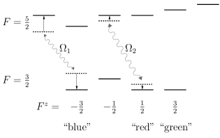
At sufficiently low temperatures, we are hence left with a system with three internal states , which we may identify with the colors “blue”, “red”, and “green” of an SU(3) spin. In leading order, the number of particles of each color is now conserved, as required by SU(3) symmetry. For example, conservation of forbids processes in which a “blue” and a “green” particle turn into two “red” ones, . Higher order processes of the kind are still possible, but negligible if the experiment is conducted at sufficiently short time scales.
If one places fermionic atoms with an artificial SU(3) spin engineered along the lines of this or a related proposal in an optical lattice and allows for a weak hopping of the atoms on the lattice, one has developed an experimental realization of an SU(3) Hubbard model. If the energy cost of having two atoms on the same lattice site is significantly larger than the hopping , and the density is one atom per site, the system will effectively constitute an SU(3) antiferromagnet. The dimension of this antiferromagnet will depend on the optical lattice, which can be one-, two-, or three-dimensional.
In principle, the above proposal can be generalized to SU(), even though the experimental obstacles are likely to grow “exponentially” with . Besides, it is far from clear that such an endeavor is worthwhile, as all the non-trivial properties of SU() are already present in SU(3) chains (while SU(2) constitutes a special case).
Appendix B Gell-Mann matrices
The Gell-Mann matrices are given by Cornwell84vol2 ; Georgi82
They are normalized as and satisfy the commutation relations The structure constants are totally antisymmetric and obey Jacobi’s identity
Explicitly, the non-vanishing structure constants are given by ,
,
, and 45 others obtained by permutations of
the indices.
Appendix C Eigenvalues of the quadratic Casimir operator
The eigenvalues of the quadratic Casimir operator for representations of SU() up to are given by:
The general method to obtain these and further eigenvalues for requires a discussion of representation theory Humphreys87 at a level which is beyond the scope of this article.
The dimensionality of a representation is determined by the so-called Hook formula Cornwell84vol2
| (112) |
where for . In particular, it yields for :
References
- (1) H. Bethe, Z. Phys. 71, 205 (1931), translated in D. C. Mattis, ed., The Many-Body Problem (World Scientific, Singapore, 1993).
- (2) C. N. Yang, Phys. Rev. Lett. 19, 1312 (1967).
- (3) R. J. Baxter, Exactly Solved Models in Statistical Mechanics (Academic Press, London, 1990).
- (4) V. E. Korepin, N. M. Bogoliubov, and A. G. Izergin, Quantum Inverse Scattering Method and Correlation Functions (Cambridge University Press, Cambridge, 1997).
- (5) L. D. Faddeev and L. A. Takhtajan, Phys. Lett. A 85, 375 (1981).
- (6) R. B. Laughlin, Phys. Rev. Lett. 50, 1395 (1983).
- (7) Quantum Hall Effect, edited by M. Stone (World Scientific, Singapur, 1992).
- (8) F. D. M. Haldane, Phys. Lett. A 93, 464 (1983).
- (9) F. D. M. Haldane, Phys. Rev. Lett. 50, 1153 (1983).
- (10) I. Affleck, in Fields, strings and critical phenomena, Vol. XLIX of Les Houches lectures, edited by E. Brézin and J. Zinn-Justin (Elsevier, Amsterdam, 1990).
- (11) E. Fradkin, Field Theories of Condensed Matter Systems, No. 82 in Frontiers in Physics (Westview Press, Bouler, 1991).
- (12) A. O. Gogolin, A. A. Nersesyan, and A. M. Tsvelik, Bosonization and Strongly Correlated Systems (Cambridge University Press, Cambridge, 1998).
- (13) T. Giamarchi, Quantum Physics in One Dimension (Oxford University Press, Oxford, 2004).
- (14) C. K. Majumdar and D. K. Ghosh, J. Math. Phys. 10, 1399 (1969).
- (15) I. Affleck, T. Kennedy, E. H. Lieb, and H. Tasaki, Phys. Rev. Lett. 59, 799 (1987).
- (16) I. Affleck, T. Kennedy, E. H. Lieb, and H. Tasaki, Commun. Math. Phys. 115, 477 (1988).
- (17) F. D. M. Haldane, Phys. Rev. Lett. 60, 635 (1988).
- (18) B. S. Shastry, Phys. Rev. Lett. 60, 639 (1988).
- (19) F. D. M. Haldane, Phys. Rev. Lett. 66, 1529 (1991).
- (20) F. D. M. Haldane, Z. N. C. Ha, J. C. Talstra, D. Bernard, and V. Pasquier, Phys. Rev. Lett. 69, 2021 (1992).
- (21) F. D. M. Haldane, Phys. Rev. Lett. 67, 937 (1991).
- (22) Z. N. C. Ha and F. D. M. Haldane, Phys. Rev. B 47, 12459 (1993).
- (23) F. H. L. Eßler, Phys. Rev. B 51, 13357 (1995).
- (24) M. Greiter and D. Schuricht, Phys. Rev. B 71, 224424 (2005).
- (25) M. Greiter, Statistical Phases and Momentum Spacings for One-Dimensional Anyons, submitted to Phys. Rev. Lett.
- (26) M. Greiter and D. Schuricht, Many-spinon states and the secret significance of Young tableaux, submitted to Phys. Rev. Lett.
- (27) N. Kawakami, Phys. Rev. B 46, 1005 (1992).
- (28) N. Kawakami, Phys. Rev. B 46, R3191 (1992).
- (29) Z. N. C. Ha and F. D. M. Haldane, Phys. Rev. B 46, 9359 (1992).
- (30) P. Bouwknegt and K. Schoutens, Nucl. Phys. B 482, 345 (1996).
- (31) D. Schuricht and M. Greiter, Europhys. Lett. 71, 987 (2005).
- (32) D. Schuricht and M. Greiter, Phys. Rev. B 73, 235105 (2006).
- (33) R. Jullien and F. D. M. Haldane, Bull. Am. Phys. Soc. 28, 344 (1983).
- (34) I. Affleck, J. Phys.: Condens. Matter 1, 3047 (1989).
- (35) K. Okamoto and K. Nomura, Phys. Lett. A 169, 433 (1992).
- (36) S. Eggert, Phys. Rev. B 54, R9612 (1996).
- (37) S. R. White and I. Affleck, Phys. Rev. B 54, 9862 (1996).
- (38) D. Sen and N. Surendran, Phys. Rev. B 75, 104411 (2007).
- (39) S. Knabe, J. Stat. Phys. 52, 627 (1988).
- (40) M. Fannes, B. Nachtergaele, and R. F. Werner, Europhys. Lett. 10, 633 (1989).
- (41) W.-D. Freitag and E. Müller-Hartmann, Z. Phys. B 83, 381 (1991).
- (42) A. Klümper, A. Schadschneider, and J. Zittartz, J. Phys. A 24, L955 (1991).
- (43) T. Kennedy and H. Tasaki, Phys. Rev. B 45, 304 (1992).
- (44) A. Klümper, A. Schadschneider, and J. Zittartz, Z. Phys. B 87, 281 (1992).
- (45) A. Klümper, A. Schadschneider, and J. Zittartz, Europhys. Lett. 24, 293 (1993).
- (46) M. T. Batchelor and C. M. Yung, Int. J. Mod. Phys. B 8, 3645 (1994).
- (47) U. Schollwöck, T. Jolicoeur, and T. Garel, Phys. Rev. B 53, 3304 (1996).
- (48) A. Kolezhuk, R. Roth, and U. Schollwöck, Phys. Rev. Lett. 77, 5142 (1996).
- (49) A. Kolezhuk and U. Schollwöck, Phys. Rev. B 65, 100401(R) (2002).
- (50) B. Normand and F. Mila, Phys. Rev. B 65, 104411 (2002).
- (51) A. Läuchli, G. Schmid, and S. Trebst, Phys. Rev. B 74, 144426 (2006).
- (52) B. Sutherland, Phys. Rev. B 12, 3795 (1975).
- (53) T. C. Choy and F. D. M. Haldane, Phys. Lett. A 90, 83 (1982).
- (54) Y. Q. Li, M. Ma, D. N. Shi, and F. C. Zhang, Phys. Rev. B 60, 12781 (1999).
- (55) S. J. Gu and Y. Q. Li, Phys. Rev. B 66, 092404 (2002).
- (56) J. Damerau and A. Klümper, J. Stat. Mech. 12014 (2006).
- (57) N. Kawashima and Y. Tanabe, Phys. Rev. Lett. 98, 057202 (2007).
- (58) A. Paramekanti and J. B. Marston, cond-mat/0608691.
- (59) I. Affleck, Nucl. Phys. B 265, 409 (1986).
- (60) I. Affleck, Nucl. Phys. B 305, 582 (1988).
- (61) S. Chen, C. Wu, S. C. Zhang, and Y. Wang, Phys. Rev. B 72, 214428 (2005).
- (62) S. Chen, Y. Wang, W. Q. Ning, C. Wu, and H. Q. Lin, Phys. Rev. B 74, 174424 (2006).
- (63) I. Affleck and E. H. Lieb, Lett. Math. Phys. 12, 57 (1986).
- (64) M. Greiter, S. Rachel, and D. Schuricht, Phys. Rev. B 75, 060401(R) (2007).
- (65) P. M. van den Broek, Phys. Lett. A 77, 261 (1980).
- (66) T. Inui, Y. Tanabe, and Y. Onodera, Group Theory and Its Applications in Physics (Springer, Berlin, 1996).
- (67) J. F. Cornwell, Group theory in physics (Academic Press, London, 1984), Vol. II.
- (68) H. Georgi, Lie Algebras in Particle Physics (Addison-Wesley, Redwood City, 1982).
- (69) J. Schwinger, in Quantum Theory of Angular Momentum, edited by L. Biedenharn and H. van Dam (Academic Press, New York, 1965).
- (70) A. Auerbach, Interacting electrons and quantum magnetism (Springer, New York, 1994).
- (71) M. Greiter, Phys. Rev. B 65, 134443 (2002).
- (72) M. Greiter, Phys. Rev. B 66, 054505 (2002).
- (73) A. J. Macfarlane, A. Sudbery, and P. H. Weisz, Commum. Math. Phys. 11, 77 (1968).
- (74) J. E. Humphreys, Introduction to Lie Algebras and Representation Theory (Springer, New York, 1987).
- (75) I. Affleck, D. P. Arovas, J. B. Marston, and D. A. Rabson, Nucl. Phys. B366, 467 (1991).
- (76) J. B. Marston and I. Affleck, Phys. Rev. B 39, 11538 (1989).
- (77) D. Jaksch, C. Bruder, J. I. Cirac, C. W. Gardiner, and P. Zoller, Phys. Rev. Lett. 81, 3108 (1998).
- (78) M. Greiner, O. Mandel, T. Esslinger, T. W. Hänsch, and I. Bloch, Nature 415, 39 (2002).
- (79) C. Honerkamp and W. Hofstetter, Phys. Rev. Lett. 92, 170403 (2004).
- (80) C. Honerkamp and W. Hofstetter, Phys. Rev. B 70, 094521 (2004).
- (81) A. Rapp, G. Zaránd, C. Honerkamp, and W. Hofstetter, cond-mat/0607138.
- (82) L.-M. Duan, E. Demler, and M. D. Lukin, Phys. Rev. Lett. 91, 090402 (2003).
- (83) J. J. García-Ripoll, M. A. Martin-Delgado, and J. I. Cirac, Phys. Rev. Lett. 93, 250405 (2004).
- (84) A. Micheli, G. K. Brennen, and P. Zoller, Nature Phys. 2, 341 (2006).
- (85) G. K. Brennen, A. Micheli, and P. Zoller, quant-ph/0612180.