Functional Renormalization Group calculation of the Fermi surface of a spin-ladder

Abstract

We study non conventional superconductivity on a ladder, improving the predictions of the Hubbard model. The determination of the Fermi surface, in 2 or 3 dimensions, remains a very hard task, but it is exactly solvable for a single ladder. We use functional Renormalisation Group methods, which prove, here, scheme-dependant. In the superconducting phase, the binding/antibinding gap is stabilized, but in the antiferromagnetic phase, it shrinks and the ladder turns one-dimensional.

I Introduction

The mechanism of unconventional superconductivity remains a major source of interest for theorists. Anisotropic crystals, in particular organic ones, are expected, both from a theoretical point of view and experimentally, to show unconventional behaviour. Among the many materials, which are currently studied, $Sr_{14-x}Ca_{x}Cu_{24}O_{41}$[1, 2] or $(LaY)_{y}(SrCe)_{14-y}Cu_{24}O_{41}$[3, 4] show very anisotropic structures, and can be well represented by a single ladder. Indeed, unconventional superconductivity has been observed in these materials[5, 6]; in particular, superconducting (SC) phases are found in the vicinity of antiferromagnetic ones, sometimes with a gapped phase in between[7]. These observations indicate the possibility of coexistence of magnetism and superconductivity.

The materials we have studied in this work belong to the class of strongly correlated quasi-one-dimensional systems of electrons. One important peculiarity of these systems is the existence of nearly degenerate phases with different symmetries and, therefore, the possibility of very rich phase diagrams, commonly observed experimentally and often predicted theoretically. In quasi-one-dimensional systems, it is well established that two kinds of Fermi surface instabilities can occur: (i) Cooper instabilities, including singlet or triplet superconducting ones; (ii) Peierls instabilities, including Spin Density Wave (SDW) or Charge Density Wave (CDW) ones. A very important and quite general property is that these two kinds of instability are coupled, because of the topology of the phase space in one dimension. The questions about how these instabilities compete and sometimes coexist are very important for the physics of these systems. Because of this instability coupling, such a discussion cannot be done in a Fermi liquid approach, but requires more sophisticated methods.

Different approaches have been used, to understand unconventional superconductivity, like Monte Carlo simulations with the $t{-}J$ model[8, 9] or with the Hubbard model[10, 11], or exact diagonalization[12], DMRG method[13] or variational approach[14], etc.[15].

An important step forward has been taken with the use of the Renormalization Group (RG)[16]. Not only can these calculations predict a SC phase[17, 18], but they give a new interpretation of this unconventional mechanism: it results from the competition between the Cooper channel (formation of pairs of electrons) and the Peierls channel (formation of of electron-hole pairs)[19].

The RG method is a fixed point method, its application in condensed matter has a severe drawback: the RG flow is always diverging, so that no exact fixed point can be obtained; in other words, it is impossible to calculate the renormalized parameters of these systems. Nevertheless, one can calculate the phase diagram, by examining which susceptibilities are diverging (i.e. are unstable) and which are remaining finite: the processes corresponding to non divergent susceptibilities are negligible compared to those corresponding to divergent ones.

This paper is devoted to the study of a ladder system, which consists of two coupled chains of atoms, the intrachain coupling is written $t_{\|}$, the interchain one $t_{\perp}$, with $t_{\perp}\ll t_{\|}$. We use the Hubbard model, which has been widely studied by theorists[20], though its complete analysis hasn’t yet been achieved. M. Fabrizio[21] has previously calculated the phase diagram of the ladder by a two-loop expansion using RG equations. He obtains a very rich diagram, with Hubbard parameter $U$ ranging over $[0,18\pi v_{\!f}]$ ($v_{\!f}$ is the Fermi velocity) and $t_{\perp}$ over $[0,1.2\Lambda_{o}]$ ($\Lambda_{o}$ is the half band width), though its validity is somehow questionable, since $U/v_{\!f}$ is the parameter of this expansion. If one focuses on range $U\in[0,2\pi v_{\!f}]$, Fabrizio predicts a superconducting phase, which he named phase I; in this phase, the RG flow of susceptibilities shows several divergences: the SDW channel coexists with the superconducting one.

We proved recently, for small values of the interchain interaction $t_{\perp}$, the existence of an extra SDW phase, in this region of parameters, by including $K_{\|}$ dependence of the couplings[22]. This phase is characterized by the flow of all superconducting susceptibilities, which remain finite, while SDW ones diverge. These calculations have been performed with a fixed Fermi surface. This work also established the importance of high energy processes (like the backward interband scattering $g_{b}$, see below) during the RG flow: although these processes die before the flow becomes divergent, they prove eventually influential.

In this paper, we will discuss the effect of the renormalization of the Fermi surface, in the line of these $K_{\|}$ dependant RG calculations. One of the questions is whether our results, in particular the existence of a SDW phase, are valid or not. The answer is fortunately yes.

In the last decade, RG methods have achieved very sophisticated schemes: here, we use either the One Particle Irreducible (OPI) scheme, following Ref. [23, 24], or the Wick-ordered one, following Ref. [25], and calculated the scatterings in a one-loop expansion. The renormalization of the Fermi surface remains valid, in this approximation.

A remarkable result is that the phase diagram becomes scheme-dependant. This question was first addressed by H. Schulz, who argued that high energy processes would be influent in specific cases: this implies that the way they are included in the RG calculation would matter[18]. The response it receives here contradicts the usual opinion, shared by a number of specialists, that all schemes are equivalent and give identical results.

We will first describe the model (section II) and the RG equations (section III), then discuss the choice of the RG scheme (section IV) and analyse our results (section V).

II Model

In a ladder, there are two separated bands in the dispersion diagram (0: binding and $\pi$: antibinding), because of the Coulombian interaction between the chains. In other words, in the $K_{\perp}$ direction, there are only two physical points, $O$ and $\pi/b$ ($b$ is the interchain distance). There are four Fermi points ($-k_{f0}$, $-k_{f\pi}$, $k_{f\pi}$, $k_{f0}$) in the $K_{\|}$ direction (see Fig. 1). We will simply note $K$, for the momenta in the $K_{\|}$ direction (and $k$ will always be the relative momentum to a given Fermi point).

The Fermi surface gap is defined as $\Delta k_{f}\equiv k_{f0}-k_{f\pi}$. From Luttinger theorem, $k_{f0}+k_{f\pi}$ is constant, so $\Delta k_{f}$ is the only Fermi surface parameter. It relates $t_{\perp}$ the interchain interaction by $\Delta k_{f}=2t_{\perp}/v_{\!f}$.

Figure 1: The 2-band dispersion in $\|$ direction

The kinetic Hamiltonian is linearized around the Fermi points[26] with a single Fermi velocity $v_{\!f}$, and writes ($R$ reads right moving particle and $L$ left moving one):

$$H_{\rm cin}=\sum_{\sigma}v_{\!f}\Big{(}\sum_{K}(K-k_{f0})R^{\dagger}_{0\sigma}(K)R_{0\sigma}(K)+$$

$$(K-k_{f\pi})R^{\dagger}_{\pi\sigma}(K)R_{\pi\sigma}(K)+(K+k_{f0})L^{\dagger}_{0\sigma}(K)L_{0\sigma}(K)$$

$$\qquad+(K+k_{f\pi})L^{\dagger}_{\pi\sigma}(K)L_{\pi\sigma}(K)\Big{)}.$$

Figure 2: Schematic definitions of the couplings $\cal G$

The interaction Hamiltonian writes

$$H_{\rm int}={1\over N}\!\!\!\!\sum_{{\bf K}_{1},{\bf K}_{2},{\bf K}^{\prime}_{1},{\bf K}^{\prime}_{2}\atop{\bf K}_{1}+{\bf K}_{2}={\bf K}^{\prime}_{1}+{\bf K}^{\prime}_{2}}\sum_{\sigma_{1},\sigma_{2}}{\cal G}_{4}R_{{\bf K}^{\prime}_{1}\sigma_{1}}^{\dagger}R_{{\bf K}^{\prime}_{2}\sigma_{2}}^{\dagger}\times$$

$$R^{\phantom{{\dagger}}}_{{\bf K}_{2}\sigma_{2}}R^{\phantom{{\dagger}}}_{{\bf K}_{1}\sigma_{1}}+{\cal G}_{4}L_{{\bf K}^{\prime}_{1}\sigma_{1}}^{\dagger}L_{{\bf K}^{\prime}_{2}\sigma_{2}}^{\dagger}L^{\phantom{{\dagger}}}_{{\bf K}_{2}\sigma_{2}}L^{\phantom{{\dagger}}}_{{\bf K}_{1}\sigma_{1}}$$

$$+{\cal G}_{1}({\bf K}_{1},{\bf K}_{2},{\bf K}^{\prime}_{2},{\bf K}^{\prime}_{1})R_{{\bf K}^{\prime}_{1}\sigma_{1}}^{\dagger}L_{{\bf K}^{\prime}_{2}\sigma_{2}}^{\dagger}R^{\phantom{{\dagger}}}_{{\bf K}_{2}\sigma_{2}}L^{\phantom{{\dagger}}}_{{\bf K}_{1}\sigma_{1}}$$

$$+{\cal G}_{2}({\bf K}_{1},{\bf K}_{2},{\bf K}^{\prime}_{2},{\bf K}^{\prime}_{1})R_{{\bf K}^{\prime}_{1}\sigma_{1}}^{\dagger}L_{{\bf K}^{\prime}_{2}\sigma_{2}}^{\dagger}L^{\phantom{{\dagger}}}_{{\bf K}_{2}\sigma_{2}}R^{\phantom{{\dagger}}}_{{\bf K}_{1}\sigma_{1}}$$

in which ${\cal G}_{\alpha}$ is the two-particle coupling, and we have used the g-ology representation. More precisely, there are 8 different couplings $g_{0}$, $g_{\pi}$, $g_{f0}$, $g_{f\pi}$, $g_{t0}$, $g_{t\pi}$, $g_{b0}$ and $g_{b\pi}$, corresponding to the interaction processes shown in Fig. 2 (in this way, all $K_{\perp}$ dependence of the couplings is included in the symbolic names, whereas all $K_{\|}$ dependence is given in their arguments, see more details in Ref. [22]), plus the ${\cal G}_{4}={\cal G}(RRRR)={\cal G}(LLLL)$ couplings which are not renormalized in a one-loop expansion. At the beginning of the RG flow ($\Lambda=\Lambda_{0}$), all scatterings ${\cal G}_{\alpha}$ are set to $U$, the Hubbard constant, thus one simply gets ${\cal G}_{4}=U$.

III RG equations

The RG equations for scatterings $g_{0}$, $g_{\pi}$, $g_{f0}$, …, $g_{b\pi}$ express their derivative as the sum of two terms: the first term is usually called Cooper term, since it comes from an electron-electron diagram; the second one is called Peierls term, since it comes from an electron-hole diagram. One can write, in a generic way,

$$\qquad\qquad{\partial{\cal G}\over\partial\ell}({\bf K}_{1},{\bf K}_{2},{\bf K}_{3},{\bf K}_{4})=$$ (1)

$${\cal C} \sum_{\bf K^{\prime},K^{\prime\prime}}{\cal G}({\bf K}^{\prime}_{1},{\bf K}^{\prime}_{2},{\bf K}^{\prime}_{3},{\bf K}^{\prime}_{4}){\cal G}({\bf K}^{\prime\prime}_{1},{\bf K}^{\prime\prime}_{2},{\bf K}^{\prime\prime}_{3},{\bf K}^{\prime\prime}_{4})+$$

$${\cal P} \sum_{\bf K^{\prime},K^{\prime\prime}}{\cal G}({\bf K}^{\prime}_{1},{\bf K}^{\prime}_{2},{\bf K}^{\prime}_{3},{\bf K}^{\prime}_{4}){\cal G}({\bf K}^{\prime\prime}_{1},{\bf K}^{\prime\prime}_{2},{\bf K}^{\prime\prime}_{3},{\bf K}^{\prime\prime}_{4})$$

in which $\cal C$ and $\cal P$ are coefficients ($\cal C$ stands for Cooper term while $\cal P$ stands for Peierls term); explicit and detailed sums are given in Appendix B of Ref. [22]; $\ell$ is the flow parameter (the half band width is $\Lambda=\Lambda_{o}{\mathop{\,\rm e}}^{-\ell}$).

For all couplings, except $g_{b0}$ and $g_{b\pi}$, we get, in the OPI scheme, ${\cal C}=1/(4+2|\tilde{K}_{1}+\tilde{K}_{2}|)$ and, in the Wick-ordered one, ${\cal C}=1/(4-2|\tilde{K}_{1}+\tilde{K}_{2}|)$ (here $\tilde{K}\equiv v_{\!f}K/\Lambda$); we get, in the OPI scheme, ${\cal P}=1/(4+2|\tilde{K}_{1}-\tilde{K}_{3}|)$ and, in the Wick-ordered one, ${\cal P}=1/(4-2|\tilde{K}_{1}-\tilde{K}_{3}|)$. In fact, the generic expression (1) does not apply to couplings $g_{b}$: the Cooper term splits into two terms, one with the same ${\cal C}$ factor, one with a special factor ${\cal C}^{\rm sp}=1/(4+2|\tilde{K}_{1}+\tilde{K}_{2}\pm 2\Delta\tilde{k}_{f}|)$ for the OPI scheme and ${\cal C}^{\rm sp}=1/(4-2|\tilde{K}_{1}+\tilde{K}_{2}\pm 2\Delta\tilde{k}_{f}|)$ for the Wick-ordered one ($\Delta\tilde{k}_{f}\equiv v_{\!f}\Delta k_{f}/\Lambda$); the Peierls term splits into two terms, one with the same ${\cal P}$ factor, one with a special factor ${\cal P}^{\rm sp}=1/(4+2|\tilde{K}_{1}-\tilde{K}_{3}\pm 2\Delta\tilde{k}_{f}|)$ for the OPI scheme and ${\cal P}^{\rm sp}=1/(4-2|\tilde{K}_{1}-\tilde{K}_{3}\pm 2\Delta\tilde{k}_{f}|)$ for the Wick-ordered one ($\pm$ reads $+$ for $g_{b0}$ and $-$ for $g_{b\pi}$).

The RG equation for $\Delta k_{f}$ is obtained through the two-loop expansion of the self-energy $\Sigma$, following a standard calculation[21, 27, 28]. Let $G_{\rm o}=Z/(-\dot{\rm\i\i}\omega+v_{\!f}(K-k_{f\theta}+\mu))$ be the free Right propagator of the band $\theta$ ($\theta=0,\pi$), and $\mu$ the chemical potential, one can write

$$\Sigma_{R\theta}=\delta G_{\rm o}^{-1}={1\over Z}(\delta v_{\!f}(K-k_{f\theta})-v_{\!f}\delta k_{f\theta}+\delta\mu)-{G_{\rm o}^{-1}\over Z}\delta Z\ .$$

In Fig. 3, we show the tadpole diagram, corresponding to a one-loop contribution in this expansion of $\Sigma$: after all simplifications (one has to subtract carefully the contribution of $\delta\mu$), one gets, in this one-loop expansion,

$$\delta k_{f0}=-\delta k_{f\pi}={Z\over\pi v_{\!f}^{2}}\times$$

$$\left(g_{\pi 2}-g_{02}+g_{f\pi 2}-g_{f02}-{g_{\pi 1}-g_{01}+g_{f\pi 1}-g_{f01}\over 2}\right)$$

Figure 3: One-loop tadpole diagram

It is obvious, in this formula, that $\Delta k_{f}$ depends on $K_{\|}$, however, this dependency gives very small variations and can be neglected.

There are two different two-loop diagrams, represented in Fig. 4. The first one $(a)$ gives no contribution, and the second one $(b)$ (sunrise) gives three.

Figure 4: Two-loop tadpole diagram

Two of them give logarithmic terms; in fact, these two contributions can be deduced one from the other using symmetry $AA^{\prime}$ (see notations in Ref. [22]).

The only contribution containing ${\cal G}_{4}$ is

$$\delta(\Delta k_{f})\rfloor_{\rm 2-loop\atop{\cal G}_{4}}=-{4ZU^{2}\delta\Lambda\over\pi^{2}v_{\!f}^{3}}\times$$

$$\left(\int\limits_{-\Lambda+2v_{\!f}\Delta k_{f}}^{0}\!\!\!\!\!\!\!\!{d\epsilon\over-2\Lambda+2v_{\!f}\Delta k_{f}}-\int\limits_{-\Lambda-2v_{\!f}\Delta k_{f}}^{0}\!\!\!\!\!\!\!\!{d\epsilon\over-2\Lambda-2v_{\!f}\Delta k_{f}}\right.$$

$$+\left.\int\limits_{0}^{\Lambda+2v_{\!f}\Delta k_{f}}\!\!\!\!\!\!\!\!{d\epsilon\over 2\Lambda+2v_{\!f}\Delta k_{f}}-\int\limits_{0}^{\Lambda-2v_{\!f}\Delta k_{f}}\!\!\!\!\!\!\!\!{d\epsilon\over 2\Lambda-2v_{\!f}\Delta k_{f}}\right)$$

$$=-{4ZU^{2}\delta\Lambda\over\pi^{2}v_{\!f}^{3}}\times\left\{\matrix{{1+2v_{\!f}\Delta k_{f}/\Lambda\over 1+v_{\!f}\Delta k_{f}/\Lambda}\hbox{ if }\Lambda\leq 2v_{\!f}\Delta k_{f}\cr{2v_{\!f}\Delta k_{f}/\Lambda\over 1-v_{\!f}^{2}\Delta k_{f}^{2}/\Lambda^{2}}\hbox{ if }\Lambda\geq 2v_{\!f}\Delta k_{f}\cr}\right.$$

We have calculated the complete expression of the two-loop expansion, including $K_{\|}$ dependence, both in the OPI scheme and in the Wick-ordered one. Except for the last ${\cal G}_{4}$ contribution, these expressions depend on the RG scheme. It would be too fastidious to explicit all contributions: instead, let us skip all $K_{\|}$ dependence. We get the following contribution:

$$\delta(\Delta k_{f})\rfloor_{\rm 2-loop\atop except\ {\cal G}_{4}}=\mp{4Z\delta\Lambda\over\pi^{2}v_{\!f}^{3}}\left({v_{\!f}k-\Lambda\over|v_{\!f}k-\Lambda|}+{v_{\!f}k+\Lambda\over|v_{\!f}k+\Lambda|}+\right.$$

$$\left.2\log({-2\Lambda_{\rm o}-v_{\!f}k\over-\Lambda-|\Lambda-v_{\!f}k|})+2\log({2\Lambda_{\rm o}-v_{\!f}k\over\Lambda+|\Lambda+v_{\!f}k|})\right)\times$$

$$\left(({\cal G}_{1})^{2}+({\cal G}_{2})^{2}-{\cal G}_{1}{\cal G}_{2}\right)$$

for each $g_{0}$, $g_{f0}$, $g_{t0}$ (for which $\pm$ reads $+$), $g_{\pi}$, $g_{f\pi}$, and $g_{t\pi}$ (for which $\pm$ reads $-$). This is similar to previous calculations (Ref. [29] for the OPI scheme, Ref. [30] for the Wick-ordered one), but we would like to emphasize one major novelty: for $g_{b0}$ and $g_{b\pi}$, the second factor is modified and writes

$$\!\!\!\!\!\!\!{v_{\!f}(k\pm 2\Delta k_{f})-\Lambda\over|v_{\!f}(k\pm 2\Delta k_{f})-\Lambda|}+{v_{\!f}(k\pm 2\Delta k_{f})+\Lambda\over|v_{\!f}(k\pm 2\Delta k_{f})+\Lambda|}+$$

$$\!\!\!\!\!\!\!2\log({-2\Lambda_{\rm o}-v_{\!f}(k\mp 2\Delta k_{f})\over-\Lambda-|\Lambda-v_{\!f}(k\mp 2\Delta k_{f})|}\;{2\Lambda_{\rm o}-v_{\!f}(k\mp 2\Delta k_{f})\over\Lambda+|\Lambda+v_{\!f}(k\pm 2\Delta k_{f})|})$$

in which the $\pm$ reads as in the first factor.

To end with technical details, let us explain the approximations used in the RG equations. First, all scattering $\cal G$ depend on three arguments $(k_{1},k_{2},k_{3})$, which are replaced by their $2p_{i}\Delta k_{f}$ ($p_{i}\in\mathbb{Z}$) approximation. This is generalized to all other couplings. Second, the list of all functional couplings ${\cal G}((k_{1},k_{2},k_{3})$ is truncated by setting $|p_{i}|=2$, 3 or 4. Extra couplings are replaced by the closer element in the list using symmetry preserving relations (cf. Ref. [22]). Last, couplings ${\cal G}((k_{1},k_{2},k_{3})$ in which some $|k_{i}|\gg 2\Delta k_{f}$ are replaced by $U$, the Hubbard constant (this happens when the initial half band width $\Lambda_{0}\gg\Delta k_{f}$, i.e. for small values of $t_{\perp}$; it mostly arises from the logarithmic contributions).

IV Choice of the RG scheme

It is not the place here to derive the RG equations for the OPI scheme[31], nor for the Wick-ordered one[32]. What matters here is that one can express the RG flow in terms of couplings $\cal G$, Fermi gap $\Delta k_{f}$, Fermi velocity $v_{\!f}$ and renormalization factor $Z$. As far as we will not distinguish $v_{f0}$ and $v_{f\pi}$, we need not discuss the renormalization of $v_{\!f}$ and $Z$, which only induces a global scaling of the other couplings, subsequently we will forget these parameters.

To get the RG equations, one expands diagrammatically all couplings, as in the Cauchy expansion in $U/v_{\!f}$. For a given energy scale $\Lambda$, one of the inner energies is integrated in the range $[\Lambda-\delta\Lambda,\Lambda+\delta\Lambda]$, where $\delta\Lambda$ is infinitesimal; in the OPI scheme, all other inner energies are integrated over $[\Lambda,\Lambda_{0}]$; in the Wick-ordered scheme, they are integrated over $[0,\Lambda]$[33]. OPI and Wick-ordered schemes not only differ according to these rules, they also give different ${\cal C}$ and ${\cal P}$ factors, as explained before.

From a theoretical point of view, both schemes should converge to the same fixed point, however, the RG flows are divergent and therefore never reach the fixed point: the integration of energy is incomplete; therefore, it is crucial to choose whether one will integrate over UV energies first (i.e. $|E|>\Lambda$, as in the OPI scheme) or over IR energies first (i.e. $|E|<\Lambda$, as in the Wick-ordered one)[34].

This choice is expected to be more influential when high energy processes are taken into account. Within the Wick-ordered scheme, such processes participate in the RG flow at the very beginning, when $\Lambda\equiv\Lambda_{0}$, but they are skipped when $\ell$ is increased. In the OPI scheme, they are always taken into account.

In the ladder system, there is one such process, corresponding to the backward interband scattering $g_{b}$. It is indeed a high energy process, only permitted for $|E|>2\Delta k_{f}$. Within the Wick-ordered scheme, this contribution is suppressed for $\ell>\ln(2v_{\!f}\Delta k_{f}/\Lambda_{0})$. After these considerations, one could expect that the RG calculations performed with a fixed Fermi surface would bring different results, depending on which scheme is chosen. However, the weight of the $g_{b}$ contribution is proportional to ${\cal C}$, ${\cal C}^{\rm sp}$, ${\cal P}$ or ${\cal P}^{\rm sp}$. In the OPI scheme, all these terms vanish as $1/(1+{\Delta k_{f}\over\Lambda})$, when $\ell$ is increased, so $g_{b}$ mostly contributes to the RG flow at the beginning, as in the Wick-ordered scheme. We have indeed performed both calculations and found a difference which is meaningless and negligible[35].

However, if the Fermi surface is correctly renormalized during the RG flow, in the case when $\Delta k_{f}\to 0$ as far as $\Lambda\to 0$, the weight of the $g_{b}$ contribution keeps finite during the RG flow, in the OPI scheme, whereas it is still suppressed for large values of $\ell$ in the Wick-ordered one; so, the results of RG calculations should prove significantly different, using one or the other scheme.

In our opinion, the choice of the OPI scheme is more convenient, because, in the Wick-ordered scheme, the weight of high energy processes is underestimated. This is, in particular, the conclusion of C. Nickel, who has performed a careful comparison of different RG schemes (see subsection 3.4 of Ref. [32]).

There is another indication that it is more correct to use the OPI scheme: in his pioneer work with H. Schulz, D. Zanchi[36] has proved that some terms in the 3-loop expansion induce an integration of energies $|E|>\Lambda$. Therefore, the OPI seems the only self-coherent scheme, when one tries to include further terms in the perturbative expansion.

V Results

The results of these calculations confirm those of Ref. [22], done with a fixed Fermi surface (i.e. $\Delta k_{f}$ was kept constant). We find two distinct regions; in the SDW region, no superconducting susceptibility is diverging, while SDW ones are (see Fig. 5 (a)); in the SC region, both are diverging, but the superconducting susceptibility always dominates (see Fig. 5 (b)). However, the intermediate region, described in Ref. [22], in which superconducting susceptibilities, although diverging, are not dominating, vanishes completely.

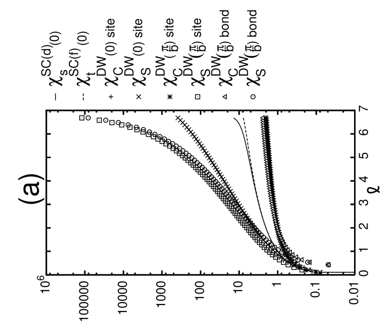
Figure 5: Flow of the susceptibilities for $2t_{\perp}/\Lambda_{0}=1.4$ (a) or $2t_{\perp}/\Lambda_{0}=1.5$ (b), and $\tilde{U}=0.5$. $\chi\lower 1.6pt\hbox{${}^{{\rm SC}(d)}_{s}(0)$}$ is the intraband singular SC susceptibility of $d$ symmetry, $\chi\lower 1.6pt\hbox{${}^{{\rm SC}(f)}_{t}$}(0)$ is the intraband triplet SC susceptibility of $f$ symmetry, $\chi^{\rm DW}_{C}(0)$ is the intraband CDW susceptibility, $\chi^{\rm DW}_{S}(0)$ is the intraband SDW susceptibility, $\chi^{\rm DW}_{C}({\pi\over b})$ is the interband CDW susceptibility and $\chi^{\rm DW}_{S}({\pi\over b})$ is the interband SDW susceptibility (the difference between site and bond susceptibilities as well as the symmetry classification are explained in part III of Ref. [22]).

In Fig. 6, the two phase diagrams are presented, according to the choice of the RG scheme. Let us repeat that, when $\Delta k_{f}$ is not renormalized, both schemes give almost the same phase diagram[35]. Here, on the contrary, one observes that the SDW region quantitatively depends on the RG scheme. Indeed, for all values of $U$, except very small ones, in the Wick-ordered calculation, a constant critical value $t_{\perp c}$ can be defined, which separates the SDW and the SC regions. In the OPI calculations, the evolution of this critical value $t_{\perp c}$ is smoother, with a linear part of slope $\sim 8.6$ at small $U$. On the whole, the critical line $t_{\perp c}(U)$ which separates both regions differs quantitatively, except for small values of $U$[37]. With the Wick-ordered RG scheme, the SDW area is reduced by a factor 3, compared to the result of the RG with the OPI scheme.

The difference of results coming from the choice of the RG scheme has already been suggested by several authors. It was, in particular mentioned in Ref. [29].

Figure 6: Phase diagram, versus parameters $t_{\perp}$ and $\tilde{U}={U\over\pi v_{\!f}}$; the central area belongs to the SDW phase, according to the OPI scheme, and to the SC one, according to the Wick-ordered scheme. The parameter $n$ indicates range $[-2n\Delta kf,2n\Delta k_{f}]$ in which $K_{\|}$ dependency is exactly taken into account. We did not distinguish the curves for $n=2$ and $n=4$ in the Wick-ordered scheme, because they hardly separate de visu.

The behaviour of the Fermi surface, during the RG flow, brings no surprise. Let us first present the results in the SC phase, then in the SDW one.

In the SC phase, $\Delta k_{f}$ increases slowly, while not diverging. The flow diverges at some $\Lambda_{c}$, and $\Delta k_{fc}$ is the final value of $\Delta k_{f}$. The numerical values of $\Delta k_{fc}/\Lambda_{0}$ are not realistic, however the general trend is very satisfactory and indicates that the binding/antibinding separation is necessary to the existence of superconductivity. We believe that, if one would include a greater number of chains in the model, one would obtain more realistic values for $\Delta k_{fc}$.

Let us emphasize the importance of a non-zero value of $\Delta k_{f}$. As discussed by Clarke, Strong and Anderson[38], the properties of Luttinger liquid, which have been established for a single one-dimensional chain, can extend in the case of a quasi-one-dimensional system (spin/charge separation, power-law behaviour of correlation functions); that is, even though the band structure extends in the $\perp$ dimension (as $\Delta k_{f}\neq 0$), the system will not converge to the two-dimensional Fermi liquid. These authors claim that $\perp$ superconductivity originates from this mechanism, which also relates to confinement in the $\|$ dimension. From this point of view, unconventional superconductivity and Luttinger liquid concept (in particular spin/charge separation) are interplaying; this gives an explanation for the possibility of coexistence of SDW instabilities and superconductivity.

In this SC phase, we also observe a quantitative difference between the results obtained using a OPI or a Wick-ordered scheme. In the first case, the value of $\Delta k_{f}$ lies in the interval $[25,30]$, while in the second, it lies in $[4,5]$ (see Fig. 7 (c) and (d)).

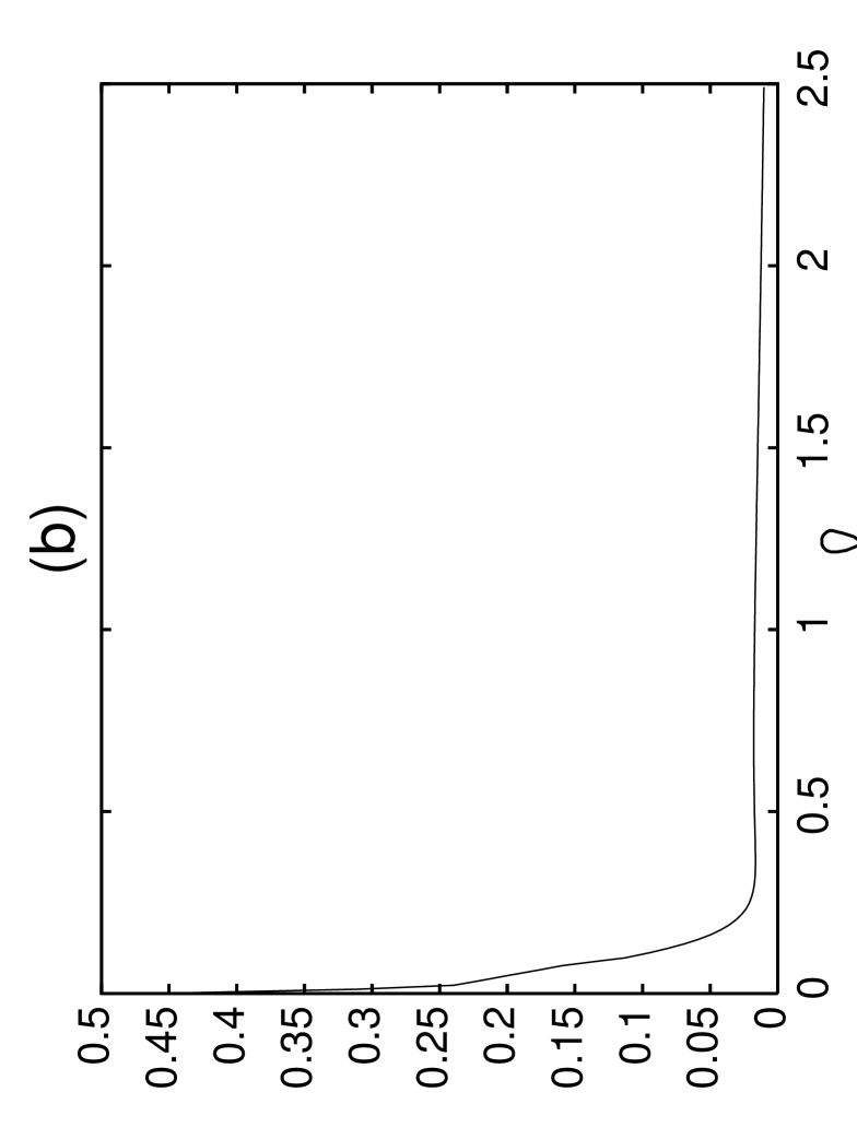
Figure 7: Flow of the $\Delta k_{f}$: in the SDW phase, (a) using OPI RG calculations, or (b) using Wick-ordered RG calculations; in the SC phase, (c) using OPI RG calculations, or (d) using Wick-ordered RG calculations.

In the SDW phase, $\Delta k_{f}\to 0$ as $\Lambda\to\Lambda_{c}$ (see Fig. 7 (a) and (b)). This proves that this phase relates to the Luttinger solution. Contrary to the SC phase, the band structure remains purely one-dimensional. This system, however, is different from Luttinger’s original one, because, in real space, there are still two chains, with non-zero hopping in-between. Let us examine in detail the behaviour of the scattering susceptibilities. Couplings $g_{01}$ and $g_{02}$ are not diverging (see Fig. 8), contrary to what is observed in the SC phase. The curves of all couplings are very close to those obtained when $\Delta k_{f}$ is kept constant. These results are very different from that of Fabrizio, who finds the behaviour of a single chain (see Ref. [21] and compare with Fig. 8 here).

Figure 8: Flow of couplings $g_{01}$ and $g_{02}$ during the RG flow, for $\tilde{U}=0.5$ and $2t_{\perp}/\Lambda_{0}=1.485$.

One must observe that, as $\Delta k_{f}\to 0$, the effective range of $K_{\|}$ shrinks, so that, when one approaches the critical scale $\Lambda_{c}$, the $K_{\|}$ dependence is extremely badly taken into account. On could even expect to recover usual RG calculations, for which no SDW phase is found; however, the observation of this phase has proved surprisingly robust; the explanation is probably that, just before $\Lambda_{c}$, the divergence of $\chi^{\rm DW}_{S}$ dominates already in such a way that it prevents any divergence of $\chi\lower 1.6pt\hbox{${}^{{\rm SC}(d)}_{s}$}$. Nevertheless, this discussion sheds also light about serious numerical convergence problems that arise in this region, and have required technical answers.

Let us compare these calculations with experimental data. No direct determination of $U$ or $t_{\perp}$ are available, one can only get indirect determinations by matching experimental and theoretical curves, as it is done in Ref. [39], for $Sr_{14-x}Ca_{x}Cu_{24}O_{41}$ compounds (with $x=12$). These authors compare several experimental and theoretical spin susceptibility curves (including uniform spin susceptibilities) and obtain a best fit for $U/t_{\|}\sim 4$ and $|t_{\perp}|\sim t_{\|}$ (those values correspond here to $\tilde{U}\sim 1$ and $2t_{\perp}\sim\Lambda_{0}$), which corresponds here to predictions done with the Wick-ordered scheme; other determinations are available, which correspond to the OPI scheme. Actually, the determinations are accurate within an order of magnitude, thus it is not possible, from experimental data, to decide which scheme gives the right predictions. However, many theoretical predictions, and a few experimental fits, are located in this region of parameters, close to point $(\tilde{U}\sim 1,2t_{\perp}/\Lambda_{0}\sim 1)$ in the phase diagram (for instance by a factor $\leavevmode\nobreak\ 2$). In particular the boundary, between SC and SDW phases, is located in the same region of parameters. Therefore, even if we can’t discriminate between Wick-ordered and OPI schemes, the phase diagrams we have calculated are qualitatively in good agreement with experimental observations.

In conclusion, we would like to emphasize that these calculations confirm the determination of a pure SDW phase using a very simple ladder model, which was far from being obvious until now. The SC phase also indicates a possible coexistence of magnetism and superconductivity, as it is indeed observed, both theoretically and experimentally.

We have also established the importance of the choice of the RG scheme. Even if this alternative only raises quantitative differences, they are not negligible, so this has to be carefully taken into account. We hope that in further and more precise models, a clear discrimination between the two schemes will be possible, and that it will confirm our conjecture that the OPI scheme is more accurate.

The authors would like to thank deeply Christoph Nickel for his collaboration in the theoretical preparation of this paper; without his help, this work would probably never have been completed successfully.

References

- [1] M. Azuma, Z. Hiroi, M. Takano, K. Ishida & Y. Kitaoka, Phys. Rev. Lett. 73, 3463 (1994).
- [2] Le Carron, Mater. Res. Bull. 23, 1355 (1988); Sigrist, ibidem, 1429.
- [3] Z. Hiroi & M. Takano, Nature 377, 41 (1995).
- [4] H. Sato & M. Naito, Physica C 274, 221 (1997).
- [5] E. Dagotto, Rep. Prog. Phys. 62, 1525 (1999).
- [6] Y. Piskunov et al, EPJ B 13, 417 (2000).
- [7] See Fig. 3 in: J. Hopkinson & K. Le Hur, Phys. Rev. B 69, 245105 (2004).
- [8] K. Kuroki, T. Kimura & H. Aoki, Phys. Rev. B 54, R15641 (1996).
- [9] J. A. Riera, Phys. Rev. B 64, 104520 (2001)
- [10] M. Randeria, N. Trivedi, A. Moreo, R. T. Scalettar, Phys. Rev. Lett. 69, 2001 (1992).
- [11] N. Bulut, D. J. Scalapino & S. R. White, Phys. Rev. B 50, 7215 (1994).
- [12] P. Germain & M. Laguës, EPJ B 8, 497 (1999).
- [13] R. M. Noack, S. R. White & D. J. Scalapino, Phys. Rev. Lett. 73, 882 (1994).
- [14] G. Sierra & M. A. Martin-Delgado, Phys. Rev. B 56, 8774 (1997).
- [15] A. Moreo, S. Haas, A. W. Sandvik & E. Dagotto, Phys. Rev. B 51, 12045 (1995).
- [16] K. G. Wilson, Phys. Rev. B 4, 3174 (1971).
- [17] K. Kuroki & H. Aoki, Phys. Rev. Lett. 72, 2947 (1994).
- [18] H. J. Schulz, Phys. Rev. B 53, R2959 (1996).
- [19] T. Giamarchi & H. J. Schulz, J. Phys. (Fr) 49, 819 (1988).
- [20] It is impossible to review the hundreds of articles using this model; three pioneer works are P. W. Anderson, Science 235, 1196 (1987), J. R. Schrieffer, X.-G. Wen & S.-C. Zhang, Phys. Rev. Lett. 60, 944 (1988) and C. L. Kane, P. A. Lee & N. Read, Phys. Rev. B 39, 6880 (1989).
- [21] M. Fabrizio, Phys. Rev. B 48, 15838 (1993).
- [22] G. Abramovici, J. C. Nickel & M. Héritier, Phys. Rev. B 72, 045120 (2005).
- [23] W. Metzner, C. Castellani & C. Di Castro, Adv. Phys. 47, 317 (1998).
- [24] C. Honerkamp, M. Salmhofer, N. Furukawa & T. M. Rice, Phys. Rev. B 63, 35109 (2001).
- [25] M. Salmhofer, Phys. Lett. B 408, 245 (1997), M. Salmhofer, Commun. Math. Phys. 194, 249 (1998).
- [26] J. Sólyom, Adv. Phys. 28, 201 (1979).
- [27] N. Dupuis, Eur. Phys. B 3, 315 (1998).
- [28] S. Dusuel & B. Douçot, Phys. Rev. B 67, 205111 (2003).
- [29] D. Rohe & W. Metzner, Phys. Rev. B 71, 115116 (2005).
- [30] A. A. Katanin & A. P. Kampf, Phys. Rev. Let. 93, 106406 (2004).
- [31] For a pedagogical explanation of the Wick-ordered scheme, see C. J. Halboth, Als Ms gedr.-Aachen: Shaker 1999, ed. Techn. Hochsch. (Aachen), Diss., 1999 (ISBN 3-8265-6822-2).
- [32] For a pedagogical explanation of the OPI scheme, see J. C. Nickel, Thèse de troisième cycle, de l’Université Paris 11 (2004).
- [33] Other choices are possible, see for instance the scheme used in: C. Bourbonnais and R. Duprat, Bulletin of the American Physical Society, 49 No. 1, 179 (2004).
- [34] In one-loop diagrams, there is only one integration, however, the domain of external momenta are different in the OPI scheme and in the Wick-ordered one.
- [35] All calculations in Ref. [22] are done using the OPI scheme. They have been also performed using the Wick-ordered scheme, but there are no noticeable differences.
- [36] D. Zanchi, Europhys. Lett. 55, 376 (2001), D. Zanchi & H. J. Schulz, Phys. Rev. B 61, 13609 (2000).
- [37] It is a fact that all curves are exactly converging to the point (), however, one has to take these extrapolations very carefully, because the theoretical precision of the calculations behaves like and one observes that for .
- [38] D. G. Clarke, S. P. Strong & P. W. Anderson, Phys. Rev. Lett. 74, 4499 (1995).
- [39] See last §(before acknowlegments) in: M. Tsuchiizu & Y. Suzumura, Phys. Rev. B 72, 075121 (2005).