Hyperfine Interactions in Graphene and Related Carbon Nanostructures

Abstract

Hyperfine interactions, magnetic interactions between the spins of electrons and nuclei, in graphene and related carbon nanostructures are studied. By using a combination of accurate first principles calculations on graphene fragments and statistical analysis, I show that both isotropic and dipolar hyperfine interactions can be accurately described in terms of the local electron spin distribution and atomic structure. A complete set of parameters describing the hyperfine interactions of ¹³C and other nuclear spins at substitution impurities and edge terminations is determined.

Graphene and related carbon nanostructures are considered as potential building blocks of future electronics, including spintronics Z̆utić et al. (2004) and quantum information processing based on electron spins Loss and DiVincenzo (1998) or nuclear spins Kane (1998). Carbon nanostructures are attractive for these applications because of the weak spin-orbit interaction in materials made of light elements Xiong et al. (2004); Bader (2006). Promising results for the spin-polarized current lifetimes in carbon nanotubes Tsukagoshi et al. (1999); Sahoo et al. (2005); Hueso et al. (2007) and graphene Hill et al. (2006) unambiguously confirm the potential of these materials. A number of quantum dot devices, components of solid-state quantum computers, based on carbon nanostructures have been proposed recently Bockrath et al. (2001); Buitelaar et al. (2002); Trauzettel et al. ; Silvestrov and Efetov (2007). Hyperfine interactions (HFIs), the weak magnetic interactions between the spins of electrons and nuclei, become increasingly important on the nanoscale. In carbon nanostructures the interactions of electron spins with an ensemble of nuclear spins are expected to be the leading contribution to the electron spin decoherence Xiong et al. (2004); Sahoo et al. (2005); Semenov et al. (2007). Minimizing HFIs is thus necessary for achieving longer electron spin coherence times Khaetskii et al. (2002). In some other instances the HFIs play an important role as a link between the spins of electrons and nuclei in the nanostructures Kane (1998); Taylor et al. (2003); Epstein et al. (2005); Childress et al. (2006) underlying the implementations of quantum information processing involving nuclear spins. Probing HFIs with magnetic resonance techniques also provides a wealth of information about structure and dynamics of carbon materials Pennington and Stenger (1996). A common understanding and an ability to control the HFIs are thus necessary for engineering future electronic devices based on graphene and related nanostructures.

In this Letter, I study the hyperfine interactions in carbon nanostructures by using a combination of accurate first principles calculations on graphene fragments and statistical analysis. I show that the interaction of the conduction (low-energy) $\pi$ electron spins with nuclear spins can be described in terms of only the local (on-site and first-nearest-neighbor) $\pi$ electron spin distribution and the local atomic structure. The conduction electron spin distribution can be determined using simpler computational approaches (e.g. tight binding or analytical approximations Nakada et al. (1996); Pereira et al. (2006)) and tuned by tailoring nanostructure dimensions and applying external fields Tifrea et al. (2003); Poggio et al. (2003). The local nature of HFIs justifies the extension of my results from small molecular models to extended systems. I further extend the considerations to curved topologies and to the presence of heteronuclei at impurities and boundaries.

The all-electron density functional theory (DFT) calculations Frisch et al were performed using a combination of the EPR-III Gaussian orbital basis set Rega et al. (1996) specially tailored for the calculations of hyperfine couplings and the B3LYP exchange-correlation hybrid density functional Becke (1988). This computational protocol (see Ref. Hermosilla et al., 2005 for details) can be applied to molecules of limited size and predicts hyperfine coupling constants (HFCCs) in excellent agreement with experimental results Hermosilla et al. (2005). Spin-orbit and relativistic effects which are not important for the calculation of HFIs in light-element systems van Lenthe et al. (1998) have been neglected. For a set of representative experimentally measured ¹³C isotropic HFCCs of graphenic ion-radicals Bolton and Fraenkel (1964) our computations provide a mean absolute error of 1.1 MHz ($\approx$2% of the range of magnitudes), which justifies the use of calculated HFCCs as a reference.

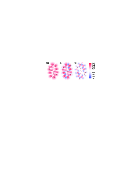
Figure 1: (Color online). Projections of the spin-polarized conduction electron density $\rho^{s}_{c}(\mathbf{r})$ (a) and the total spin density $\rho^{s}(\mathbf{r})$ (b) on the plane of an electron-doped graphene fragment (in a.u.^-2). The total spin density $\rho^{s}(\mathbf{r},z$$=$$0)$ (c) in the plane of nuclei (in a.u.^-3) reflects the isotropic hyperfine field. Molecular framework is shown by black lines.

The effective spin-Hamiltonian of the HFI between the electron spin ${\mathbf{S}}$ and the nuclear spin ${\mathbf{I}}$ can be written as $\hat{\mathbf{H}}$=${\mathbf{S}}$$\cdot$$\overleftrightarrow{\mathbf{A}}$$\cdot$${\mathbf{I}}$, where the 3$\times$3 HFI tensor $\overleftrightarrow{\mathbf{A}}$$=$$A_{iso}$$\cdot$$\overleftrightarrow{\mathbf{1}}$$+$$\overleftrightarrow{\mathbf{T}}$ is usually decomposed into the scalar HFCC $A_{iso}$ and the traceless dipolar HFI tensor $\overleftrightarrow{\mathbf{T}}$ Kaupp et al. (2004). The HFI tensor $\overleftrightarrow{\mathbf{A}}$ reflects the distribution of the electron spin density $\rho^{s}(\mathbf{r})$=$\rho^{\uparrow}(\mathbf{r})$$-$$\rho^{\downarrow}(\mathbf{r})$ viewed from the position of the nucleus $I$. In carbon nanostructures the nuclear spins are those of the ¹³C isotope ($\approx$1.1% natural abundance and can be atrificially changed; the dominant ¹²C isotope has zero spin) and other elements originating from impurities and boundaries. The electron spin density $\rho^{s}({\mathbf{r}})$ can be further decomposed into the contribution of half-populated conduction electron states lying close to the Fermi level (or singly occupied molecular orbitals in the molecular context), $\rho^{s}_{c}({\mathbf{r}})$=$\sum_{c}|\psi^{c}({\mathbf{r}})|^{2}$$\geq$0, and the contribution of the fully populated valence states perturbed by the exchange with spin-polarized conduction electrons, $\rho^{s}_{v}({\mathbf{r}})$=$\sum_{v}|\psi^{v\uparrow}({\mathbf{r}})|^{2}$$-$$|\psi^{v\downarrow}({\mathbf{r}})|^{2}$. The crucial role of the exchange-polarization effect is illustrated with a model electron-doped hydrogen-terminated graphene fragment in the doublet spin state (Fig. 1). While the projection of $\rho^{s}_{c}({\mathbf{r}})$ on the $xy$ plane (Fig. 1a) is positive everywhere and reveals an enhancement at the zig-zag edges, the projection of the total spin-density $\rho^{s}({\mathbf{r}})$ (Fig. 1b) is negative where $\rho^{s}_{c}({\mathbf{r}})$ is close to zero. The isotropic (Fermi contact) HFCC is proportional to the total spin density at the position of nucleus $I$, $A_{iso}$$=$$(4\pi/3S)\beta_{e}\beta_{N}g_{e}g_{I}\rho^{s}({\mathbf{r}}_{I})$, where $\beta_{e}$ and $\beta_{N}$ are the Bohr and nuclear magnetons, while $g_{e}$ and $g_{I}$ are the $g$-values of free electron and nucleus $I$, respectively. $S$ is the maximum value of the electron spin projection. For the ideal graphene and planar $sp^{2}$ carbon nanostructures (all nuclei lie in the $z$=0 plane) $\rho^{s}_{c}(z$=$0)$=0 due to the $p_{z}$ symmetry of the conduction states. However, there is a contribution of the $\sigma$ symmetry valence states $\rho^{s}_{v}(z$=$0)$$\neq$0 due to the exchange-polarization effect. For the model graphene fragment $\rho^{s}_{v}(z$=$0)$ (Fig. 1c) shows an alternating pattern with a relative dominance of the negative spin density. Since the $\sigma$ states are situated well above and well below the Fermi level in $sp^{2}$ carbon nanostructures, the valence exchange-polarization phenomenon exhibits the property of locality. This property was exploited by Karplus and Fraenkel almost 50 years ago to describe the isotropic ¹³C HFCCs in conjugated organic radicals Karplus and Fraenkel (1961). The main contribution to the hyperfine anisotropy originates from the total spin population $n$ of the on-site $p_{z}$ atomic orbital, which also incorporates the contribution of exchange-polarized valence states. Assuming a local axial symmetry, $\overleftrightarrow{\mathbf{T}}$ can be written as a diagonal matrix with elements $T_{zz}$/2=$-T_{xx}$=$-T_{yy}$=$A_{dip}$, where $A_{dip}$=$(1/5S)\beta_{e}\beta_{N}g_{e}g_{I}n\langle 1/r_{2p}^{3}\rangle$ ($r_{2p}$ is the distance of the carbon $2p$ electron to nucleus).

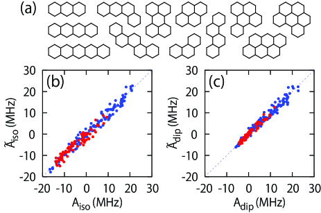
Figure 2: (Color online) (a) Set of graphene fragments used in the present calculations. Fitted Fermi contact ($\tilde{A}_{iso}$) and dipolar ($\tilde{A}_{dip}$) ¹³C HFCCs vs the corresponding values, $A_{iso}$ (b) and $A_{dip}$ (c), calculated from first principles. The values for inner (3 carbon NNs) and boundary (2 carbon NNs) atoms are shown as red and blue dots, respectively.

Table 1: Parameters (in MHz) fitted to the results of calculations of a set of nanographite molecules.

	$a_{2}$	$a_{3}$	$b_{2}$	$b_{3}$	$c$	$d$
$A_{iso}$	162	128	2.3	6.1	-57.4	-7.4
$A_{dip}$	155	131	2.7	3.6	-19.4	-12.8

The HFIs were calculated for a set of 12 ($\sim$1 nm size) electron- and hole-doped planar hydrogen terminated graphene fragments (Fig. 2a) in the spin-doublet ground states. This provides overall statistics for 206 inequivalent ¹³C HFCCs. The calculated $A_{iso}$ and $A_{dip}$ values are fitted to the extended form of the Karplus-Fraenkel expression

$$A=a_{j}(1+\sum_{i\in NN}b_{j}\Delta r_{i})n^{c}+c\sum_{i\in NN}(1+d\Delta r_{i})n^{c}_{i},$$ (1)

where the two terms account for the contributions of the on-site and nearest neighbor (NN) conduction electron spin populations per unpaired electron, $n^{c}$ and $n^{c}_{i}$, respectively, calculated from first principles. The on-site coefficients $a_{j}$ and $b_{j}$ are distinguished for the cases of C atoms with 3 carbon NNs ($j$=3) and the boundary atoms with 2 carbon NNs ($j$=2). The C–C bond length effects are encountered through the coefficients $b_{j}$ and $d$ with $\Delta r_{i}$$=$$r_{i}$$-$$r_{0}$ being the deviation of the bond length $r_{i}$ from the value for the ideal graphene, $r_{0}$=1.42 Å. Only statistically significant local properties were included in the linear expression (1). The results of the regressions are summarized in Tab. 1 (1 MHz=4.136$\times$10^-3 $\mu$eV). Fig. 2(b,c) shows the fitted (using expr. (1) and regression parameters) values $\tilde{A}_{iso}$ ($\tilde{A}_{dip}$) versus the calculated $A_{iso}$ ($A_{dip}$) values. Regressions to the linear expression (1) provide accurate estimations (root-mean-square-errors are 1.7 MHz and 1.2 MHz for $A_{iso}$ and $A_{dip}$, respectively). The calculated isotropic HFCCs span about the same range of magnitudes ($-$16.7 MHz$<$$A_{iso}$$<$21.1 MHz) as the dipolar HFCCs ($-$5.9 MHz$<$$A_{dip}$$<$22.7 MHz). The HFCCs of boundary atoms tend to be larger due to the fact that low-energy states localize at the zigzag graphene edges Nakada et al. (1996). The on-site and the NN exchange-polarization effects have competitive character ($a_{3}$/$c$$\approx$$-$2) in the case of isotropic HFCCs. Our calculations predict $\approx$50% larger values for the parameters $a_{2}$, $a_{3}$ and $c$ for $A_{iso}$ compared to those obtained by Karplus and Fraenkel in their early studies of HFCCs in molecular radicals ($a_{2}$=$99.8$ MHz, $a_{3}$=$85.5$ MHz and $c$=$-$39 MHz) Karplus and Fraenkel (1961). This difference can be explained by the incorporation (via DFT) of the electron correlation effects in our calculations and to the local atomic structure of the graphene lattice. Both $A_{iso}$ and $A_{dip}$ show a tendency to enhance the on-site and to weaken the NN contributions with the increase of C–C bond lengths. The dipolar HFCC is mostly influenced by the on-site contribution of the half-populated conduction state and the NN exchange-polarization effect is weaker in this case ($a_{3}$/$c$$\approx$$-$7). When compared to typical solid state environments based on heavier elements, the ¹³C HFCCs in graphene and related nanostructures are weaker (e.g. 117 MHz ³¹P Fermi contact HFCC for the P shallow donor in Si Overhof and Gerstmann (2004)) and more anisotropic.

The graphene honeycomb lattice is a bipartite lattice, i.e. it can be partitioned into two complementary sublattices $A$ and $B$. I discuss the HFIs for the three general cases of conduction electron spin distributions over the sublattices: (i) ferromagnetic $n^{c}_{A}$=$n^{c}_{B}$$>$$0$; (ii) ferrimagnetic $n^{c}_{A}$$>$$0$ and $n^{c}_{B}$=0 and (iii) antiferromagnetic $n^{c}_{A}$=$-n^{c}_{B}$$>$$0$ (see Tab. 2). The first case can be physically realized upon the uniform magnetization of the system with equivalent $A$ and $B$ sublattices, e.g. by applying an external magnetic field. The negative $A_{iso}$$=$$-$44 MHz is small due to the partial compensation of the on-site and the NN exchange-polarization effects. This value is consistent with the values derived from the experimental ¹³C Knight shifts in graphite intercalates ($-$25 MHz$<$$A_{iso}$$<$$-$50 MHz) Conard et al. (1980) and with the calculated isotropic Knight shifts in metallic carbon nanotubes Yazyev and Helm (2005). The ferrimagnetic case with the conduction state distributed over the atoms of only one sublattice ($A$) is physically realized at the zigzag edges Nakada et al. (1996) and around single-atom point defects in sublattice $B$ Kelly and Halas (1998). Considerable alternating Fermi contact and dipolar HFCCs are predicted in this case. An antiferromagnetic pattern can be realized in the case of heavily disordered systems with localized defect and edge states in both sublattices Yazyev and Helm (2007). The magnitudes of HFIs are minimized and maximized in the cases of ferromagnetic and antiferromagnetic electron spin distributions, respectively.

Table 2: Hyperfine coupling constants for three general cases of spin populations $n^{c}$ of the carbon atoms of $A$ and $B$ sublattices of graphene.

	$A_{iso}$(A)/$n^{c}$	$A_{iso}$(B)/$n^{c}$	$A_{dip}$(A)/$n^{c}$	$A_{dip}$(B)/$n^{c}$
$n^{c}_{A}$=$n^{c}_{B}$$>$$0$	-44	-44	73	73
$n^{c}_{A}$$>$$0$; $n^{c}_{B}$=0	128	-172	131	-58
$n^{c}_{A}$=$-n^{c}_{B}$$>$$0$	300	-300	189	-189

Many carbon nanostructures of reduced dimensionality (e.g. nanotubes and fullerenes) represent non-planar topologies. Local curvatures lead to the $sp^{2}$$-$$sp^{3}$ rehybridization of carbon atoms and enable a Fermi contact interaction involving the low-energy $\pi$ electron spins Pennington and Stenger (1996). This results in a positive contribution of the $\pi$ states unless $n^{c}$ is close to zero: a contribution due to the NN exchange-polarization effect is negative in this case. The degree of rehybridization $m$ of the $\pi$ states ($s^{m}p$) can be described using a local bond angles analysis Haddon (1986). For the case of large curvature radii the original expression for $m$ can be reformulated in a more convenient form, $m$=$d_{cc}^{2}/8(1/R_{1}+1/R_{2})^{2}$, where $d_{cc}$ is the C–C distance, $R_{1}$ and $R_{2}$ are the principal curvature radii. The curvature-induced contribution to the Fermi contact ¹³C HFCC is then $A_{iso}^{curv}$$=$$(4\pi/3S)\beta_{e}\beta_{N}g_{e}g_{I}nm\phi_{2s}^{2}(0)$, where $\phi_{2s}(0)$ is the magnitude of the carbon atomic $2s$ wavefunction at the point of nucleus ($(8\pi/3)\beta_{e}\beta_{N}g_{e}g_{I}\phi_{2s}^{2}(0)$$\approx$3.5$\times$10³ MHz). The curvature-induced direct coupling becomes significant ($m$$>$$10^{-2}$) only in ultranarrow carbon nanotubes ($d$$<$1 nm) and fullerenes.

Table 3: Parameters (in MHz) describing the HFIs of nuclei of susbtitutional impurities (¹¹B and ¹⁴N), monoatomic functional groups (¹H and ¹⁹F) and rehybridized ($sp^{3}$) carbon atoms (¹³C) at the edges.

		$A_{iso}$		$A_{dip}$
Nucleus	Position	a	c	a	c
11B	subst. impurity	43	-31	60	6
14N	subst. impurity	150	-22	130	-10
1H	C${}_{sp^{2}}$ edge	-119	22
19F	C${}_{sp^{2}}$ edge	240	-40
1H	C${}_{sp^{3}}$ edge		350
19F	C${}_{sp^{3}}$ edge		750
13C	C${}_{sp^{3}}$ edge		-68

Since the natural abundance of the “HFI-active” ¹³C isotope is small ($\approx$1%), consideration of the nuclei of other elements is important for a complete description of HFIs in carbon nanostructures. The common substitution impurities are boron and nitrogen with all natural isotopes having nuclear spins. Graphene edges can be terminated by hydrogen and fluorine atoms with both ¹H and ¹⁹F spin-1/2 nuclei (99.9885% and 100% natural abundance, respectively) having high $g$-values ($g(^{1}$H$)/g(^{13}$C$)$$\approx$$g(^{19}$F$)/g(^{13}$C$)$$\approx$4). I consider HFIs in a reduced set of molecular fragments (only 3- and 4-ring structures included) with impurities and edge functionalizations in all possible positions. The calculated HFCCs have been fitted to the Karplus-Fraenkel relation, with no $\Delta r$ terms included (Tab. 3). The variations of the local charge density of states in the vicinity of impurities does not have any significant influence on HFIs. Both Fermi contact and dipolar HFCCs of the impurity nuclear spins show a monotonic increase along the ¹¹B–¹³C–¹⁴N series when compared to the results for ¹³C HFCCs (Tab. 1). The NN relative exchange-polarization effects ($a/c$ ratio) on the Fermi contacts HFCCs tend to decrease along the series. While the HFIs of the nuclear spins in substitution impurities are highly anisotropic, the hyperfine couplings of the edge nuclei show small anisotropy due to the $sp^{3}$ character of bonding. When ¹H and ¹⁹F edge nuclei are bound to the C${}_{sp^{2}}$ atoms, the isotropic HFCCs are of the same order of magnitude as those of the ¹³C spins in the graphene lattice. The influence of the NN carbon atoms (second NNs to the terminating atom) is very similar for ¹H and ¹⁹F nuclei and smaller than in the case of ¹³C HFCCs ($a_{H}/c_{H}$$\approx$$a_{F}/c_{F}$$\approx$$-$6). The spin polarization effect on ¹⁹F HFCCs is stronger and of opposite sign compared to that of protons ($a_{F}/a_{H}$$\approx$$c_{F}/c_{H}$$\approx$$-$2). When edge atoms are bound to the rehybridized ($sp^{3}$) carbon atoms, $n^{c}$ is zero but the NN contribution is significantly enhanced. The NN contribution to the ¹³C hyperfine coupling of the $sp^{3}$ edge carbon atom itself ($c$=$-$68 MHz) has a similar magnitude as that of the $sp^{2}$ edge atoms ($c$=$-$57 MHz). HFIs with the boundary spins (H-terminated edges are often obtained in experiments Kobayashi et al. (2006)) have to be taken into account when designing carbon-based nanoscale devices for spintronics or quantum computing. A chemical modification of the graphene edges (e.g. substitution of the hydrogen atoms by alkyl-groups) can be suggested to reduce electron spin decoherence effects from the HFIs with boundary spins.

In conclusion, the results of first principles calculations show that the hyperfine interactions in graphene and related nanostructures are defined by the local distribution of the conduction electron spins and by the local atomic structure. A complete set of parameters describing the hyperfine interactions was determined for the ¹³C and other common nuclear spins. These results will permit control of the magnetic interactions between the spins of electrons and nuclei by tailoring the chemical and isotopic compositions, local atomic structures, and strain fields in $sp^{2}$ carbon nanostructures. Some practical recipes for minimizing interactions with nuclear spins are given.

I acknowledge D. Loss and Yu. G. Semenov for motivating discussions, and S. Arey, D. Bulaev, L. Helm, V. G. Malkin, D. Stepanenko, and I. Tavernelli for comments on the manuscript. I also thank the Swiss NSF for financial support and CSCS Manno for computer time.

References

- Z̆utić et al. (2004) I. Z̆utić, J. Fabian, and S. Das Sarma, Rev. Mod. Phys. 76, 323 (2004).
- Loss and DiVincenzo (1998) D. Loss and D. P. DiVincenzo, Phys. Rev. A 57, 120 (1998).
- Kane (1998) B. E. Kane, Nature 393, 133 (1998).
- Xiong et al. (2004) Z. H. Xiong, D. Wu, Z. V. Vardeny, and J. Shi, Nature 427, 821 (2004).
- Bader (2006) S. D. Bader, Rev. Mod. Phys. 78, 1 (2006).
- Tsukagoshi et al. (1999) K. Tsukagoshi, B. W. Alphenaar, and H. Ago, Nature 401, 572 (1999).
- Sahoo et al. (2005) S. Sahoo, T. Kontos, C. Schönenberger, and C. Sürgers, Appl. Phys. Lett. 86, 112109 (2005).
- Hueso et al. (2007) L. E. Hueso, J. M. Pruneda, V. Ferrari, G. Burnell, J. P. Valdés-Herrera, B. D. Simons, P. B. Littlewood, E. Artacho, A. Fert, and N. D. Mathur, Nature 445, 410 (2007).
- Hill et al. (2006) E. W. Hill, A. K. Geim, K. Novoselov, F. Schedin, and P. Blake, IEEE Trans. Magn. 42, 2694 (2006).
- Bockrath et al. (2001) M. Bockrath, W. Liang, D. Bozovic, J. H. Hafner, C. M. Lieber, M. Tinkham, and H. Park, Science 291, 283 (2001).
- Buitelaar et al. (2002) M. R. Buitelaar, A. Bachtold, T. Nussbaumer, M. Iqbal, and C. Schönenberger, Phys. Rev. Lett. 88, 156801 (2002).
- (12) B. Trauzettel, D. V. Bulaev, D. Loss, and G. Burkard, Nat. Phys. 3, 192 (2007).
- Silvestrov and Efetov (2007) P. G. Silvestrov and K. B. Efetov, Phys. Rev. Lett. 98, 016802 (2007).
- Semenov et al. (2007) Y. G. Semenov, K. W. Kim, and G. J. Iafrate, Phys. Rev. B 75, 045429 (2007).
- Khaetskii et al. (2002) A. V. Khaetskii, D. Loss, and L. Glazman, Phys. Rev. Lett. 88, 186802 (2002).
- Taylor et al. (2003) J. M. Taylor, C. M. Marcus, and M. D. Lukin, Phys. Rev. Lett. 90, 206803 (2003).
- Epstein et al. (2005) R. J. Epstein, F. M. Mendoza, Y. K. Kato, and D. D. Awschalom, Nat. Phys. 1, 94 (2005).
- Childress et al. (2006) L. Childress, M. V. G. Dutt, J. M. Taylor, A. S. Zibrov, F. Jelezko, J. Wrachtrup, P. R. Hemmer, and M. D. Lukin, Science 314, 281 (2006).
- Pennington and Stenger (1996) C. H. Pennington and V. A. Stenger, Rev. Mod. Phys. 68, 855 (1996).
- Nakada et al. (1996) K. Nakada, M. Fujita, G. Dresselhaus, and M. S. Dresselhaus, Phys. Rev. B 54, 17954 (1996).
- Pereira et al. (2006) V. M. Pereira, F. Guinea, J. M. B. Lopes dos Santos, N. M. R. Peres, and A. H. Castro Neto, Phys. Rev. Lett. 96, 036801 (2006).
- Tifrea et al. (2003) I. Ţifrea and M. E. Flatté, Phys. Rev. Lett. 90, 237601 (2003).
- Poggio et al. (2003) M. Poggio, G. M. Steeves, R. C. Myers, Y. Kato, A. C. Gossard, and D. D. Awschalom, Phys. Rev. Lett. 91, 207602 (2003).
- (24) The Gaussian03 code [M. J. Frisch et al., Gaussian03, Rev. C.02, Gaussian, Inc., Wallingford, CT, 2004] was used.
- Rega et al. (1996) N. Rega, M. Cossi, and V. Barone, J. Chem. Phys. 105, 11060 (1996).
- Becke (1988) A. D. Becke, Phys. Rev. A 38, 3098 (1988); C. Lee, W. Yang, and R. G. Parr, Phys. Rev. B 37, 785 (1988); A. D. Becke, J. Chem. Phys. 98, 5648 (1993).
- Hermosilla et al. (2005) L. Hermosilla, P. Calle, J. M. García de la Vega, and C. Sieiro, J. Phys. Chem. A 109, 1114 (2005).
- van Lenthe et al. (1998) E. van Lenthe, A. van der Avoird, and P. E. S. Wormer, J. Chem. Phys. 108, 4783 (1998).
- Bolton and Fraenkel (1964) J. R. Bolton and G. K. Fraenkel, J. Chem. Phys. 40, 3307 (1964); D. J. M. Fassaert and E. de Boer, Recl. Trav. Chim. Pays-Bas 91, 273 (1972); R. F. Claridge, C. M. Kirk, and B. M. Peake, Aust. J. Chem. 26, 2055 (1973).
- Kaupp et al. (2004) M. Kaupp, M. Bühl, and V. G. Malkin, eds., Calculation of NMR and EPR parameters: Theory and Applications (Wiley-VCH: Weinheim, 2004).
- Karplus and Fraenkel (1961) M. Karplus and G. K. Fraenkel, J. Chem. Phys. 35, 1312 (1961).
- Overhof and Gerstmann (2004) H. Overhof and U. Gerstmann, Phys. Rev. Lett. 92, 087602 (2004).
- Conard et al. (1980) J. Conard, H. Estrade, P. Lauginie, H. Fuzellier, G. Furdin, and R. Vasse, Physica B 99, 521 (1980).
- Yazyev and Helm (2005) O. V. Yazyev and L. Helm, Phys. Rev. B 72, 245416 (2005).
- Kelly and Halas (1998) K. Kelly and N. Halas, Surf. Sci. 416, L1085 (1998).
- Yazyev and Helm (2007) O. V. Yazyev and L. Helm, Phys. Rev. B 75, 125408 (2007).
- Haddon (1986) R. C. Haddon, J. Am. Chem. Soc. 108, 2837 (1986).
- Kobayashi et al. (2006) Y. Kobayashi, K. I. Fukui, T. Enoki, and K. Kusakabe, Phys. Rev. B 73, 125415 (2006).