Symmetry constraints on phonon dispersion in graphene

Abstract

Taking into account the constraints imposed by the lattice symmetry, the phonon dispersion is calculated for graphene with interactions between the first and second nearest neighbors in the framework of the Born-von Karman model. Analytical expressions are obtained for the out-of-plane (bending) modes determined only by two force constants as well as for the in-plane modes with four force constants. Values of the force constants are found in fitting to elastic constants and Raman frequencies observed in graphite.

I Introduction

Since the discovery of graphene (a single atomic layer of graphite) Novo ; ZSA , main attention has been devoted to its electronic properties. More recently, Raman spectroscopy FMS extends to investigations of graphene. For interpretations of the Raman scattering as well as of the transport phenomena, the detailed knowledge of the lattice dynamics and the electron-phonon interactions is needed NG .

Several models DL ; NWS ; AR ; NB ; MKH ; AD ; GMR ; LDC have been proposed to calculate the phonon dispersion in bulk graphite. Most improved ones MKH ; AD involve many (up to twenty) parameters. Recently, detailed measurements and first-principles calculations of optical phonon frequencies were made for graphite MRTR ; MMD . They show the qualitative disagreement with the models DL ; LDC , which include the central and angular atomic forces between the first and second neighbors in the graphite lattice.

The passage in the lattice dynamics from graphite to graphene and then to nanotubes was examined in the ab initio calculation SAS ; DK , in Ref. CMC using the model DL , and in Ref. GSK up to the fourth neighbor with 12 force constants. Numerical calculations based on Hückel’s theory MCZ and in terms of the electron energy were performed in work PL . The first-principles calculations MM of dynamical properties for graphite and graphene (and also for diamond) show that distinctions between the phonon frequencies in graphene and relating ones in graphite are negligible in comparison with the experimental errors for that frequencies in graphite. For the highest frequencies, this could be intuitively expected because interactions between the adjacent layers in graphite are weak.

Our aim here is to find an analytical description of the phonon dispersion in graphene. This can be done within the framework of the Born-von-Karman model for the honeycomb graphene lattice with interactions only between first and second nearest neighbors, but the constraints imposed by the lattice symmetry should be taken into account. We show that the out-of-plane (bending) and in-plane modes are decoupled from each other. The out-of-plane modes are described by two force constants determined in fitting to the Raman frequency and smallest elastic constant $C_{44}$. In the narrow wave-vector interval near the $\Gamma$ point, the acoustic out-of-plane mode has a linear dispersion with the non-zero sound velocity in contrast to the so-called membrane mode which demonstrates the quadratic dispersion in the continuous-medium approximation LL . We do not pay close attention to the agreement of lower frequencies with experiments on graphite because their values in graphene are convincingly less that ones in graphite. The four force constant describing the in-plane modes are found in fitting to their Raman frequencies and elastic constant $C_{11}$ and $C_{12}$ of graphite. The extent of agreement of the present theory with experiments corresponds to the comparison level between the first-principal calculations MRTR and their data (see Table 3).

II Phonon dynamics in nearest neighbor approximation

The equations of moution in the harmonic approximation are written in the well-known form

$$\sum\limits_{j,m,\kappa^{\prime}}\Phi^{\kappa\kappa^{\prime}}_{ij}({\bf a}_{n}-{\bf a}_{m})u_{j}^{\kappa^{\prime}}({\bf a}_{m})-\omega^{2}u_{i}^{\kappa}({\bf a}_{n})=0,$$ (1)

where the vectors ${\bf a}_{n}$ numerate the lattice cells, the superscripts $\kappa,\kappa^{\prime}$ note two sublattices $A$ and $B$, and the subscripts $i,j=x,y,z$ take three values corresponding to the space coordinates. Since the potential energy is the quadratic function of the atomic displacements $u^{A}_{i}({\bf a}_{n})$ and $u^{B}_{i}({\bf a}_{n})$, the force-constant matrix can be taken in the symmetric form, $\Phi_{ij}^{AB}({\bf a}_{n})=\Phi_{ji}^{BA}(-{\bf a}_{n}),$ and its Fourier transform, i.e. the dynamical matrix, is a Hermitian matrix.

Each atom, for instance, ${\bf A}_{0}$ (see Fig. 1) has three first neighbors in the other sublattice, i. e., $B$ with the relative vectors

$${\bf B}_{1}=a(1,0),\quad{\bf B}_{2,3}=a(-1,\pm\sqrt{3})/2,$$

and six second neighbors in the same sublattice $A$ with the relative vectors

$${\bf A}_{1,4}= \pm a(0,\sqrt{3}),\quad{\bf A}_{2,5}=\pm a(-3,\sqrt{3})/2,$$

$${\bf A}_{3,6}=\mp a(3,\sqrt{3})/2,$$

where $a=1.42\AA$ is the carbon-carbon distance.

For the nearest neighbors (in the $B$ sublattice), the dynamical matrix has the form

$$\phi^{AB}_{ij}({\bf q})=\sum_{\kappa=1}^{3}\Phi^{AB}_{ij}({\bf B}_{\kappa})\exp(i{\bf qB}_{\kappa}),$$ (2)

and for the next neighbors (in the $A$ sublattice)

$$\phi^{AA}_{ij}({\bf q})=\Phi^{AA}_{ij}({\bf A}_{0})+\sum_{\kappa=1}^{6}\Phi^{AA}_{ij}({\bf A}_{\kappa})\exp(i{\bf qA}_{\kappa}),$$ (3)

where ${\bf A}_{0}$ indices the atom chosen at the center of the coordinate system in the $A$ sublattice and the wave vector ${\bf q}$ is taken in units of $1/a$.

Figure 1: First and second neighbors in the graphene lattice.

The point group $D_{6h}$ of the honeycomb lattice is generated by $\{C_{6},\sigma_{v},\sigma_{z}\}$, where $\sigma_{z}$ is a reflection $z\to-z$ by the plane that contains the graphene layer, $C_{6}$ is a rotation by $\pi/3$ around the $z$ axis, and $\sigma_{v}$ is a reflection by the $xz$ plane. The transformations of the group impose constraints on the dynamical matrix. To obtain them, we introduce variables $\xi,\eta=x\pm iy$ transforming under the rotation $C_{3}$ around the $z$-axis (taken at the ${\bf A}_{0}$ atom) as follows $(\xi,\eta)\rightarrow(\xi,\eta)\exp(\pm 2\pi i/3)$. In the rotation, the atoms change their positions ${\bf B}_{1}\rightarrow{\bf B}_{2}\rightarrow{\bf B}_{3}$, ${\bf A}_{1}\rightarrow{\bf A}_{3}\rightarrow{\bf A}_{5}$, and ${\bf A}_{2}\rightarrow{\bf A}_{4}\rightarrow{\bf A}_{6}$. Therefore, all the force constants $\Phi^{AB}_{\xi\eta}({\bf B}_{\kappa})$ with the different $\kappa$ (as well as $\Phi^{AB}_{zz}({\bf B}_{\kappa})$) are equal to one another, but the force constants with the coincident subscripts $\xi$ or $\eta$ transform as covariant variables. For instance,

$$\Phi^{AB}_{\xi\xi}({\bf B}_{1})=\Phi^{AB}_{\xi\xi}({\bf B}_{2})\exp{(2\pi i/3)}$$ (4)

$$=\Phi^{AB}_{\xi\xi}({\bf B}_{3})\exp{(-2\pi i/3)}.$$

The relation between $\Phi^{AA}_{\xi\xi}({\bf A}_{\kappa})$ with the points ${\bf A}_{1},{\bf A}_{3},{\bf A}_{5}$ (and also between ${\bf A}_{4},{\bf A}_{2},{\bf A}_{6}$) has the same form. The constants $\alpha_{z}=\Phi^{AB}_{zz}({\bf B}_{1}),\gamma_{z}=\Phi^{AA}_{zz}({\bf A}_{1}),\alpha=\Phi^{AB}_{\xi\eta}({\bf B}_{1}),$ and $\gamma=\Phi^{AA}_{\xi\eta}({\bf A}_{1})$ are evidently real. The constant $\beta=\Phi^{AB}_{\xi\xi}({\bf B}_{1})$ is real because the reflection $(x,y)\rightarrow(x,-y)$ with ${\bf B}_{1}\rightarrow{\bf B}_{1}$ belongs to the symmetry group. Besides, for the first and second neighbors, we have one complex force constant $\delta=\Phi^{AA}_{\xi\xi}({\bf A}_{1})$.

Two force constants $\Phi^{AA}_{zz}({\bf A}_{0})$ and $\Phi^{AA}_{\xi\eta}({\bf A}_{0})$ for the atom ${\bf A}_{0}$ can be excluded with the help of conditions imposed by invariance with respect to the translations of the layer as a whole in the $x/z$ directions. Using the equations of motion (1) and Eqs. (2), (3), we find this stability condition

$$\Phi^{AA}_{\xi\eta}({\bf A}_{0})+6\Phi^{AA}_{\xi\eta}({\bf A}_{1})+3\Phi^{AB}_{\xi\eta}({\bf B}_{1})=0$$ (5)

and the similar form for the $zz$ components.

II.1 Dispersion of the bending out-of plane modes.

In the first- and second-neighbor approximation, the out-of-plane vibrations $u_{z}^{A},u_{z}^{B}$ in the $z$ direction are not coupled with the in-plane modes because the force constants of type $\Phi_{xz}$ or $\Phi_{yz}$ equals zero due to the reflection $z\to-z$. The corresponding dynamical matrix for the out-of-plane modes has the form

$$\left(\begin{array}[]{cc}\phi^{AA}_{zz}({\bf q})&\phi^{AB}_{zz}({\bf q})\\ \phi^{AB}_{zz}({\bf q})^{*}&\phi^{AA}_{zz}({\bf q})\end{array}\right),$$ (6)

where

$$\phi^{AA}_{zz}({\bf q})=$$

$$2\gamma_{z}[\cos{(\sqrt{3}q_{y})}+2\cos{(3q_{x}/2)}\cos{(\sqrt{3}q_{y}/2)}-3]-3\alpha_{z},$$

$$\phi^{AB}_{zz}({\bf q})=$$ (7)

$$\alpha_{z}[\exp{(iq_{x})}+2\exp{(-iq_{x}/2)}\cos{(\sqrt{3}q_{y}/2)}].$$

The phonon dispersion for the out-of-plane modes is found

$$\omega_{\text{ZO,ZA}}({\bf q})=\sqrt{\phi^{AA}_{zz}({\bf q})\pm|\phi^{AB}_{zz}({\bf q})|}.$$ (8)

The equations allow us to express the phonon frequencies of the out-of plane branches at the critical points $\Gamma,K$, and $M$ in terms of the force constants:

$$\omega_{\text{ZO}}(\Gamma)=\sqrt{-6\alpha_{z}},\quad\omega_{\text{ZO, ZA}}(K)=\sqrt{-3\alpha_{z}-9\gamma_{z}},$$ (9)

$$\omega_{\text{ZO, ZA}}(M)=\sqrt{(-3\mp 1)\alpha_{z}-8\gamma_{z}}.$$

Expanding Eq. (8) in powers of the wave vector $\bf{q}$, we find the velocity of the acoustic out-of-plane mode propagating in the layer

$$s_{z}=a\left[-0.75\alpha_{z}-4.5\gamma_{z}\right]^{1/2}=\sqrt{C_{44}/\rho},$$ (10)

where we use the well-known formula for the velocity of the acoustic $z$-mode propagating in the $x$-direction in terms of the elastic constant $C_{44}$ and density $\rho$ of a hexagonal crystal. Because the interaction between the layers in graphite is weak, we can correspond the values of $C_{44}$ and $\rho$ to graphite. Using the values of $\alpha_{z}$ and $\gamma_{z}$ obtained in fitting to the exprimental data (see Table 1), we find the value of the sound velocity for the out-plane mode $s_{z}=1.57\times 10^{5}$ cm/s.

II.2 Dispersion of the in-plane modes.

The dynamical matrix for the in-plane vibrations has the form similar to that for the in-plane mode (6), but instead of the functions $\phi_{zz}^{AA}({\bf q})$ and $\phi_{zz}^{AB}({\bf q})$ we have to substitute respectively the $2\times 2$ matrices

$$\phi^{AA}({\bf q})=\left(\begin{array}[]{cc}\phi^{AA}_{\xi\eta}({\bf q})&\phi^{AA}_{\xi\xi}({\bf q})\\ \phi^{AA}_{\xi\xi}({\bf q})^{*}&\phi^{AA}_{\xi\eta}({\bf q})\end{array}\right),$$ (11)

$$\phi^{AB}({\bf q})=\left(\begin{array}[]{cc}\phi^{AB}_{\xi\eta}({\bf q})&\phi^{AB}_{\xi\xi}({\bf q})\\ \phi^{AB}_{\eta\eta}({\bf q})&\phi^{AB}_{\xi\eta}({\bf q})\end{array}\right).$$ (12)

The matrix elements $\phi^{AA}_{\xi\eta}({\bf q})$ and $\phi^{AB}_{\xi\eta}({\bf q})$ are obtained from $\phi^{AA}_{zz}({\bf q})$ and $\phi^{AB}_{zz}({\bf q})$, Eqs. (7), respectively, with substitutions $\gamma$ and $\alpha$ instead of $\gamma_{z}$ and $\alpha_{z}$. The off-diagonal elements are given by

$$\phi^{AA}_{\xi\xi}({\bf q})=$$ (13)

$$\delta[\exp(i\sqrt{3}q_{y})+2\cos{(3q_{x}/2+2\pi/3)}\exp(-i\sqrt{3}q_{y}/2)]+$$

$$\delta^{*}[\exp(-i\sqrt{3}q_{y})+2\cos{(3q_{x}/2-2\pi/3)}\exp{(i\sqrt{3}q_{y}/2)}],$$

$$\phi^{AB}_{\xi\xi}({\bf q})=$$

$$\beta[\exp{(iq_{x})}+2\exp{(-iq_{x}/2)}\cos{(\sqrt{3}q_{y}/2-2\pi/3)}].$$

The matrix elements for the $B$ sublattice can be obtained from that ones for the $A$ sublattice by $C_{2}$ rotation $(x,y)\rightarrow-(x,y)$ of the graphene symmetry group.

The optical phonon frequencies for the in-plane branches at $\Gamma$ and $K$ are found

$$\omega_{1,2}^{in-pl}(\Gamma)=\sqrt{-6\alpha},\quad\text{doublet},$$

$$\omega^{in-pl}_{1,2}(K)=\sqrt{-3\alpha-9\gamma},\quad\text{doublet},$$ (14)

$$\omega^{in-pl}_{3,4}(K)=\sqrt{-3\alpha-9\gamma\pm 3\beta}.$$

Using Eqs. (11)-(13), we find the in-plane mode dispersion in the explicit form for the $G-K$ direction. An algebraic equation of the forth order have to be solved for the M point as well as for points of the general position.

The in-plane vibrations make a contribution into the elastic constants C₁₁ and C₁₂. The corresponding relation between the dynamic matrix elements and the elastic constants can be deduced taking the long-wavelength limit (${\bf q}\rightarrow 0$) in the matrices (11) and (12). In this limit, separating the acoustic vibrations ${\bf u}^{\text{ac}}$ from the optical modes, we obtain the equation of motion in the matrix form

$$\begin{array}[]{c}\left[(\phi^{AA}+\phi^{AB}+\phi^{BB}+\phi^{BA})/2\right.\\ +\left.\phi_{1}^{AB}(\phi_{0}^{AB})^{-1}\phi_{1}^{AB}-\omega^{2}\right]{\bf u}^{\text{ac}}=0,\end{array}$$ (15)

where the subscripts 0 and 1 mean that the terms of the zero and first order in ${\bf q}$ should, correspondingly, be kept in the matrices (11) and (12) but the expansion to the second order is used in other terms. We find the matrix factor of ${\bf u}^{\text{ac}}$ in Eqs. (15):

$$\left(\begin{array}[]{cc}s_{1}q^{2}-\omega^{2}&s_{2}q_{+}^{2}\\ s_{2}q_{-}^{2}&s_{1}q^{2}-\omega^{2}\end{array}\right),$$ (16)

where

$$s_{1}=-\frac{9}{2}\gamma-\frac{3}{4}(\alpha-\beta^{2}/\alpha),\quad s_{2}=\frac{9}{8}\delta-\frac{3}{8}\beta.$$ (17)

With the help of Eq. (16), we obtain the velocities of longitudinal and transverse acoustic in-plane modes

$$\begin{array}[]{c}s_{\text{LA}}=a\sqrt{s_{1}+s_{2}}=\sqrt{C_{11}/\rho},\\ s_{\text{TA}}=a\sqrt{s_{1}-s_{2}}=\sqrt{(C_{11}-C_{12})/2\rho},\end{array}$$ (18)

corresponding them to elastic constants and density of graphite. The values of force constants from Table 1 give the sound velocities $s_{\text{ LA}}=2.03\times 10^{6}\text{cm/s},\,s_{\text{TA}}=1.31\times 10^{6}\text{cm/s}\,.$

Table 1: Force constants in 10⁵ cm^-2 .

$\alpha$	$\beta$	$\gamma$	$\delta$	$\alpha_{z}$	$\gamma_{z}$
-3.980	-1.132	-0.297	1.123	-1.270	0.204

Table 2: Elastic constants (in 10 GPa) calculated (theo) and observed GP (exp).

	$C_{11}$	$C_{12}$	$C_{44}$
theo	$93$	$16$	$0.56$
exp	$106\pm 2$	$18\pm 2$	$0.45\pm.05$

Table 3: Phonon frequencies at critical points in cm^-1; $z$ and $\parallel$ stand for the out-of-plane and in-plane branches, respectively.

	$\Gamma$   [0 0]	$M$   $[1\sqrt{3}]\pi/3a$	$K$  $[01]4\pi/3\sqrt{3}a$
	$\omega^{\parallel}$  $\omega^{z}$	$\omega^{\parallel}_{1}$  $\omega^{\parallel}_{2}$  $\omega^{\parallel}_{3}$  $\omega^{\parallel}_{4}$  $\omega^{z}_{1}$  $\omega^{z}_{2}$	$\omega^{\parallel}_{1}$  $\omega^{\parallel}_{2,3}$  $\omega^{\parallel}_{4}$ $\omega^{z}_{1,2}$
exp	1590a 861a	1389a       630d 670a 471c	1313d  1184b   482d
	1583b 868c	1390b   1323${}^{b}\,$  1290${}^{b}\,\,$   625e 625e 451d	1265b  1194b   517d
	1565b 874e	480e	1285e    1011e  531e
theob	1581	1425 1350  1315	1300 1220 950
theo	1545  873	1432 1307  1268    598  587  301	1342 1209 1059 444

^a Reference OA , ^b Reference MRTR , ^c Reference NWS , ^d Reference Y , ^e Reference MMD

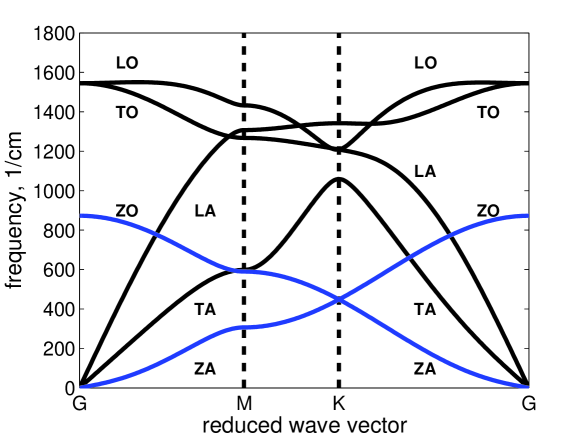
Figure 2: Calculated phonon dispersion for graphene; the force constants, elastic constants, and phonon frequencies in critical points are listed in Tables 1, 2, and 3 correspondingly.

The calculated phonon dispersion is shown in Fig. 2. Notice, first, that the sound velocities (for the long waves, $q\rightarrow\Gamma$) are isotropic in the $xy$ plane as it should be appropriate for the symmetry of graphene. Second, the in-plane LO/TO modes at $\Gamma$, the in-plane LO/LA modes at $K$, and the out-of-plane ZA/ZO modes at $K$ are doubly degenerate, because graphene is the non-polar crystal and the $C_{3v}$ symmetry of these points in the Brillouin zone admits the two-fold representation (observation of splitting of that modes in graphene would display the symmetry braking of the crystal).

III Fitting to experimental data for graphite

Because of the lack of information on graphene, we compare the present theory with experiments on graphite. In fitting to the experimental data, we must keep in mind that the frequencies in graphene for the out-of-plane branches should be less than their values in graphite, since the atoms are more free to move in the $z$ direction in graphene comparatively with graphite. It is evident that the adjacent layers in graphite affect more intensively the low frequencies. The interaction of the adjacent layers can be estimated from the observed splitting at around 130 cm^-1 [see, for instance, Ref. MM ] of the ZA and ZO’ modes which slick together if the interaction is absent.

Thus, we have only two force constants $\alpha_{z}$ and $\gamma_{z}$ to fit four Raman frequencies of the out-of-plane modes. We see also from Eq. (10) that these force constants determine the velocity $s_{z}$ of the acoustic out-of-plane mode along with the elastic constant $C_{44}$. This our result contradicts to the well-known statement DS that the acoustic out-of-plane mode has a quadratic dispersion. That can be found only if the condition $\gamma_{z}=-\alpha_{z}/6$ of the velocity vanishing is satisfied. Therefore, the force constant $\alpha_{z}$ given in Table 1 is obtained using the experimental value of the out-of-plane Raman frequency. The small force constant $\gamma_{z}$ is found from the value of $C_{44}$, Table 2, taking the experimental error into account. As one can see in Table 3, the lower frequencies of the out-of-plane mode at other critical points in graphene turn out to be less than their values in graphite. The interlayer interaction should diminish that differences. On the other hand, the fact that the sound velocity $s_{z}$ is very sensitive to the small variation of $\gamma_{z}$ and becomes complex for $\gamma_{z}>0.21\times 10^{5}$ cm^-2 indicates that graphene is nearly unstable with respect to transformation into a phase of the lower symmetry group at $\Gamma$.

For the in-plane modes, we have to fit eight Raman frequencies and two elastic constants using four force constants. The equations (II.2), (17), and (18) can be used as a starting point. Fitting of the in-plane branches is insensitive to the imaginary part of the constant $\delta$. Therefore, it is taken as a real parameter. Results of fitting are presented in Fig. 2 and in Tables. Notice, that the extent of agreement of the present theory with the data obtained for graphite corresponds to the comparison level between the first-principal calculations for graphite in Ref. MRTR and their experimental data (see Table 3). We see only qualitative discrepancy in the subsequence of the levels at M: in Fig. 2 the highest level is the LO mode, whereas in Ref. MRTR the crossover of the TO and LO modes is found out on the $\Gamma$-M line (similar to $\Gamma$-K line), yielding the TO mode higher at M. We examined versions with the crossover. The agreement with experiments is not so good in these cases as for one that shown in Fig. 2 and Tables, but the discrepancies of the order of 50 cm^-1 between the different experiments as well as the distinctions between graphene and graphite do not allow us to choose the version conclusively. The experiment on graphene would clarify this point.

IV Summary

We calculate the phonon dispersion in graphene using the Born-von-Karman model with only the first- and second-neighbor interactions imposed by the symmetry constraints. The bending (out-of-plane) modes are not coupled with the in-plane branches and indicate the latent instability of graphene with respect to transformation into a lower-symmetry phase. The Raman frequencies of these modes are less than the corresponding values in graphite. The fitting of the higher in-plane modes shows the good agreement of the calculated optical frequencies as well as elastic constants with experiments.

- (1) K.S. Novoselov et al., Science, 306, 666 (2004); K.S. Novoselov et al., Nature, 438, 197 (2005).
- (2) Y. Zhang, J.P. Small, M.E.S. Amory, P.Kim, Phys. Rev. Lett. 94, 176803 (2005).
- (3) C.C. Ferari, J.C. Meyer, V. Scardaci, C. Caseraghi, M. Lazzeri, F. Mauri, S. Piscanec, D. Jiang, K.S. Novoselov, S. Roth, and A.K. Geim, Phys. Rev. Lett. 97, 187401 (2006).
- (4) A.H. Castro Neto, F. Guinea, Phys. Rev. B 75, 045404 (2007).
- (5) J. De Launay, Solid State Phys. 3, 203 (1957).
- (6) R. Nicklow, W. Wakabayashi, and H.G. Smith, Phys. Rev. B 5, 4951 (1972).
- (7) A.A. Ahmadieh and H.A. Rafizadeh, Phys. Rev. B 7, 4527 (1973).
- (8) A.P.P. Nicholson and D.J. Bacon, J. Phys. C 10, 2295 (1977).
- (9) M. Maeda, Y. Kuramoto, and C. Horie, J. Phys. Soc. Jpn. Lett. 47, 337 (1979).
- (10) R. Al-Jishi and G. Dresselhaus, Phys. Rev. B 26, 4514 (1982).
- (11) H. Gupta, J. Malhotra, N. Rani, and B. Tripathi, Phys. Rev. B 33, 7285 (1986).
- (12) L. Lang, S. Doyen-Lang, A. Charlier, and M.F. Charlier, Phys. Rev. B 49, 5672 (1994).
- (13) J. Maultzsch, S. Reich, C. Thomsen, H. Reequardt, and P. Ordejon, Phys. Rev. Lett. 92, 075501 (2004).
- (14) M. Mohr, J. Maultzsch, E. Dobardz̆ić, I. Milos̆ević, M. Damnjanović, A. Bosak, M. Krish, and C. Thomsen, cond-mat/0705.2418, unpublished.
- (15) D. Sánchez-Portal, E. Artacho, and J.M. Soler, Phys. Rev. B 59, 12678 (1999).
- (16) O. Dubay and G. Kresse, Phys. Rev. B 67, 035401 (2003).
- (17) A. Charlier, E. McRae, M.-F. Charlier, A. Spire, and S. Forster, Phys. Rev. B 57, 6689 (1998).
- (18) A. Grüneis, R. Saito, T. Kimura, L.G. Cancado, M.A. Primenta, A. Jorio, A.G. Souza Filho, G. Dresselhaus, and M.S. Dresselhaus, Phys. Rev. B 65, 155405 (2002).
- (19) C. Mapelli, C. Castiglioni, and G. Zerbi, Phys. Rev. B 60, 12710 (1999).
- (20) V.N. Popov and P. Lambin, Phys. Rev. B 73, 085407 (2006).
- (21) R. Saito, G. Dresselhaus, and M.S. Dresselhaus, Physical Properties of Carbon Nanotubes, p. 170, (Imperial College Press, London, 1998).
- (22) N. Mounet and N. Marzari, Phys. Rev. B 71, 205214 (2005).
- (23) L. Landau and E. Lifchitz, Theory of Elasticity, p. 140, (Editions ”Nauka”, Moscow, 1987).
- (24) Graphite and Precursors, ed. by P. Delhaes (Gordon and Breach, Australia, 2001), Chap. 6.
- (25) C. Oshima, T. Aizava, R. Souda, Y. Ishizava, and Y. Samiyosh, Solid. State. Commun. 65, 1601 (1988).
- (26) H. Yanagisawa, T. Tanaka, Y. Ishida, M. Matsue, E. Rokuta, S. Otani, and C. Oshima, Surf. Interface Anal. 37, 133 (2005).