On the extrinsic piezoelectricity

Abstract

This work presents a continuation of our last paper, concerning the theory of the response of an antiparallel domain structure in a plate-like electroded sample to external electric field. The theory is based on the exact formula for free energy of the system, formed of a central ferroelectric part, isolated from electrodes (with a defined potential difference) by a surface layers. Our calculations are applicable also to thin films. It is usual to use the term ‘extrinsic’ for the contribution of domain walls displacement to macroscopic properties of a sample. In our last paper we discussed the extrinsic contribution to permittivity. In this work we concentrate on extrinsic contribution to piezoelectric coefficients in ferroelectrics which are simultaneously ferroelastics. As an example, we calculate the extrinsic contribution to $d_{36}$ piezoelectric coefficient of $\rm RbH_{2}PO_{4}$, that was recently measured in a wide range of temperature below Curie point.

I Introduction

Samples of ferroelectric single crystals often posses a surface layers. Its existence greatly influences properties of bulk samplesArtA2:102 ; ArtA2:110 ; ArtA2:94 ; ArtA2:342 as well as of thin films.ArtA2:255 Equilibrium domain structure in the system, mentioned above in the abstract, and the role of the surface layers was first discussed by Bjorkstam and OettelArtA2:625 in a special case of shorted electrodes. In our recent paperArtA2:kopal2 we reconsidered this problem in a general case of nonzero voltage between electrodes, discussing the response of the domain structure to external electric field. Our calculations are valid also for thin films and present, in fact, continuation of our discussion of domain structures of thin filmsArtA2:kopal1 .

InArtA2:kopal2 we used our theoretical results for prediction of extrinsic contribution to permittivity of the sample. In the next two sections we give a short review of notation, description of the model and basic results fromArtA2:kopal2 . In last two sections we discuss as an example the extrinsic contribution to $d_{36}$ piezoelectric coefficient of $\rm RbH_{2}PO_{4}$. We compare our predictions with the recent measurements of record values $\sim 4000\rm\,pC/N$ in temperature range 35 K under critical temperature 146 KArtA2:stula (see alsoArtA2:nakamura ).

II Description of the model

We consider a plate-like electroded sample of infinite area with major surfaces perpendicular to the ferroelectric axis $z$. Central ferroelectric part with antiparallel domains (2.) is separated from the electrodes (0.), (4.) by nonferroelectric layers (1.),(3.) (see Fig. II). The spatial distribution of the electric field $E$ is determined by the applied potential difference $V=\varphi^{(4)}-\varphi^{(0)}$ and by the bound charge div$\mbox{\boldmath$P$}_{0}$ on the boundary of ferroelectric material, where $\mbox{\boldmath$P$}_{0}$ stands for spontaneous polarization. Geometrical, electrical and material parameters of the system are shown in Fig. II.

We further introduce the symbols

$$c=\sqrt{\varepsilon_{a}/\varepsilon_{c}},\qquad g=\sqrt{\varepsilon_{a}\,\varepsilon_{c}},$$

and several geometrical parameters: the slab factor

$$B=\frac{d}{h},$$

[r][t] Geometry of the model the domain pattern factor

$$R=\frac{\pi h}{2a},\quad 2a=a_{+}+a_{-},$$

and the asymmetry factor

$$A=\frac{a_{+}-a_{-}}{a_{+}+a_{-}}\ .$$

The ferroelectric material itself is approximated by the equation of state

$$D_{x} = \varepsilon_{0}\varepsilon_{a}E_{x},$$

$$D_{z} = \varepsilon_{0}\varepsilon_{c}E_{z}+P_{0},$$

where $P_{0}$ is the spontaneous polarization along the ferroelectric axis. This linear approximation limits the validity of our calculations to the temperature region not very close below the transition temperature $T_{c}$. Domain walls are assumed to have surface energy density $\sigma_{w}$ and zero thickness.

III Gibbs electric energy of the system, equilibrium domain structure

Rather cumbersome calculationsArtA2:kopal2 lead to the following formula for Gibbs electric energy per unit area of the system (in $\rm J\,m^{-2}$), which includes the domain wall energy, the electrostatic energy whose density is $(1/2)\mbox{\boldmath$E$}\cdot(\mbox{\boldmath$D$}-\mbox{\boldmath$P$}_{0})$ and the work performed by external electric sources $-VQ$, where $Q$ is the charge on positive electrode.

$$G=\frac{2}{\pi}\sigma_{w}R+P_{0}A\ \frac{P_{0}A\,Bt-2\varepsilon_{0}\varepsilon_{d}V\left(1+B\right)}{2\varepsilon_{0}\left(1+B\right)\left(\varepsilon_{d}+B\,\varepsilon_{c}\right)}+\frac{4P_{0}^{2}t}{\varepsilon_{0}\pi^{2}R(1+B)}\sum^{\infty}_{n=1}\frac{\sin^{2}{(n\pi(1+A)/2)}}{n^{3}(\coth{nBR}+g\coth{nRc})}\ .$$ (1)

The first term represents domain wall contribution while the last one is the depolarization energy. In the second term we recognize the effect of layers (1.) and (3.) and of the applied voltage.

In this model we neglect the mechanical interactions between components of the system. For given slab factor $B$ and voltage $V$, the equilibrium domain structure, characterized by $R_{\rm eq}(V)$ and $A_{\rm eq}(V)$, corresponds to local minimum of $G$. In general a minimum can be found by numerical methods, but for $BR\gg 1$ and $Rc\gg 1$, the $R_{\rm eq}(V)$ and $A_{\rm eq}(V)$ can be approximated by explicit formulae. For purpose of this paper we use the following formula for $A_{\rm eq}(V)$

$$A_{\rm eq}(V)\cong\frac{\varepsilon_{0}V}{tP_{0}}\left[\frac{B}{\varepsilon_{d}(1+B)}-X\right]^{-1}$$ (2)

where

$$X=\frac{2\,\ln{2}\left(1+B\varepsilon_{c}/\varepsilon_{d}\right)}{R^{0}_{\rm eq}\,(1+B)(\varepsilon_{d}+\sqrt{\varepsilon_{a}\,\varepsilon_{c}})}$$

is considered as a small correction and $R^{0}_{\rm eq}$ is equilibrium value of $R$ for zero voltage $V$. For the extrinsic contribution to permittivity of the sample we get from (2) (see alsoArtA2:kopal2 )

$$\varepsilon_{\rm ext}=\left\{\left(1+B\,\frac{\varepsilon_{c}}{\varepsilon_{d}}\right)\left[\frac{B}{(1+B)\,\varepsilon_{d}}-X\right]\right\}^{-1}$$ (3)

IV Extrinsic piezoelectricity

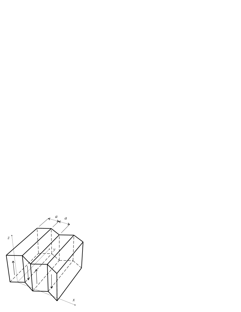
a)

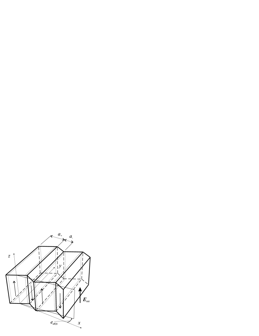
b)

Figure 1: Symmetric domain structure with spontaneous strain $e_{0,6}$, (a) $E_{\rm ext}=0,A=0$, (b) $E_{\rm ext}\neq 0,A\neq 0$

As an example, in this section we work out the approximate prediction of extrinsic contribution to $d_{36}$ of $\rm RbH_{2}PO_{4}$ (RDP), based on our simple model. RDP is a ferroelastic with spontaneous strain $e_{0,6}$, opposite in opposite polarized domains. In the Fig.1a there is $x-y$ cut through symmetric domain structure ($A=0$, $E_{\rm ext}=V/t=0$). The situation after application of $E_{\rm ext}$ is shown in Fig.1b ($A\neq 0$). A simple geometric consideration leads to the formula for average strain $e_{\rm eff,6}$ of the sample (we neglect the mechanical coupling of the central part with the rest of the sample)

$$e_{\rm eff,6}=e_{0,6}A$$ (4)

For the extrinsic coefficient $d_{36}$ we get from (2) and (4)

$$d_{36}\equiv\frac{e_{\rm eff,6}}{E_{3}}=\frac{\varepsilon_{0}e_{0,6}}{P_{0}}\,\left[\frac{B}{(1+B)\,\varepsilon_{d}}-X\right]^{-1}$$ (5)

neglecting the small $X$ and for $B\ll 1$ we get more simple formula

$$d_{36}=\frac{\varepsilon_{0}\varepsilon_{d}e_{0,6}}{P_{0}B}\ .$$ (6)

V Discussion

An extremely high $d_{36}$ under $T_{c}$ for RDP was first reported inArtA2:shuvalov . In a recent paperArtA2:sidorkin , Sidorkin deduced the dispersion law of domain wall vibrations, however, in his treatment the existence of a surface layers is not explicitly considered. We can fit our theoretical results to measured onesArtA2:stula - $d_{36,\rm ext}\doteq 4\cdot 10^{-9}\,{\rm C/N},\varepsilon_{\rm z,ext}=2000$ in the 35 K range plateau under $T_{c}$. Using values that roughly apply to RDP: in (6) resp. (3) we come to an agreement for reasonable value of $B\doteq 0.04$. Naturally for lower temperatures, the motion of the walls is limited by “freezing” and both $d_{\rm 36,ext}$ and $\varepsilon_{\rm z,ext}$ decrease to zero. It is also interesting, for measurements inArtA2:stula with alternating $E_{\rm ext}\doteq 20\,\rm V/m$, that corresponding amplitude of alternating $A$ from (2) is only $10^{-5}$ and displacement of the walls with $a\doteq 10\,\rm\mu m$ is of the order $10^{-10}\,\rm m$.

- (1) R. C. Miller and A. Savage, J. Appl. Phys. 32 (1961).
- (2) M. E. Drougard and R. Landauer, J. Appl..Phys 30 (1959).
- (3) H. E. Müser, W. Kuhn and J. Albers, Phys. Stat. Sol.(a) 49 (1978).
- (4) D. R. Callaby, J. Appl. Phys. 36 (1965).
- (5) A. K. Tagantsev, C. Pawlaczyk, K. Brooks and N. Setter, Integrated ferroelectrics 4 (1994).
- (6) J. L. Bjorkstam and R. E. Oettel, Phys. Rev. 159 (1967).
- (7) A. Kopal, P. Mokrý, J. Fousek, T. Bahnik, to appear in Ferroelectrics.
- (8) A. Kopal, T. Bahník and J. Fousek, Ferroelectrics 202 (1997).
- (9) M. Štula, J. Fousek, H. Kabelka, M. Fally and H. Warhanek, J. Kor. Phys. Soc. (Proc. Suppl.) 32 (1998).
- (10) E. Nakamura, Ferroelectrics 135 (1992).
- (11) L. A. Shuvalov, I. S. Zheludev, A. V. Mnatskanyan and Ts.-Zh. Ludupov, I. Fiala, Bull. Acad. Sci. USSR, Phys. Ser. 31 (1967).
- (12) A. S. Sidorkin, J. Appl. Phys. 83 (1998).