Transmission eigenchannels from non-equilibrium Green’s functions

Abstract

The concept of transmission eigenchannels is described in a tight-binding nonequilibrium Green’s function (NEGF) framework. A simple procedure for calculating the eigenchannels is derived using only the properties of the device subspace and quantities normally available in a NEGF calculation. The method is exemplified by visualization in real-space of the eigenchannels for three different molecular and atomic-wires.

I Introduction

Electronic transport properties of atomic-scale conductors has been investigated intensively in the last decadeAgrait et al. (2003); Cuniberti et al. (2005). Examples of interest include molecular wires connected to metal electrodes, atomic metal wires, and nanotubes. First principles transport calculations on these systems give results that are, in general, difficult to interpret due to the multi-channel nature of the scattering problem and the fact that the scattering states are generated from the atomic valence orbitals. The free-electron-type of reasoning normally used in mesoscopic quantum transport is thus not adequate. It is therefore useful to analyze the conduction in terms of eigenchannels. Eigenchannels are particular scattering states Büttiker (1988) with a well-defined transmission probability, $0\leq T_{n}\leq 1$, where the individual eigenchannel transmissions add up to the total transmission $T=\sum_{n}T_{n}$. In addition to being useful for analyzing theoretical calculations, the eigenchannel transmissions may be obtained experimentally (i) with superconducting electrodes connecting the atomic-scale conductor, as first shown by Scheer et al. Scheer et al. (1998), or (ii) from shot noise measurementsAgrait et al. (2003) where information about the individual channel contributions can be obtained since the Fano factor involve the sumAgrait et al. (2003); Blanter and Buttiker (2000) $\sum_{n}T_{n}(1-T_{n})/\sum_{n}T_{n}$.

Eigenchannels have previously been calculated for atomic metal wiresKobayashi et al. (2000); N. Lorente (2006) and molecular contactsTaylor et al. (2003) by directly solving for the scattering states in the leads. This type of analysis breaks up the transmission into the ’non-mixing’ channelsBüttiker (1988); Brandbyge et al. (1997); Cuevas et al. (1998) and gives an intuitive picture of electron transport. The ability to plot the eigenchannel wavefunctions is especially useful, since it gives a direct spatially resolved picture of the orbitals involved in the transport. Another possibility is to consider projections of eigenchannel wavefunctions onto, for example, molecular orbitals.

An increasingly popular theoretical approach to calculate transport properties is the non-equilibrium Green’s function (NEGF) formalismDatta (1995). This is normally used in combination with a tight-binding type or LCAO electronic structure descriptionBrandbyge et al. (2002); P.S. Damle and Datta (2002); Rocha et al. (2006); Palacios et al. (2002). In this approach, it is straightforward to calculate the single particle (retarded) Green’s function (matrix) including coupling to the infinite electrodes by introducing self-energies. The Green’s function is thus the fundamental quantity in these calculations and scattering states are normally not considered. Interpretation of the results in terms of scattering states is therefore non-trivialJacob and Palacios (2006). In contrast, the scattering states are the fundamental quantity in approaches based on the Lippmann-Schwinger equation where jellium models are normally used to describe the electrodesLANG (1995); Hirose and Tsukada (1995); Paulsson and Stafström (2001); Di Ventra and Lang (2002).

The aim of this paper is to show how the eigenchannels can be easily generated within the NEGF approach without solving for the scattering states in the leads. The eigenchannel wavefunctions are here obtained directly from quantities readily available in the NEGF calculation, e.g., the retarded Green’s function matrix, $G_{D}$ of the device region, and the $\Gamma_{L,R}$ matrices describing the coupling of the device region to the two electrodes (’left’ $L$ and ’right’ $R$, see Fig. 1). In the case of atomistically defined electrodes, this approach is especially advantageous since solving for the scattering states requires calculating the Bloch waves in the electrodes (complex band structure), which may be a non-trivial numerical task for large unitcellsTomfohr and Sankey (2002). Related to our approach is the so-called (left/right) open ’channel functions’ of Inglesfield an co-workers based on the ’embedding potential’ in the real-space formulationInglesfield et al. (2005), and the KKR-based formulation by Bagrets et al. Bagrets et al. ; Bagrets et al. (2006). In addition to providing a simple way to calculate the eigenchannels, the method presented here offers an intuitive understanding of the one-particle NEGF equations, e.g., it may be used to understand propensity rules for the effect of phonon scattering on the electronic transportPaulsson et al. (2005, ).

The paper is organized as follows. Sec. II starts with the definition of eigenchannels and a summary of the standard one particle NEGF equations. Our method to obtain the eigenchannels without solving for the full transmission matrix is then derived. The usefulness of the eigenchannels is illustrated in Sec. III with three examples where the eigenchannels are calculated for molecular and atomic-wires connected to gold electrodes using a first-principles density functional method.

II Eigenchannels

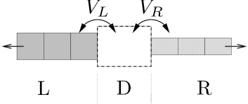
Figure 1: The generic two probe system which couples the left ($L$) and right ($R$) leads through an intermediate ”device” region ($D$).

We consider transport through a device region, $D$, coupled to two semi-infinite leads, left and right ($L,R$) and limit ourselves to leads built from periodic cells. The solutions in the corresponding infinite left/right leads are Bloch states $|u_{l}\rangle$ ($|u_{r}\rangle$) denoted by band-index $l$ ($r$) for the left (right) lead. In order to obtain the transmission amplitude matrix ${\bf t}_{r,l}$ at a given energy, $E$, we consider the solutions to the Schrödinger equation, $|\Psi_{l}\rangle$ with scattering boundary conditions and incoming waves in the left lead,

$$|\Psi_{l}\rangle= \frac{|u_{l}\rangle}{\sqrt{v_{l}}}+\text{Reflected} \mbox{; left lead},$$

$$|\Psi_{l}\rangle= \sum\limits_{r}\frac{|u_{r}\rangle}{\sqrt{v_{r}}}{\bf t}_{r,l}+\text{Decaying} \mbox{; right lead},$$ (1)

where $|u_{l}\rangle$ is an incoming Bloch wave from the left lead, i.e., right-moving, with energy $E$ and group velocity $v_{l}>0$, and $|u_{r}\rangle$ is an out-going Bloch wave ($v_{r}>0$). At a certain energy, the number of such in-coming channels, $N_{L}(E)$, is determined by the band structure of the lead. Likewise, there are $N_{R}(E)$ such out-going channels on the right. In Eq. 1, we explicitly state the flux-normalization by dividing the Bloch state by ${\sqrt{v_{l}}}$, where the Bloch waves $|u_{l}\rangle$ are normalized in the conventional manner over the infinite leads $\langle u_{l}(k)|u_{l^{\prime}}(k^{\prime})\rangle=\delta_{ll^{\prime}}\,\delta(k-k^{\prime})$ . The reflected and transmitted parts may contain evanescent decaying waves which have zero velocity and for those states we use normal integral normalization. With these considerations we find that the flux-normalized states fulfil the normalization,

$$\frac{1}{\sqrt{v_{l}}}\langle u_{l}(k)|u_{l^{\prime}}(k^{\prime})\rangle\frac{1}{\sqrt{v_{l^{\prime}}}}=\,\hbar\,\delta_{ll^{\prime}}\,\delta(E-E^{\prime})\,,$$ (2)

since the velocity is related to the energy as $v_{l}=1/\hbar\,d\varepsilon_{l}(k)/dk$. The scattering states generated from the flux-normalized incoming waves will also be flux-normalized, see Appendix A,

$$\langle\Psi_{l}|\Psi_{l^{\prime}}\rangle=\hbar\,\delta_{ll^{\prime}}\,\delta(E-E^{\prime})\,,$$ (3)

and likewise for $r,r^{\prime}$ while $\langle\Psi_{l}|\Psi_{r}\rangle=0$.

The advantage of using flux-normalized states is that we can make any unitary transformation between the incoming scattering states from the left lead at a particular energy,

$$|w_{l}\rangle=\sum_{l^{\prime}}\frac{|u_{l^{\prime}}\rangle}{\sqrt{v_{l}}}\,({\bf U}_{L})_{l^{\prime},l}\,.$$ (4)

These new states will again solve the Schrödinger equation, only contain incoming waves in the left lead, and be fluxnormalized. However, the mix of Bloch waves will no longer have Bloch symmetry. Naturally we can apply a similar transformation of the out-going right channels with ${\bf U}_{R}$. Especially we can choose the transformations $({\bf U}_{L},{\bf U}_{R})$ such that the transmission matrix ${\bf t}$ becomes a diagonal matrixBrandbyge et al. (1997), ${\bf t}_{e}$, at a specific energy

$${\bf t}_{e}={\bf U}_{R}^{\dagger}\,{\bf t}\,{\bf U}_{L}={\mbox{Diag}}\left(\sqrt{T_{1}},\sqrt{T_{2}},\ldots\right).$$ (5)

This corresponds to a singular value decomposition (SVD) of the transmission amplitude matrix, or a diagonalization of the Hermitian (left-to-right) transmission probability matrix,

$${\bf T}_{e}={\bf t}_{e}^{\dagger}{\bf t}_{e}={\bf U}_{L}^{\dagger}\,{\bf t}^{\dagger}{\bf t}\,{\bf U}_{L}={\mbox{Diag}}\left(T_{1},T_{2},\ldots\right)\,,$$ (6)

where there will be a maximum of ${\mbox{Min}}(N_{L}(E),N_{R}(E))$ non-zero, eigenvalues $0\leq T_{\alpha}\leq 1$.

The diagonalization of the transmission matrix defines the transmission eigenchannels ${|\Phi_{\alpha}\rangle}$ of the system as the unitary mix of left in-coming flux-normalized scattering states (“channels”) given by ${\bf U}_{L}$, i.e., the left eigenchannels are given by ${|\Phi_{\alpha}\rangle}=\sum\limits_{l^{\prime}}{|\Psi_{l^{\prime}}\rangle({\bf U}_{L})_{l^{\prime},\alpha}}$. The eigenchannels have the special property of being “non-mixing” in the sense that the transmission of a sum of two is the sum of individual fluxes or transmissions (equal for flux normalized states). For example, consider the alternative channels given by the scattering states defined by the two first eigenchannels as, $|u_{a}\rangle=a_{1}|\Phi_{1}\rangle+a_{2}|\Phi_{2}\rangle$, with transmission $T_{a}=|a_{1}|^{2}T_{1}+|a_{2}|^{2}T_{2}$ and similarly $|u_{b}\rangle$ with transmission $T_{b}$. Now the total transmission of $|u_{c}\rangle=|u_{a}\rangle+|u_{b}\rangle$ will be $T_{c}=T_{a}+T_{b}+I$, with the interference term $I=2\,T_{1}{\rm{Re}}(a_{1}b_{1}^{*})+2\,T_{2}{\rm{Re}}(a_{2}b_{2}^{*})$. It will thus not simply be the sum of the two transmissions, $T_{c}\neq T_{a}+T_{b}$. Since the purpose of this paper is to calculate the eigenchannels without solving for the complex band structure in the leads, we will use the fact that the eigenchannels also maximize the transmission through the device, i.e., the first eigenchannel from the left contact maximize the transmission probability over the space of incoming states from the left, the next channel maximizes the transmission while being orthogonal to the first channel etc.

In the following, we will instead of flux-normalization make use of energy-normalization $\langle\Psi_{n}(E)|\Psi_{m}(E^{\prime})\rangle=\delta_{nm}\,\delta(E-E^{\prime})$ with the trivial difference from flux-normalization being a factor $\sqrt{\hbar}$. Energy-normalization is advantageous when working with energy resolved quantities since the natural continuous quantum number for this normalization is the energy. In addition, we can interpret the energy-normalized states as a density-of-states, i.e., $|\Psi_{l}(x)|^{2}=|\langle x|\Psi_{l}\rangle|^{2}$ is the projected (local) density-of-states at $x$.

II.1 Preliminaries

The one particle Hamiltonian for the tight-binding scattering problem shown in Fig. 1 can be written

$$H=H_{0}+V=H_{L}+H_{D}+H_{R}+V_{L}+V_{R}\,,$$ (7)

where the isolated leads $H_{L,R}$ and device $H_{D}$ are coupled together by the interactions between leads and device ($V=V_{L}+V_{R}$) without any direct coupling between the leads. Using projection operators onto the device $P_{D}$ and left/right leads $P_{L,R}$ ($I=P_{L}+P_{D}+P_{R}$) we can also define $\tau_{L,R}=P_{D}V_{L,R}P_{L,R}$ where $V_{L,R}=\tau_{L,R}+\tau_{L,R}^{\dagger}$. The rest of this section provide a short summary of the standard definitions of one particle Green’s functions, self-energies and the notation we will use throughout the paperDatta (1995); Paulsson .

From the definition of the retarded Green’s function (operator) for the whole system we can find the expansion of the Green’s function in an eigenbasis, $H|\Psi_{m}(E)\rangle=E|\Psi_{m}(E)\rangle$,

$$G(E) = \left(E+i\delta-H\right)^{-1}=$$ (8)

$$= \int\limits\mathrm{d}E^{\prime}\,\sum\limits_{m}\,\frac{|\Psi_{m}(E^{\prime})\rangle\langle\Psi_{m}(E^{\prime})|}{E+i\delta-E^{\prime}}\,,$$

where the infinitesimal imaginary part $\delta=0^{+}$ ensures that the Green’s function yield the retarded response of the system. The device part of the Green’s function can further be written

$$G_{D}=\left(E+i\delta-H_{D}-\Sigma_{L}-\Sigma_{R}\right)^{-1}\,,$$ (9)

where we have introduced the self-energies, $\Sigma_{L,R}=\tau_{L,R}^{\phantom{\dagger}}g^{\phantom{\dagger}}_{L,R}\tau_{L,R}^{\dagger}$ given by the Green’s functions of the isolated leads $g_{L,R}=(E+i\delta-H_{L,R})^{-1}$. In addition to the Green’s function, the spectral functions $A(E)=i(G-G^{\dagger})$, $a_{L,R}=i(g_{L,R}-g^{\dagger}_{L,R})$, and broadening $\Gamma_{L,R}=i(\Sigma_{L,R}-\Sigma_{L,R}^{\dagger})=\tau_{L,R}a_{L,R}\tau^{\dagger}_{L,R}$ will be needed. The fact that these matrices live on different subspaces will be used repeatedly, e.g., $\Gamma_{L}=P_{D}\Gamma_{L}P_{D}$ etc.

For the scattering problem, see Fig. 1, we know that the time independent discrete Schrödinger equation has a complete set of solutions. These solutions can be divided into a continuous set of solutions $|\Psi_{n}(E)\rangle$ (where there may be several solutions at any given energy) and localized states $|\Psi^{\mathrm{Loc}}_{m}\rangle$ with energy $E^{\mathrm{Loc}}_{m}$. We use the energy as the continuous quantum number together with a discrete quantum number $n$, i.e., sub-bands. Since we are only interested in the transport properties, we will from hereon ignore localized states .

In the following, we will describe a method to determine the eigenchannel scattering states inside the device region using the information contained in $G_{D}$, $\Gamma_{L}$, and $\Gamma_{R}$. The spectral function, $A$, is a central quantity in the following discussion. It can be obtained from the expansion of the retarded Green’s function in eigenfunctions to the Hamiltonian (Eq. 8),

$$A(E) = i\left(G(E)-G^{\dagger}(E)\right)$$ (10)

$$= 2\pi\sum\limits_{n}|\Psi_{n}(E)\rangle\langle\Psi_{n}(E)|\,.$$

II.2 Scattering states from the leads

We may choose to express the solutions to the Schrödinger equation as solutions consisting of waves originating in the left or right lead. These scattering states can be generated from the spectral function as will be show here. Decomposing the spectral function of the device $A_{D}=P_{D}AP_{D}$, using Eq. (9), we find

$$A_{D} = i(G_{D}-G_{D}^{\dagger})=iG_{D}\left({G_{D}^{\dagger}}^{-1}-G_{D}^{-1}\right)G_{D}^{\dagger}$$ (11)

$$= G_{D}\Gamma_{L}G_{D}^{\dagger}+G_{D}\Gamma_{R}G_{D}^{\dagger}\,,$$

where we in the following wish to show that $A_{L,R}=G_{D}\Gamma_{L,R}G_{D}^{\dagger}$ is generated by the scattering states with incoming waves in the left (right) lead.

Viewing the coupling between device and leads as a perturbation, we can start with a set of orthogonal and normalized eigenfunctions, $|{\widetilde{u}}_{l}\rangle$, of the isolated left lead (and similarly for the right) which are totally reflected solution since they are solutions for the isolated semi-infinite leads. From these states, the full solutions $|{\Psi}_{l}\rangle$ can be generated,

$$|{\Psi}_{l}\rangle=GV_{L}|{\widetilde{u}}_{l}\rangle+|{\widetilde{u}}_{l}\rangle\,.$$ (12)

The response given by the retarded Green’s function only contains waves traveling outwards from the device region. This solution to the Schrödinger equation thus have the required property of being incoming from the left lead. In addition, the solutions are energy-normalized and orthogonal, see Appendix A.

We can then express the device part of the spectral function from the solutions generated by Eq. (12)

$$A_{L} = 2\pi\sum\limits_{l}P_{D}|{\Psi}_{l}\rangle\langle{\Psi}_{l}|P_{D}$$ (13)

$$= 2\pi\sum\limits_{l}P_{D}\left(GV_{L}|{\widetilde{u}}_{l}\rangle+|{\widetilde{u}}_{l}\rangle\right)$$

$$\left(\langle{\widetilde{u}}_{l}|+\langle{\widetilde{u}}_{l}|V_{L}^{\dagger}G^{\dagger}\right)P_{D}$$

$$= P_{D}GV_{L}a_{L}V_{L}^{\dagger}G^{\dagger}P_{D}=G_{D}^{\phantom{\dagger}}\Gamma_{L}G_{D}^{\dagger}\,,$$

where we have used Eq. (10) for the whole system and for the isolated lead. Apart from re-deriving Eq. (11) we have proven that the two parts of the device spectral function $A_{L,R}=G_{D}\Gamma_{L,R}G_{D}^{\dagger}$ are built up of scattering states originating from the respective leads. This immediately leads to the well known formula for the density matrix in non-equilibrium (excluding localized states)

$$\rho=\frac{1}{2\pi}\int\limits_{-\infty}^{\infty}\left[f_{L}(E)A_{L}(E)+f_{R}(E)A_{R}(E)\right]\;\mathrm{d}E\,,$$ (14)

where $f_{L,R}$ is the Fermi function of the leads.

II.3 Current operator

To find the eigenchannels of the system we will need the current operator. The number of electrons in lead $R$ is described by the projection operator $P_{R}$. The operator for current into $R$ is thus determined the time derivative of $P_{R}$,

$$\hat{J}_{R}=2e\dot{P}_{R}=\frac{i2e}{\hbar}[H,P_{R}]=\frac{i2e}{\hbar}(\tau_{R}^{\phantom{\dagger}}-\tau_{R}^{\dagger})\,,$$ (15)

where we have evaluated the commutator using the Hamiltonian, Eq. (7), and included a factor of $2$ for spin.

The current into lead $R$ due to the scattering state with energy $E$, $|\Psi_{l}\rangle$, originating from $L$ from the original in-coming (standing) wave $|\widetilde{u}_{l}\rangle$, can be written

$$j_{ll}=\langle\Psi_{l}|\hat{J}|\Psi_{l}\rangle\,.$$ (16)

To simplify this expression, we extract the right lead part of the wavefunction using the Lippmann-Schwinger Eq. (34), gives

$$P_{R}|\Psi_{l}\rangle=P_{R}G_{0}V|\Psi_{l}\rangle+P_{R}|\widetilde{u}_{l}\rangle=g_{R}\tau_{R}^{\dagger}|\Psi_{l}\rangle\,,$$ (17)

where all quantities are evaluated at energy $E$. The current carried by the scattering state $|\Psi_{l}\rangle$ is then given by

$$j_{ll} = \frac{i2e}{\hbar}\langle\Psi_{l}|\tau^{\phantom{\dagger}}_{R}-\tau^{\dagger}_{R}|\Psi_{l}\rangle$$ (18)

$$= \frac{i2e}{\hbar}\left(\langle\Psi_{l}|\tau_{R}g_{R}^{\phantom{\dagger}}\tau_{R}^{\dagger}|\Psi_{l}\rangle-\langle\Psi_{l}|\tau_{R}g_{R}^{\dagger}\tau_{R}^{\dagger}|\Psi_{l}\rangle\right)$$

$$= \frac{e}{\pi\hbar}\;2\pi\langle\Psi_{l}|\Gamma_{R}|\Psi_{l}\rangle\;\,.$$

Summing the current over all the orthogonal, energy-normalized scattering states originating in $L$ at the specific energy yield the net current or total transmission, and thus the Landauer formula,

$$j = \sum\limits_{l}J_{ll}=\frac{e}{\pi\hbar}\,2\pi\sum\limits_{l}\langle\Psi_{l}|\Gamma_{R}|\Psi_{l}\rangle$$

$$= \frac{e}{\pi\hbar}\,\mathrm{Tr}\left(A_{L}\Gamma_{R}\right)=\frac{e}{\pi\hbar}\,\mathrm{Tr}\left(G_{D}\Gamma_{L}G_{D}^{\dagger}\Gamma_{R}\right)\,.$$

From Eq. 18, we notice that the transmission probability for any scattering state from the left $|\Psi_{l}\rangle$ is given by $2\pi\langle\Psi_{l}|\Gamma_{R}|\Psi_{l}\rangle$. The transmission probability matrix can therefore be written

$$T_{l^{\prime}l}=2\pi\langle\Psi_{l^{\prime}}|\Gamma_{R}|\Psi_{l}\rangle\;\,,$$ (20)

since we consider energy-normalized (flux-normalized except for the factor of $\hbar$) scattering states, $|\Psi\rangle$, for which the current is equivalent with the transmission.

II.4 Scattering states in the device region

To find the eigenchannels from the left lead, $|\Phi_{l}\rangle=\sum\limits_{l^{\prime}}({\bf U}_{L})_{ll^{\prime}}|\Psi_{l^{\prime}}\rangle$, we need to diagonalize the transmission probability matrix. Since we do not, in this paper, explicitly calculate the Bloch states in the leads, we will diagonalize the transmission probability matrix in an abstract basis formed by incoming waves from the left or right lead. Another, equivalent, formulation is to find the eigenchannels by maximizing the transmission at a given energy while keeping the eigenchannels orthogonal (${\bf U}_{L}{\bf U}_{L}^{\dagger}={\bf 1}$)

$$\mathrm{max}\;2\pi\langle\Phi_{l}|\Gamma_{R}|\Phi_{l}\rangle\,.$$ (21)

The main problem in finding the eigenchannels is that we do not have access to the wavefunctions, Green’s functions or spectral functions of the entire system in a typical calculation. We therefore have to find a method using only properties from the device part of the system.

Figure 2: Overview of the different states used in this section. Note that the scattering states which are non-zero in the device subspace are all spanned by the $|\widetilde{\Psi}_{l}\rangle$ states. We can therefore find the eigenchannels by studying the wavefunctions spanned by the $|\widetilde{\chi}_{l}\rangle=P_{D}|\widetilde{\Psi}_{l}\rangle$.

We will now show that optimizing the current by varying the scattering state over space spanned by the incoming states from the left lead, $\left\{|\Psi_{l}\rangle\right\}$, is equivalent with varying over the states $|\widetilde{\chi}_{l}\rangle$ defined on the device subspace, see Fig. 2. We start by diagonalizing the device part of the spectral function from the left lead

$$A_{L}(E)=\sum\limits_{l}|\chi_{l}\rangle\lambda_{l}\langle\chi_{l}|=2\pi\sum\limits_{l}|\widetilde{\chi}_{l}\rangle\langle\widetilde{\chi}_{l}|\,,$$ (22)

where the eigenvectors on the finite device space are orthonormal $\langle\chi_{l}|\chi_{l^{\prime}}\rangle=\delta_{l,l^{\prime}}$. Each $|\widetilde{\chi}_{l}\rangle=\sqrt{\lambda_{l}/2\pi}|\chi_{l}\rangle$ with non-zero eigenvalues ($\lambda_{l}\neq 0$) is the device part of a specific state $|\widetilde{\Psi}_{l}\rangle$, i.e., $|\widetilde{\chi}_{l}\rangle=P_{D}|\widetilde{\Psi}_{l}\rangle$, where the $|\widetilde{\Psi}_{l}\rangle$ states are normalized and orthogonal linear combinations of the scattering states $|\Psi_{l}\rangle$

$$|\widetilde{\chi}_{l}\rangle = \sqrt{\frac{\lambda_{l}}{2\pi}}|\chi_{l}\rangle=\frac{1}{\sqrt{2\pi\lambda_{l}}}A_{L}(E)|\chi_{l}\rangle=$$ (23)

$$= P_{D}\sqrt{\frac{2\pi}{\lambda_{l}}}\sum\limits_{l^{\prime}}|\Psi_{l^{\prime}}\rangle\langle\Psi_{l^{\prime}}|\chi_{l}\rangle\equiv P_{D}|\widetilde{\Psi}_{l}\rangle\,,$$

(using Eq.(13)) where we have defined

$$|\widetilde{\Psi}_{l}\rangle=\sum\limits_{l^{\prime}}\sqrt{\frac{2\pi}{\lambda_{l^{\prime}}}}\langle\Psi_{l^{\prime}}|\chi_{l}\rangle|\Psi_{l^{\prime}}\rangle\equiv\sum\limits_{l^{\prime}}W_{ll^{\prime}}|\Psi_{l^{\prime}}\rangle\,.$$ (24)

This shows that the states $|\widetilde{\Psi}_{l}\rangle$ are spanned by the incoming scattering states from the left lead. We further wish to show that these states are normalized in the same manner as the original scattering states, i.e., we want to show that $W_{mn}$ is unitary

$$\sum\limits_{n}W_{mn}W^{*}_{m^{\prime}n} = \frac{2\pi}{\sqrt{\lambda_{m}\lambda_{m^{\prime}}}}\sum\limits_{n}\langle\chi_{m^{\prime}}|\Psi_{n}\rangle\langle\Psi_{n}|\chi_{m}\rangle$$ (25)

$$= \frac{1}{\sqrt{\lambda_{m}\lambda_{m^{\prime}}}}\langle\chi_{m^{\prime}}|A_{L}|\chi_{m}\rangle$$

$$= \frac{\lambda_{m}}{\sqrt{\lambda_{m}\lambda_{m^{\prime}}}}\langle\chi_{m^{\prime}}|\chi_{m}\rangle=\delta_{mm^{\prime}}\,,$$

using Eqs. (13) and (22).

In addition, any scattering state outside the space spanned by $|\widetilde{\Psi}_{n}\rangle$ are orthogonal to the device subspace. This can be seen from the fact that we can write the spectral function on the device subspace as

$$A_{L} = 2\pi\sum\limits_{l}P_{D}|\widetilde{\Psi}_{l}\rangle\langle\widetilde{\Psi}_{l}|P_{D}\hskip 28.45274pt\mbox{or as}$$ (26)

$$= 2\pi\sum\limits_{l}P_{D}|\Psi_{l}\rangle\langle\Psi_{l}|P_{D}\,.$$ (27)

Comparing the two equations reveals that $P_{D}|\Psi\rangle\langle\Psi|P_{D}$ must be zero for any $|\Psi\rangle$ which is orthogonal to the space spanned by $|\widetilde{\Psi}_{l}\rangle$.

In this section we have shown that the wavefunctions $|\widetilde{\chi}_{l}\rangle$ span the device part of any scattering state generated from lead $L$, see Fig. 2. To find the eigenchannels we can therefore maximize the current through the device with respect to a linear combination of $|\widetilde{\chi}_{l}\rangle$ instead of maximizing with respect to the full scattering states $|\Psi_{l}\rangle$. This is equivalent with diagonalizing the transmission matrix (Eq. (20)) in the basis formed by $|\widetilde{\chi}_{l}\rangle$.

II.5 Finding the eigenchannels

In general, the basis $\left\{|e_{i}\rangle\right\}$ used in a calculations is non-orthogonal with the overlap matrix defined by $\left[{\bf S}\right]_{ij}=\langle e_{i}|e_{j}\rangle$. Although the eigenchannels may be calculated directly in this non-orthogonal basis, we will make use of Lövdin ortogonalization to simplify the algebra. The ortogonalized matrices (denoted by a bar) are given by, ${\bf\bar{\Gamma}}_{R}={\bf S}^{-1/2}{\bf\Gamma}_{R}{\bf S}^{-1/2}$ and ${\bf\bar{A}}_{L}={\bf S}^{1/2}{\bf A}_{L}{\bf S}^{1/2}$ etc. The eigenchannels obtained in the Lövdin orthogonalized basis can at the end of the calculation simply be transformed back into the non-orthogonal basis for further visualization or projection.

From the previous section we learned that it is enough to diagonalize the transmission probability matrix (Eq. 20) $T_{l^{\prime}l}=2\pi\langle\widetilde{\chi}_{l^{\prime}}|\bar{\Gamma}_{R}|\widetilde{\chi}_{l}\rangle$ in the abstract basis $\left\{|\tilde{\chi}_{l}\rangle\right\}$. To transform $2\pi{\bar{\Gamma}}_{R}$ into the basis $\left\{|\widetilde{\chi}_{l}\rangle\right\}$, we first need to calculated the eigenvectors of ${\bar{A}}_{L}=\bar{G}{\bar{\Gamma}}_{L}\bar{{G}}^{\dagger}$,

$$\sum\limits_{n}\left[{\bf{\bar{A}}}_{L}\right]_{mn}\left[{\bf U}\right]_{nl}=\lambda_{l}\left[{\bf U}\right]_{ml}\,,$$ (28)

where $\bf{U}$ is unitary. We then obtain the transformation matrix to the $\left\{|\widetilde{\chi}_{l}\rangle\right\}$ basis,

$$\left[{\bf\widetilde{U}}\right]_{ml}=\sqrt{\frac{\lambda_{l}}{2\pi}}\left[{\bf U}\right]_{ml}\,,$$ (29)

which gives the explicit expression for the matrix we want to diagonalize

$$T_{l^{\prime}l}=2\pi\langle\widetilde{\chi}_{l^{\prime}}|\bar{\Gamma}_{R}|\widetilde{\chi}_{l}\rangle=2\pi\left[\widetilde{\bf{U}}^{\dagger}{\bf{\bar{\Gamma}}}_{R}\widetilde{\bf{U}}\right]_{l^{\prime}l}\,,$$ (30)

the eigenproblem is therefore

$$\sum\limits_{n}2\pi\left[\widetilde{\bf{U}}^{\dagger}{\bf{\bar{\Gamma}}}_{R}\widetilde{\bf{U}}\right]_{mn}\left[{\bf c}\right]_{n\alpha}=T_{\alpha}\left[{\bf c}\right]_{m\alpha}\,,$$ (31)

where the eigenchannel vectors, $\bf{c}_{\alpha}$, are given in the basis described by the columns of $\widetilde{\bf{U}}$, and the eigenvalues $T_{\alpha}$ are the transmission probabilities of the individual eigenchannels, $\alpha$. Finally, transforming back to the original non-orthogonal basis (from $\widetilde{\bf{U}}$-basis to the Löwdin-basis, and from Löwdin basis to normal non-orthogonal basis) we find that the eigenchannels on the device subspace are given by,

$$P_{D}|\Phi_{\alpha}\rangle=\sum\limits_{m,n}\left[{\bf{S}}^{-1/2}\widetilde{\bf{U}}\right]_{in}\left[{\bf c}\right]_{n\alpha}|{e}_{i}\rangle\,.$$ (32)

The Eqs. (28)-(32) provide a recipy for calculating the eigenchannels of a specific scattering problem using only properties available in standard NEGF calculations. In contrast to Ref. Jacob and Palacios (2006), these eigenchannels are well defined scattering states calculated without approximations on the full device subspace.

It is interesting to note that the eigenchannels (Eq. 32) are eigenvectors to $G\Gamma_{L}G^{\dagger}\Gamma_{R}$ (can be shown using the formalism presented above). This provides a simple method to obtain an idea about the eigenchannels. However, it is important to realize that the eigenchannel wave-functions calculated from Eq. 32 are energy normalized, i.e., the amplitudes are well defined and can be compared between different eigenchannels. In contrast, the eigenvectors to $G\Gamma_{L}G^{\dagger}\Gamma_{R}$ may have any normalization and it is therefore not possible to compare amplitudes between different channels. Moreover, the energy normalized scattering states Eq. 32 yield amplitudes which correspond to local density of states and are useful to plot, as will be shown in the next section.

III Eigenchannels for atomic- and molecular wires

To exemplify the method developend in the previous section we will use three different examples of atomic and molecular-wires connected to gold electrodes. Using the TranSIESTABrandbyge et al. (2002) extension of the SIESTAOrdejon et al. (1996) density functional theory (DFT) code, we have previously studied elastic and inelastic transport properties for the systems under consideration here, (i) atomic gold wiresFrederiksen et al. , the conjugated organic molecules (ii) oligo-phenylene vinylene (OPV)Paulsson et al. (2006), and (iii) oligo-phenylene ethynylene (OPE)Paulsson et al. (2006). The TranSIESTA calculations on these systems were performed using DFT in the generalized gradient approximation using the PBE functional. The semi-infinite leads connecting the device region was modeled using self-energies in the NEGF method. A more detailed description of the calculational method may be found in Ref.Frederiksen et al. .

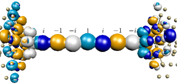
Figure 3: (Color online) Left eigenchannel for a 7-atom Au atomic chain connected by 4 atom pyramids to Au (100) surfaces. The complex phase of the eigenchannel, idicated and shown in color, is similar that of a Bloch wave at the Fermi level in the infinite atomic gold chain (half-filled 6s-band).

Gold atomic wires has been realized and studied experimentally by several different techniques. The low bias elastic and inelastic (phonon scattering) transport is well characterized and understood, see Ref.Frederiksen et al. and references therein. The first eigenchannel (from left) at the Fermi-energy is shown in Fig. 3 for a 7-atom gold chain. Not surprisingly, the majority of the transmission is carried by the first eigenchannel ($T_{1}=0.994$) with only a small transmission for the other eigenchannels ($<10^{-5}$). In addition, it is clear that the current through the wire is carried by the 6-s electrons forming a half-filled one-dimensional band where the sign of the wavefunction change by a factor of $i$ (right moving) along the wire. The only difference with the corrsponding eigenchannel from the right (not shown) is the phase factor which correcsponds to a left-moving wave.

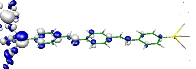
Figure 4: (Color online) Left eigenchannel for an OPV molecule bound by thiols to the hollow sites on Au (111) surfaces. The colors correspond to the two different signs of the almost real-valued wavefunction.

For molecular wires, the experimental and theoretical understanding of electron transport is less well understood. The calculated transmission through the OPV molecule shown in Fig.4 is 0.037 and $100\%$ of the transmission is carried through the first eigenchannel. Since the wave is almost totally reflected, the imaginary part of the wave-function is too small to be seen in the figure. In the calculation, the thiol bonds to the hollow site on the Au (111) surface and clearly shows that the conjugation of the molecule continues through the sulfur atom and that there is significant coupling to the gold leads.

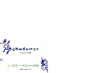
Figure 5: (Color online) Left(a) and right(b) eigenchannel for an OPE molecule strongly bound by a thiol to the left surface and weakly interacting with the right lead.

To investigate an asymmetric case, we carried out calculations on an OPE molecule bound by a thiol to the left lead, and with a tunneling barrier (hydrogen termination) to the right hand lead, see Fig. 5. The calculational details are the same as for the OPE molecule in Ref. Paulsson et al. (2006). Because of the tunneling barrier, the transmission, $T_{tot}=0.0026$, is lower than for the OPV molecule, and the left and right eigenchannels are considerably different. This can easily be understood by the large reflection at the right junction.

In the three examples described here, we find that the symmetry of the eigenchannels can be intuitively understood from the band-structure of the corresponding infinite wires. For the gold-wire, the 5d-band is below the Fermi-energy which is situated approximately at half-filling of the 6s-band. The corresponding infinite wires (polymers) for the molecular wires have energy gaps at the Fermi-energy. The eigenchannels therefore show the exponentially decaying solutions of the $\pi$-electron state in the complex-bandstructure at the Fermi-energyTomfohr and Sankey (2002).

IV Summary

We have in this paper developed a method to calculate the scattering states corresponding to elastic eigenchannels. The method is summarized in Eqs.(28)-(32) where the eigenchannels are found from quantites normally available in transport calculations using the NEGF technique. In addition, we show three brief examples of elastic scattering states calculated for molecular and atomic-wires connected to three dimensional contacts. The eigenchannels for these systems can be understood from the band-structure of the infinite wires providing an intuitive understanding.

The eigenchannels are useful to interpret elastic electron transport through junctions. We belive that they will be especially useful to investigate the effect of the contacts between device and leads, e.g., binding site of the thiol-bond on Au-surfaces. In addition, the method gives a useful basis to understand the effects of phonon scattering on the conductance and their propensity rulesPaulsson et al. (2005, ).

Appendix A Appendix: Orthogonality of scattering states

Viewing the Bloch states in the infinite, periodic leads, $|u_{l}\rangle$, as a starting point for perturbation theory, we can obtain the totally reflected solutions $|\widetilde{u_{l}}\rangle$ of a semi-infinite lead. In this case the perturbation is the removal of the coupling between the periodic cells at the surface. Furthermore, the totally reflected states may again be used as the starting point in a perturbation calculation to obtain the full scattering states $|\Psi_{l,r}\rangle$. In this case the perturbation is the device region and its coupling to the leads. We will here show that the perturbation expansion gives solutions that are orthogonal and normalized. To do this we focus on the perturbation expansion of $|\Psi_{l}\rangle$ from $|\widetilde{u_{l}}\rangle$ and note that the same derivation may be used to obtain the $|\widetilde{u_{l}}\rangle$ from $|u_{l}\rangle$.

Starting with a set of orthogonal and energy-normalized eigenfunctions $|{\widetilde{u}}_{n}(E)\rangle$ of the isolated leads ($n\in l$, $r$) we generate the full scattering states $|{\Psi}_{n}(E)\rangle$

$$|{\Psi}_{n}(E)\rangle=G(E)V|{\widetilde{u}}_{n}(E)\rangle+|{\widetilde{u}}_{n}(E)\rangle\,,$$ (33)

where $V=V_{L}+V_{R}$. The response given by the retarded Green’s function only contains waves traveling outwards from the device region. To show that the solutions generated in this way are normalized we use the Lippmann-Schwinger equation

$$|{\Psi}_{n}(E)\rangle=G_{0}(E)V|{\Psi}_{n}(E)\rangle+|{\widetilde{u}}_{n}(E)\rangle\,,$$ (34)

where the unperturbed Green’s function is $G_{0}(E)=(E-H_{L}-H_{R}-H_{D}+i\delta)^{-1}$. Together with Eq. (33), we obtain

$$\langle{\Psi}_{n}(E)|{\Psi}_{n^{\prime}}(E^{\prime})\rangle = \langle{\widetilde{u}}_{n}(E)|{\Psi}_{n^{\prime}}(E^{\prime})\rangle+\langle{\widetilde{u}}_{n}(E)|V^{\dagger}G^{\dagger}(E)|{\Psi}_{n^{\prime}}(E^{\prime})\rangle$$ (35)

$$= \langle{\widetilde{u}}_{n}(E)|{\widetilde{u}}_{n^{\prime}}(E^{\prime})\rangle+\langle{\widetilde{u}}_{n}(E)|G_{0}(E^{\prime})V^{\phantom{\dagger}}|{\Psi}_{n^{\prime}}(E^{\prime})\rangle+\langle{\widetilde{u}}_{n}(E)|V^{\dagger}G^{\dagger}(E)|{\Psi}_{n^{\prime}}(E^{\prime})\rangle$$ (36)

$$= \delta_{n,{n^{\prime}}}\delta(E-E^{\prime})+\langle{\widetilde{u}}_{n}(E)|V^{\phantom{\dagger}}|{\Psi}_{n^{\prime}}(E^{\prime})\rangle\left(\frac{1}{E^{\prime}-E+i\delta}+\frac{1}{E-E^{\prime}-i\delta}\right)$$ (37)

$$= \delta_{n,{n^{\prime}}}\delta(E-E^{\prime})\,,$$ (38)

which shows that the final scattering states $|\Psi_{n}\rangle$ are orthogonal and normalized.

References

- Agrait et al. (2003) N. Agrait, A. L. Yeyati, and J. M. van Ruitenbeek, Physics Reports 377, 81 (2003).
- Cuniberti et al. (2005) G. Cuniberti, G. Fagas, and K. Richter, Introducing Molecular Electronics (Springer, 2005).
- Büttiker (1988) M. Büttiker, IBM J. Res. Dev. 32, 63 (1988), eigenchannels are mentioned in the appendix C.
- Scheer et al. (1998) E. Scheer, N. Agrait, J. C. Cuevas, A. L. Yeyati, B. Ludoph, A. Martin-Rodero, G. R. Bollinger, J. M. van Ruitenbeek, and C. Urbina, Nature 394, 154 (1998).
- Blanter and Buttiker (2000) Y. M. Blanter and M. Buttiker, Physics Reports 336, 1 (2000).
- Kobayashi et al. (2000) N. Kobayashi, M. Brandbyge, and M. Tsukada, PHYSICAL REVIEW B 62, 8430 (2000).
- N. Lorente (2006) M. B. N. Lorente, Scanning Probe Microscopies Beyond Imaging (Wiley-VCH, 2006), chap. 15, pp. 77 – 97.
- Taylor et al. (2003) J. Taylor, M. Brandbyge, and K. Stokbro, PHYSICAL REVIEW B 68, 121101 (2003).
- Brandbyge et al. (1997) M. Brandbyge, M. R. Sørensen, and K. W. Jacobsen, Phys. Rev. B 56, 14956 (1997).
- Cuevas et al. (1998) J. C. Cuevas, A. L. Yeyati, and A. Martín-Rodero, Phys. Rev. Lett. 80, 1066 (1998).
- Datta (1995) S. Datta, Electronic Transport in Mesoscopic Systems (Cambridge University Press, Cambridge, UK, 1995).
- Brandbyge et al. (2002) M. Brandbyge, J. Mozos, P. Ordejon, J. Taylor, and K. Stokbro, PHYSICAL REVIEW B 65, 165401 (2002).
- P.S. Damle and Datta (2002) A. G. P.S. Damle and S. Datta, Chem.Phys. 281, 171 (2002).
- Rocha et al. (2006) A. R. Rocha, V. M. Garcia-Suarez, S. Bailey, C. Lambert, J. Ferrer, and S. Sanvito, Physical Review B (Condensed Matter and Materials Physics) 73, 085414 (pages 22) (2006), URL http://link.aps.org/abstract/PRB/v73/e085414.
- Palacios et al. (2002) J. J. Palacios, A. J. Pérez-Jiménez, E. Louis, E. SanFabián, and J. A. Vergés, Phys. Rev. B 66, 035322 (2002).
- Jacob and Palacios (2006) D. Jacob and J. J. Palacios, Phys. Rev. B 73, 075429 (2006).
- LANG (1995) N. LANG, PHYSICAL REVIEW B 52, 5335 (1995).
- Hirose and Tsukada (1995) K. Hirose and M. Tsukada, Phys. Rev. B 51, 5278 (1995).
- Paulsson and Stafström (2001) M. Paulsson and S. Stafström, Phys. Rev. B 64, 035416 (2001).
- Di Ventra and Lang (2002) M. Di Ventra and N. Lang, PHYSICAL REVIEW B 65, 045402 (2002).
- Tomfohr and Sankey (2002) J. K. Tomfohr and O. F. Sankey, Phys. Rev. B 65, 245105 (2002).
- Inglesfield et al. (2005) J. Inglesfield, S. Crampin, and H. Ishida, PHYSICAL REVIEW B 71, 155120 (2005).
- (23) A. Bagrets, N. Papanikolaou, and I. Mertig, cond-mat/0510073.
- Bagrets et al. (2006) A. Bagrets, N. Papanikolaou, and I. Mertig, Physical Review B 73, 045428 (2006).
- Paulsson et al. (2005) M. Paulsson, T. Frederiksen, and M. Brandbyge, Phys. Rev. B 72, 201101 (2005).
- (26) M. Paulsson, T. Frederiksen, and M. Brandbyge, in preparation.
- (27) M. Paulsson, non Equilibrium Green’s Functions for Dummies: Introduction to the One Particle NEGF equations, cond-mat/0210519.
- Ordejon et al. (1996) P. Ordejon, E. Artacho, and J. M. Soler, Phys. Rev. B 53, R10441 (1996).
- (29) T. Frederiksen, M. Paulsson, M. Brandbyge, and A.-P. Jauho, inelastic transport theory from first-principles: methodology and applications for nanoscale devices, cond-mat/0611562.
- Paulsson et al. (2006) M. Paulsson, T. Frederiksen, and M. Brandbyge, Nano Lett. 6, 258 (2006).