Multicomponent fluid of hard spheres near a wall

Abstract

The rational function approximation method, density functional theory, and NVT Monte Carlo simulation are used to obtain the density profiles of multicomponent hard-sphere mixtures near a planar hard wall. Binary mixtures with a size ratio 1:3 in which both components occupy a similar volume are specifically examined. The results indicate that the present version of density functional theory yields an excellent overall performance. A reasonably accurate behavior of the rational function approximation method is also observed, except in the vicinity of the first minimum, where it may even predict unphysical negative values.

I Introduction

Many interesting physical phenomena such as wetting and adsorption involve fluids and their mixtures at a solid-fluid interface. It is therefore not surprising that a lot of work has been devoted to these problems within the last three decades. The methods that have been used to study them include the integral equation approach of liquid state theory (see for instance Refs. HAB76 ; H78 ; PH84 ; PH85 ; HCD94 ; DAS97 ; ODHQ97 ; NHSC98 ), density functional approaches (see for instance Refs. TMvSG89 ; PH84 ; PG97 ; P99 ; RD00 ; ZR00 ; Z01 ; CG01 ) and computer simulation (see for instance Refs. SH78 ; TMvSG89 ; DH93 ; NHSC98 ; RNG05 ).

A rather simplified but essentially correct physical picture of adsorption may be obtained if one considers the solid surface as a planar smooth hard wall and the fluid as consisting of hard spheres (HS). Interestingly enough, this simple model is capable of accounting for the most important feature resulting from the interaction between the fluid particles and the wall, namely the strongly oscillatory nature of the density distribution profile of the fluid particles in the interfacial region. The particles are depleted from the surface of the wall due to excluded volume effects and this is the source of the density oscillations. A particular realization of such a model is obtained from a binary HS mixture in which one of the species is taken to have an infinite diameter and to be in vanishing concentration. In this instance, the wall-particle pair correlation functions lead immediately to the density profiles. In fact, the availability of the analytical solution of the Percus–Yevick (PY) equation for additive HS mixtures obtained by Lebowitz L64 allowed Henderson et al. HAB76 to derive the density profile of a HS fluid near a hard wall within the PY approximation already thirty years ago. More recently, Noworyta et al. NHSC98 also used the PY theory to study two binary mixtures of HS near a hard wall. In the same paper they also performed grand canonical ensemble simulations for this system and used a version of density functional theory (DFT) to derive the density profiles of both species. Their results indicated that the second order PY theory provided in general the best agreement with the simulation results and that the DFT was a little less accurate. It is interesting to point out that for the most asymmetric case that they examined, that of size ratio 1:3, anomalies were observed, namely a huge discrepancy between theory and simulation, for which they could find no explanation. This work has served as a motivation for the present paper. Here we also tackle the problem of binary HS mixtures at a planar hard wall. In addition to the PY theory, we use the results of the rational function approximation (RFA) method YSH98 , a different version of DFT mfmt , and NVT Monte Carlo simulation. Apart from complementing the work of Ref. NHSC98 , our aim is to assess the value of both the RFA method and of our version of DFT to deal with this problem in a situation where both theories are subject to rather stringent conditions, namely when there is a disparate size of the diameters but both species occupy a similar volume.

The paper is organized as follows. In order to make it self-contained, in Sec. II we provide a brief summary of the RFA method for the structural properties of a multicomponent HS mixture and state the result for the planar hard wall limit in which the concentration of one of the species goes to zero while its diameter goes to infinity. The explicit derivation of such a limit is made in the Appendix. Section III is devoted to the outline of a recent version of DFT derived by one of us mfmt . This is followed in Sec. IV by a description of the simulation details. In Sec. V we present the results derived with the two theoretical approaches as well as a comparison with the simulation data. The paper is closed in Sec. VI with further discussion and some concluding remarks.

II The Rational Function Approximation Method

We start by considering an $(N+1)$-component fluid of (additive) HS of diameters $\sigma_{i}$, mole fractions $x_{i}$ (with $i=0,1,\ldots,N$), and total bulk number density $\overline{\rho}$. The partial bulk number density of species $i$ is $\overline{\rho}_{i}=x_{i}\overline{\rho}$ and the packing fraction of the mixture is $\eta=(\pi/6)\overline{\rho}\langle\sigma^{3}\rangle$, where

$$\langle\sigma^{n}\rangle=\sum_{i=0}^{N}x_{i}\sigma_{i}^{n}$$ (1)

denotes the $n$th moment of the size distribution.

According to the RFA for HS mixtures YSH98 ; HYS07 , the Laplace transform

$$G_{ij}(s)=\int_{\sigma_{ij}}^{\infty}{\rm d}r\,e^{-sr}rg_{ij}(r)$$ (2)

of $rg_{ij}(r)$, where $g_{ij}(r)$ is the radial distribution function for the pair $ij$, is explicitly given by

$$G_{ij}(s)=\frac{e^{-\sigma_{ij}s}}{2\pi s^{2}}\left[{\sf L}(s)\cdot{\sf B}^{-1}(s)\right]_{ij},$$ (3)

where $\sigma_{ij}=(\sigma_{i}+\sigma_{j})/2$ and ${\sf L}(s)$ and ${\sf B}(s)$ are $(N+1)\times(N+1)$ matrices given by

$$L_{ij}(s)=L_{ij}^{(0)}+L_{ij}^{(1)}s+L_{ij}^{(2)}s^{2},$$ (4)

$${B}_{ij}(s)=(1+\alpha s)\delta_{ij}-{A}_{ij}(s),$$ (5)

$$A_{ij}(s) = \overline{\rho}_{i}\left[\varphi_{2}(\sigma_{i}s)\sigma_{i}^{3}L_{ij}^{(0)}+\varphi_{1}(\sigma_{i}s)\sigma_{i}^{2}L_{ij}^{(1)}\right.$$ (6)

$$\left.+\varphi_{0}(\sigma_{i}s)\sigma_{i}L_{ij}^{(2)}\right].$$

In Eqs. (4)–(6),

$$\varphi_{n}(x)\equiv x^{-(n+1)}\left(\sum_{m=0}^{n}\frac{(-x)^{m}}{m!}-e^{-x}\right),$$ (7)

$$L_{ij}^{(0)}=\lambda+\lambda^{\prime}\sigma_{j}+2\lambda^{\prime}\alpha-\lambda\sum_{k=0}^{N}\overline{\rho}_{k}\sigma_{k}L_{kj}^{(2)},$$ (8)

$$L_{ij}^{(1)}=\lambda\sigma_{ij}+\frac{1}{2}\lambda^{\prime}\sigma_{i}\sigma_{j}+(\lambda+\lambda^{\prime}\sigma_{i})\alpha-\frac{1}{2}\lambda\sigma_{i}\sum_{k=0}^{N}\overline{\rho}_{k}\sigma_{k}L_{kj}^{(2)},$$ (9)

where

$$\lambda\equiv\frac{2\pi}{1-\eta},\quad\lambda^{\prime}\equiv\frac{6\pi\eta}{(1-\eta)^{2}}\frac{\langle\sigma^{2}\rangle}{\langle\sigma^{3}\rangle}.$$ (10)

In principle, the matrix ${\sf L}^{(2)}$ and the scalar $\alpha$ can be chosen arbitrarily without violating any basic condition YSH98 ; HYS07 . In particular, the choice $L_{ij}^{(2)}=\alpha=0$ gives the PY solution L64 ; BH77 . One can go beyond this approximation by prescribing given contact values $g_{ij}(\sigma_{ij})$ and the associated thermodynamically consistent (reduced) isothermal compressibility $\chi$, what fixes ${\sf L}^{(2)}$ and $\alpha$ YSH98 ; HYS07 . Specifically,

$${L_{ij}^{(2)}}={2\pi\alpha\sigma_{ij}}g_{ij}(\sigma_{ij}),$$ (11)

while $\alpha$ is the smallest real root of an algebraic equation of degree $2(N+1)$. Here, following the method of Ref. SYH05 , we will take for $g_{ij}(\sigma_{ij})$ the following extension to mixtures of the Carnahan–Starling–Kolafa contact value K86 :

$$g_{ij}(\sigma_{ij}) = \frac{1}{1-\eta}+\frac{3\eta}{2\left(1-\eta\right)^{2}}\frac{\langle\sigma^{2}\rangle}{\langle\sigma^{3}\rangle}\frac{\sigma_{i}\sigma_{j}}{\sigma_{ij}}+\frac{\eta^{2}(5-2\eta+2\eta^{2})}{12(1-\eta)^{3}}$$

$$\times\left(\frac{\langle\sigma^{2}\rangle}{\langle\sigma^{3}\rangle}\frac{\sigma_{i}\sigma_{j}}{\sigma_{ij}}\right)^{2}+\frac{\eta^{2}(1+\eta)}{6(1-\eta)^{2}}\left(\frac{\langle\sigma^{2}\rangle}{\langle\sigma^{3}\rangle}\frac{\sigma_{i}\sigma_{j}}{\sigma_{ij}}\right)^{3}.$$

These contact values are thermodynamically consistent with Boublík’s equation of state for HS mixtures boublik . The associated (reduced) isothermal compressibility is

$$\chi = \left[\frac{1}{(1-\eta)^{2}}+\frac{6\eta}{(1-\eta)^{3}}\frac{\langle\sigma\rangle\langle\sigma^{2}\rangle}{\langle\sigma^{3}\rangle}\right.$$ (13)

$$\left.+\eta^{2}\frac{27-8\eta-8\eta^{2}+4\eta^{3}}{3(1-\eta)^{4}}\frac{\langle\sigma^{2}\rangle^{3}}{\langle\sigma^{3}\rangle^{2}}\right]^{-1}.$$

Now we assume that the mole fraction of the spheres of species $i=0$ vanishes ($x_{0}\to 0$) and that their diameter is infinitely larger than those of the other species ($\sigma_{0}/\sigma_{i}\to\infty,i\geq 1$), in such a way that $x_{0}\sigma_{0}^{n}\ll\langle\sigma^{n}\rangle$ for $n\leq 3$. In that case, species 0 does not contribute to either the total packing fraction $\eta$ or the average values $\langle\sigma\rangle$, $\langle\sigma^{2}\rangle$, and $\langle\sigma^{3}\rangle$, i.e,

$$\langle\sigma^{n}\rangle\to\sum_{i=1}^{N}x_{i}\sigma_{i}^{n},\quad n\leq 3.$$ (14)

Under those conditions a particle of species $i=0$ is seen as a planar hard wall by the $N$-component mixture made of particles of species $i=1,2,\ldots,N$. By carefully taking the limits $x_{0}\to 0$ and $\sigma_{0}\to\infty$ (with the constraint $x_{0}\sigma_{0}^{n}\ll\langle\sigma^{n}\rangle$ for $n\leq 3$), it is proven in the Appendix that the local density of particles of species $i$ at a distance $z$ from the wall is

$$\rho_{i}(z)=\overline{\rho}_{i}\gamma_{i}(z),$$ (15)

where the function $\gamma_{i}(z)$ is the inverse Laplace transform of the function defined by Eqs. (40), (42)–(46). As said in connection with Eqs. (3)–(6), (8), (9), and (11), the PY theory for $\gamma_{i}(z)$ is reobtained by setting $\alpha=0$. Our extended RFA theory is obtained by imposing Eqs. (LABEL:eCSK3) and (13) and finding the corresponding value of $\alpha$. Note that, within the RFA method, expressions for $g_{ij}$ and $\chi$ other than those of Eqs. (LABEL:eCSK3) and (13) could equally be used. The choice we have made relies on the fact that these constitute well tested and reliable approximations.

III Density functional theory

DFT is based on the property that, for a given interatomic potential, the grand potential $\Omega$, or, equivalently, the intrinsic Helmholtz free energy $F$, is a unique functional of the one-body density profile $\rho_{i}({\mathbf{r}})$ evans . For an $N$-component fluid mixture at given temperature $T$, total volume $V$, chemical potential $\mu_{i}$, and external potential $V_{i}^{\rm ext}({\mathbf{r}})$ for each component, the equilibrium density profile $\rho_{i}({\mathbf{r}})$ minimizes the grand potential functional

$$\Omega\left[\{\rho_{i}\}\right]=F\left[\{\rho_{i}\}\right]+\sum_{i=1}^{N}\int{\rm d}{\mathbf{r}}\rho_{i}({\mathbf{r}})[V_{i}^{\rm ext}({\mathbf{r}})-\mu_{i}].$$ (16)

The ideal contribution to the intrinsic free energy functional is known exactly:

$$F_{\rm id}\left[\{\rho_{i}\}\right]=k_{B}T\sum_{i=1}^{N}\int{\rm d}{\mathbf{r}}\rho_{i}({\mathbf{r}})\left\{\ln\left[\rho_{i}({\mathbf{r}})\Lambda_{i}^{3}\right]-1\right\},$$ (17)

where $k_{B}$ is the Boltzmann constant and $\Lambda_{i}$ is the thermal de Broglie wavelength of species $i$. Thus, in the task of finding the appropriate free energy functional one can focus only on the excess part

$$F_{\rm ex}\left[\{\rho_{i}\}\right]=F\left[\{\rho_{i}\}\right]-F_{\rm id}\left[\{\rho_{i}\}\right].$$ (18)

Once the expression for the intrinsic Helmholtz free energy functional is known, the density distribution is given explicitly by

$$\rho_{i}({\mathbf{r}})=\Lambda_{i}^{-3}\exp[c_{i}^{(1)}({\mathbf{r}})+\beta\mu_{i}-\beta V_{i}^{\rm ext}({\mathbf{r}})],$$ (19)

where $\beta\equiv 1/(k_{B}T)$ and $c_{i}^{(1)}({\mathbf{r}})$ is the one-body direct correlation function,

$$c_{i}^{(1)}({\mathbf{r}})=-\beta\frac{\delta F_{\rm ex}\left[\{\rho_{j}\}\right]}{\delta\rho_{i}({\mathbf{r}})}.$$ (20)

Because the knowledge of the free energy functional provides full description of the model under study, practically any implementation of DFT requires some explicit approximation for the functional $F_{\rm ex}$. In the fundamental measure theory ros , the functional $F_{\rm ex}$ of a mixture of HS is assumed to take the form

$$F_{\rm ex}\left[\{\rho_{i}\}\right]=k_{B}T\int{\rm d}{\mathbf{r}}\,\Phi(\{n_{\alpha}({\mathbf{r}})\}),$$ (21)

where the excess free energy density, $\Phi(\{n_{\alpha}({\mathbf{r}})\})$, depends only on the system averaged fundamental measures of the particles

$$n_{\alpha}({\mathbf{r}})=\sum_{i=1}^{N}\int{\rm d}{\mathbf{r}}^{\prime}\rho_{i}({\mathbf{r}}^{\prime})\omega_{i}^{(\alpha)}({\mathbf{r}}-{\mathbf{r}}^{\prime}).$$ (22)

The weight functions $\omega_{i}^{(\alpha)}({\mathbf{r}})$ characterize the geometry of particles. The minimal space of the weight functions is generated by the basis

$$\omega_{i}^{(3)}({\mathbf{r}})=\Theta(\sigma_{i}/2-r),$$ (23)

$$\omega_{i}^{(2)}({\mathbf{r}})=\delta(r-\sigma_{i}/2),$$ (24)

$$\mbox{\boldmath$\omega$}_{i}^{(2)}({\mathbf{r}})=\frac{{\mathbf{r}}}{r}\delta(r-\sigma_{i}/2),$$ (25)

where $\Theta(r)$ is the Heaviside step function and $\delta(r)$ is the Dirac delta function. The other weight functions are proportional to those given by Eqs. (23)–(25), namely $\omega_{i}^{(1)}({\mathbf{r}})=\omega_{i}^{(2)}({\mathbf{r}})/2\pi\sigma_{i}$, $\omega_{i}^{(0)}({\mathbf{r}})=\omega_{i}^{(2)}({\mathbf{r}})/\pi\sigma_{i}^{2}$, $\mbox{\boldmath$\omega$}_{i}^{(1)}({\mathbf{r}})=\mbox{\boldmath$\omega$}_{i}^{(2)}({\mathbf{r}})/2\pi\sigma_{i}$.

In this work, we apply the following form of the free energy density mfmt :

$$\Phi = -n_{0}\ln(1-n_{3})+\frac{n_{1}n_{2}-{\bf n}_{1}\cdot{\bf n}_{2}}{1-n_{3}}+(n_{2}^{3}-3n_{3}{\bf n}_{2}\cdot{\bf n}_{2})$$

$$\times\frac{8(1-n_{3})^{2}\ln(1-n_{3})+8n_{3}-(15/2)n_{3}^{2}+2n_{3}^{3}}{108\pi n_{3}^{2}(1-n_{3})^{2}}.$$

In the limit of a bulk fluid, the vectorial weighted densities ${\bf n}_{1}$ and ${\bf n}_{2}$ vanish, $n_{0}=\overline{\rho}$, $n_{1}=(\overline{\rho}/2)\langle\sigma\rangle$, $n_{2}=\pi(\overline{\rho}/2)\langle\sigma^{2}\rangle$, $n_{3}=\eta$, and therefore excess free energy density becomes equivalent to that following from Boublík’s equation of state boublik . In the low density limit the functional given by Eqs. (21) and (LABEL:Phi) is equivalent to that originally proposed by Rosenfeld, which underlies the PY compressibility solution. It is well known, however, that the PY compressibility equation of state overestimates the pressure at high densities. The functional presented here includes corrections which more accurately extrapolate from low to high density states mfmt .

In the problem at hand, the external potential represents the interaction with a planar hard wall, so that

$$V_{i}^{\rm ext}({\mathbf{r}})=\left\{\begin{array}[]{ll}\infty&{\rm for\;}z<\sigma_{i}/2\\ 0&{\rm for\;}z>\sigma_{i}/2,\end{array}\right.$$ (27)

where $z$ is the coordinate normal to the wall.

IV Simulation details

A binary mixture of HS confined in a box of dimensions $(L_{x},L_{y},L_{z})$ was simulated using the NVT Monte Carlo method. The particles were sorted out to cells and the linked-list method was used. Periodic boundary conditions were applied in the $x$ and $y$ directions, whereas flat hard walls were located at $z=0$ and $z=L_{z}$. We chose $L_{x}=L_{y}=10$ and $L_{z}=30$ in units of $\sigma_{1}$ (the diameter of the small spheres) for all the simulations.

The initial parameters of the simulations correspond to the average densities and the average concentrations. The connection between average and bulk values is not initially known so that the bulk values are evaluated in the region of the simulation box $z\sim L_{z}/2$, where no influence of the walls is expected. It is worth mentioning that the bulk values can be alternatively determined using two separate boxes connected by the same chemical potentials (one with and the other without hard walls) or using the Gibbs ensemble. However, we have found the simple NVT method (which does not involve particle insertions) to be more efficient and less problematic, especially for asymmetric mixtures and/or for high densities.

There are two common procedures as to how an initial configuration can be prepared. The random shooting method starting with the species of the largest diameter fails to converge at high packing fractions. On the other hand, the box can be initially filled up with particles placed at the crystal configuration, usually an fcc lattice. The disadvantage of the latter is the need of “relaxing” the system, a process that may take too long and may even turn to be untractable. We present a novel method which suffers none of the above mentioned problems and can be easily generalized to the model of an arbitrary number of components. First of all, both “large” and “small’ particles are inserted randomly into the box with the only restriction of no overlapping of the like particles. Then the system is left to propagate keeping the interaction between the like particles hard, whereas the penetrability of the unlike particles is restricted by the potential

$$u_{ij}(r)=\left\{\begin{array}[]{ll}\epsilon\left[1+a(\sigma_{ij}-r)/\sigma_{1}\right]&{\rm for\;}r<\sigma_{ij}\\ 0&{\rm for\;}r>\sigma_{ij},\end{array}\right.$$ (28)

where the value $a=1$ of the constant turned up to be convenient. Choosing the initial reduced temperature (typically $T^{*}\equiv k_{B}T/\epsilon=0.05$), the system was gradually cooled down. We found this algorithm to be extremely efficient in creating a non-overlapping configuration (typically within one minute using a standard PC).

The system is subsequently equilibrated over more than $10^{7}$ MC steps and the bulk densities and density profiles are averaged over another $4\times 10^{8}$ moves. The average runs were divided into $20$ subaverages to estimate the standard deviations.

V Results

Figure 1: (Color online) Density profiles close to the wall for both species in the binary HS mixtures with $\sigma_{2}/\sigma_{1}=3$ having a total packing fraction close to $\eta=0.2$. Top panels: $\eta=0.208$ and $x_{2}=0.063$; middle panels: $\eta=0.207$ and $x_{2}=0.042$; bottom panels: $\eta=0.206$ and $x_{2}=0.021$. Solid lines: DFT; dashed lines: RFA results, dash-dotted lines: PY theory. The symbols are the results of simulation. The insets provide a wider range and more details of the resulting structure.

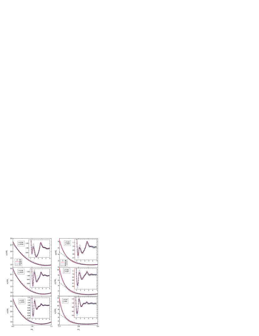
Figure 2: (Color online) The same as Fig. 1 but with a total packing fraction close to $\eta=0.3$. Top panels: $\eta=0.309$ and $x_{2}=0.062$; middle panels: $\eta=0.308$ and $x_{2}=0.037$; bottom panels: $\eta=0.307$ and $x_{2}=0.020$.

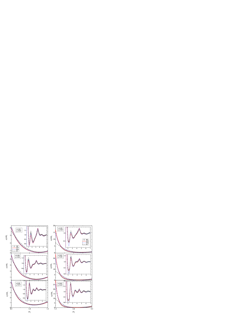
Figure 3: (Color online) The same as Fig. 1 but with a total packing fraction close to $\eta=0.4$. Top panels: $x_{2}=0.062$ and $\eta=0.401$; middle panels: $x_{2}=0.036$ and $\eta=0.406$; bottom panels: $x_{2}=0.019$ and $\eta=0.404$.

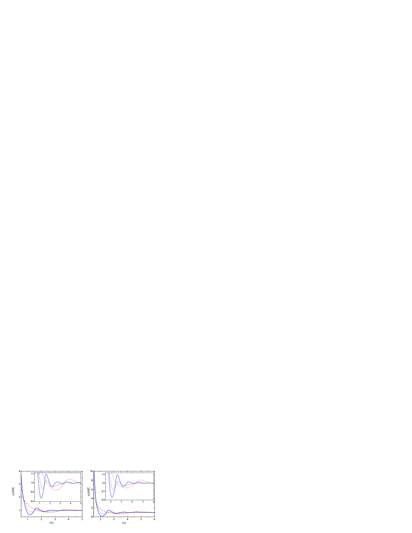
Figure 4: (Color online) Density profiles close to the wall for both species in the binary HS mixtures with $\sigma_{2}/\sigma_{1}=3$ having a total packing fraction $\eta=0.3$, as predicted by the RFA. Dashed lines: $x_{2}=\frac{10}{37}\simeq 0.27$ ($\eta_{1}/\eta_{2}=0.1$); dotted lines: $x_{2}=\frac{1}{28}\simeq 0.036$ ($\eta_{1}/\eta_{2}=1$); solid lines: $x_{2}=\frac{1}{271}\simeq 0.0037$ ($\eta_{1}/\eta_{2}=10$). The insets provide a more detailed view of the oscillations.

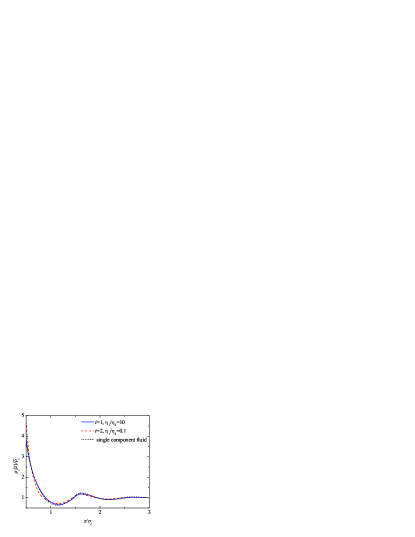
Figure 5: (Color online) Density profiles close to the wall in the binary HS mixtures with $\sigma_{2}/\sigma_{1}=3$ having a total packing fraction $\eta=0.3$, as predicted by the RFA. Solid line: $\rho_{1}(z)/\bar{\rho}_{1}$ versus $z/\sigma_{1}$ for $x_{2}=\frac{1}{271}\simeq 0.0037$ ($\eta_{1}/\eta_{2}=10$); dashed line: $\rho_{2}(z)/\bar{\rho}_{2}$ versus $z/\sigma_{2}$ for $x_{2}=\frac{10}{37}\simeq 0.27$ ($\eta_{1}/\eta_{2}=0.1$). The dotted line corresponds to the single component case.

In this Section we report the results we have obtained with the previous approaches, namely the RFA method, DFT, and simulation, for the density profiles of binary HS mixtures in the presence of a planar hard wall. In order to test the theories under extreme conditions, we consider cases in which the sizes of the two components in the mixture are disparate but both occupy a similar volume.

For the sake of illustration, in Figs. 1–3 we present the density profiles for both components of nine binary mixtures with a common size ratio $\sigma_{2}/\sigma_{1}=3$ and a total (bulk) packing fraction $\eta\simeq 0.2$ (Fig. 1), $\eta\simeq 0.3$ (Fig. 2), and $\eta\simeq 0.4$ (Fig. 3). For each packing fraction, three different compositions have been considered: $x_{2}\simeq 0.06$, so that $\eta_{2}/\eta_{1}\simeq 1.7$ (top panels); $x_{2}\simeq 0.04$, so that $\eta_{2}/\eta_{1}\simeq 1.1$ (middle panels); and $x_{2}\simeq 0.02$, so that $\eta_{2}/\eta_{1}\simeq 0.55$ (bottom panels). Here, $\eta_{i}=(\pi/6)\overline{\rho}_{i}\sigma_{i}^{3}$ ($i=1,2$) denotes the partial (bulk) packing fraction of species $i$. Since $\eta$ and $x_{2}$ are measured in the bulk, they present minor deviations with respect to the imposed average values in each case. Apart from the simulation data and our theoretical approaches, the figures also include the PY results.

Without any doubt, the DFT is the one that produces the best overall agreement. As far as the RFA method is concerned, one finds that it also does a very good job in general, being particularly accurate not only at the contact value (which is of course an input in this approach), but also caters very well for the second maximum and the rest of the oscillations. These nice features worsen in the vicinity of the first minimum, particularly for the density profile of the bigger species at $\eta\simeq 0.4$, where the RFA method may lead to the unphysical prediction of a negative value. As expected, the PY theory yields poorer contact values and gets worse as the total packing fraction increases, yielding a negative value for the first minimum of $\rho_{2}(z)$ at $\eta\simeq 0.4$ and $x_{2}\simeq 0.02$. In any case, it indeed accounts for the oscillatory character of the profiles.

Figures 1–3 show that a rich and complex structure of the local densities $\rho_{1}(z)$ and $\rho_{2}(z)$ appears for all the cases considered. This is related to the fact that $\eta_{1}\sim\eta_{2}$ and so both species compete for the available volume. As the total density increases so does the nonuniformity of the density profiles, as reflected by the contrast between the values at contact and at the first minimum, especially in the case of the large spheres. Moreover, as the mole fraction $x_{2}$ of the large spheres decreases, the characteristic wavelength of the oscillations decreases. To better understand this phenomenon, imagine a mixture with a mole fraction $x_{2}$ such that $\eta_{1}\ll\eta_{2}$. In that case, the large spheres (species 2) are practically unaffected by the presence of the small ones, so the local density $\rho_{2}(z)$ is the same as that of a single component fluid at the same packing fraction and oscillates with a characteristic wavelength of the order of $\sigma_{2}$. As for the small spheres (species 1), their density profile is dominated by the presence of the large spheres and so the wavelength of $\rho_{1}(z)$ is also of the order of $\sigma_{2}$. In the other extreme situation, namely when $\eta_{2}\ll\eta_{1}$, we have the opposite situation: the small spheres behave as a single component fluid and enslave the density profile of the large spheres, so that both $\rho_{1}(z)$ and $\rho_{2}(z)$ oscillate with a characteristic wavelength of the order of $\sigma_{1}$. The interplay between both extreme cases occurs when $\eta_{1}\sim\eta_{2}$, giving rise to the superposition of both length scales, as observed in Figs. 1–3. To illustrate the transition from $\eta_{1}\ll\eta_{2}$ to $\eta_{2}\ll\eta_{1}$, in Fig. 4 we plot the density profiles predicted by the RFA for mixtures with $\sigma_{2}/\sigma_{1}=3$, $\eta=0.3$, and $x_{2}=\frac{10}{37}\simeq 0.27$ (which corresponds to $\eta_{1}/\eta_{2}=0.1$), $x_{2}=\frac{1}{28}\simeq 0.036$ (which corresponds to $\eta_{1}/\eta_{2}=1$), and $x_{2}=\frac{1}{271}\simeq 0.0037$ (which corresponds to $\eta_{1}/\eta_{2}=10$). A ratio 1:10 in the partial packing fractions is enough to make the species with the largest packing fraction to behave almost as a single component fluid. In fact, Fig. 5 shows that the curve of $\rho_{2}(z)/\overline{\rho}_{2}$ in the case $x_{2}=\frac{10}{37}\simeq 0.27$ ($\eta_{1}/\eta_{2}=0.1$) and the curve of $\rho_{1}(z)/\overline{\rho}_{1}$ in the case $x_{2}=\frac{1}{271}\simeq 0.0037$ ($\eta_{1}/\eta_{2}=10$) look like very similar when each one is plotted as a function of the corresponding scaled distance $z/\sigma_{i}$. It must be noticed that, as observed in Fig. 5, the case $\eta_{1}/\eta_{2}=10$ is actually closer to the single component fluid than the case $\eta_{1}/\eta_{2}=0.1$. In the latter case one has $x_{1}/x_{2}=2.7$, $x_{1}\sigma_{1}/x_{2}\sigma_{2}=0.9$, and $x_{1}\sigma_{1}^{2}/x_{2}\sigma_{2}^{2}=0.3$, so that the influence of the species 1 is not entirely negligible. On the other hand, the ratios are $x_{2}/x_{1}=0.0037$, $x_{2}\sigma_{2}/x_{1}\sigma_{1}=0.011$, and $x_{2}\sigma_{2}^{2}/x_{1}\sigma_{1}^{2}=0.033$ in the case $\eta_{1}/\eta_{2}=10$.

VI Concluding Remarks

The results presented in the preceding Section deserve some further discussion. To begin with, inspired by the work of Noworyta et al. NHSC98 , we have revisited the problem of determining the structure of binary HS mixtures in the presence of a planar hard wall using three of the different approaches that have been proposed in the literature to deal with it. Concerning the RFA method, its main advantage is that of allowing for a completely analytical description, as it also occurs with the PY theory, avoiding at the same time the thermodynamic inconsistency problem present in the latter. It is fair to say that, under the rather extreme conditions that we tested it, this method is a reasonable compromise between accuracy and simplicity. Whether the difficulties associated with the prediction of a negative first minimum of $\rho_{2}(z)$ at $\eta\simeq 0.4$ and $x_{2}\lesssim 0.04$ could be avoided by the introduction of additional parameters in the method remains to be assessed. It should be mentioned in passing that for mixtures with $\eta\simeq 0.3$ this unphysical behavior is not predicted, even for $x_{2}\to 0$. Moreover, in the case of pure ternary mixtures, the agreement between the results for the structural properties of the RFA method and simulation has been shown to be highly satisfactory MMYSH02 . Finally, although we have illustrated the results for the case of binary mixtures, a further asset of the development we have presented applies in principle to any multicomponent mixture of HS near a planar hard wall. On the other hand, the excellent performance of the DFT in the approximation introduced in Ref. mfmt has been already pointed out. However the merit of the proposed excess free energy functional cannot be overlooked and might be useful for other purposes as well. As a final point, it should be stressed that the simulation method reported in this paper is also novel and allowed us to obtain results for situations that were problematic ten years ago. In particular, it allowed us to confirm the assertion made by Roth and Dietrich RD00 concerning the non existence of the anomaly reported by Noworyta et al. NHSC98 for the mixture with size ratio 1:3. Our hope and expectation is that this method proves useful as well for other interesting systems, some of which we plan to examine in the future.

Before closing this paper and for the sake of setting a wider perspective for the results we have presented, a few further comments are in order. A simple and yet realistic model of colloidal dispersions consists of a highly asymmetric binary hard-sphere mixture in which the large spheres stand for the colloidal particles and the small spheres represent solvent or polymer molecules. Therefore, our results may also be applied in these systems, which are nowadays easily amenable for experimental examination, and open up the possibility of investigating solvation forces and other interesting physical phenomena associated with particles of different sizes competing for interfacial positions in the presence of walls. We plan to pursue some of these issues in the future. On the other hand, the possible extension of our work to deal with non-hard particles remains to be explored. In the case of the RFA method, structural properties of sticky hard-sphere mixtures and other systems have already been derived HYS07 . As for the DFT approach, modifications would be required. Thus it seems that much work remains to be done before such extensions become a reality. Again, we plan to explore these and other possibilities in future studies.

Appendix A The wall limit in the RFA

The limit $x_{0}\to 0$ implies that the row $i=0$ of the $(N+1)\times(N+1)$ matrix ${\sf A}$ defined by Eq. (6) vanishes, so that

$$A_{ij}=\widetilde{A}_{ij}(1-\delta_{i0})(1-\delta_{j0})+A_{i0}(1-\delta_{i0})\delta_{j0}.$$ (29)

Here, $\widetilde{A}_{ij}$ is a projected $N\times N$ matrix with $i,j\geq 1$. In fact, $\widetilde{A}_{ij}$ is the matrix corresponding to an $N$-component mixture in the absence of species $0$. Inserting (29) into Eq. (5), we have

$$B_{ij}=\widetilde{B}_{ij}(1-\delta_{i0})(1-\delta_{j0})+(1+\alpha s)\delta_{i0}\delta_{j0}-A_{i0}(1-\delta_{i0})\delta_{j0},$$ (30)

where $\widetilde{B}_{ij}$ is the $N\times N$ matrix

$$\widetilde{B}_{ij}=(1+\alpha s)\delta_{ij}-\widetilde{A}_{ij},\quad i,j\geq 1.$$ (31)

It can be checked that the $(N+1)\times(N+1)$ inverse matrix ${\sf B}^{-1}$ is

$$\left({\sf B}^{-1}\right)_{ij} = \left(\widetilde{\sf B}^{-1}\right)_{ij}(1-\delta_{i0})(1-\delta_{j0})+(1+\alpha s)^{-1}\delta_{i0}\delta_{j0}$$ (32)

$$-C_{i}(1-\delta_{i0})\delta_{j0},$$

where $\widetilde{\sf B}^{-1}$ is the $N\times N$ inverse matrix of $\widetilde{\sf B}$ and the elements $C_{i}$ are

$$C_{i}=\frac{1}{1+\alpha s}\sum_{j=1}^{N}\left(\widetilde{\sf B}^{-1}\right)_{ij}A_{j0}.$$ (33)

Insertion of Eq. (32) into Eq. (3) yields

$$2\pi s^{2}e^{\sigma_{ij}s}G_{ij} = \sum_{k=1}^{N}L_{ik}\left(\widetilde{\sf B}^{-1}\right)_{kj}(1-\delta_{j0})+\frac{L_{i0}}{1+\alpha s}\delta_{j0}$$ (34)

$$+\sum_{k=1}^{N}L_{ik}C_{k}\delta_{j0}.$$

In particular, if $i,j\geq 1$,

$$2\pi s^{2}e^{\sigma_{ij}s}G_{ij}=\sum_{k=1}^{N}L_{ik}\left({\sf B}^{-1}\right)_{kj},\quad i,j\geq 1,$$ (35)

where we have taken into account that $\left(\widetilde{\sf B}^{-1}\right)_{ij}=\left({\sf B}^{-1}\right)_{ij}$ if $i,j\geq 1$. Equation (34) implies that, as expected, the $N$-component mixture is not affected by the presence of the species 0 in the infinite dilution limit $x_{0}\to 0$. On the other hand, setting $i\geq 1$ and $j=0$ in Eq. (34), we have

$$2\pi s^{2}e^{\sigma_{i0}s}G_{i0}=\frac{L_{i0}}{1+\alpha s}+\frac{2\pi s^{2}}{1+\alpha s}\sum_{j=1}^{N}e^{\sigma_{ij}s}G_{ij}A_{j0},\quad i\geq 1,$$ (36)

where use has been made of Eqs. (33) and (35). The cross function $G_{i0}$ (with $i=1,\ldots,N$) is related to the spatial correlation between the diluted species $0$ and the species $i$ of the true $N$-component mixture. We see from Eq. (36) that $G_{i0}$ is expressed in terms of the matrix $G_{ij}$ of the $N$-component mixture and the cross elements $L_{i0}$ and $A_{j0}$.

Let us now introduce the shifted radial distribution function

$$\gamma_{i}(z)=g_{i0}(z+\sigma_{0}/2),$$ (37)

where $z\geq\sigma_{i}/2$ represents the distance from the center of a sphere of species $i$ to the surface of a sphere of species $0$. In Laplace space,

$$G_{i0}(s)=e^{-\sigma_{0}s/2}\left[\frac{\sigma_{0}}{2}\Gamma_{i}(s)-\Gamma^{\prime}_{i}(s)\right],$$ (38)

where

$$\Gamma_{i}(s)=\int_{\sigma_{i}/2}^{\infty}{\rm d}z\,e^{-sz}\gamma_{i}(z)$$ (39)

is the Laplace transform of $\gamma_{i}(z)$ and $\Gamma^{\prime}_{i}(s)={\rm d}\Gamma_{i}(s)/{\rm d}s$.

Thus far, the diameter $\sigma_{0}$ is arbitrary as long as Eq. (14) is satisfied. Now we take the wall limit ($\sigma_{0}\to\infty$). In that case, the function $\gamma_{i}(z)$ has a clear meaning as the ratio between the local density of particles of species $i$ at a distance $z$ from the wall, $\rho_{i}(z)$, and the corresponding density in the bulk, $\overline{\rho}_{i}=\rho_{i}(\infty)$. In the wall limit $\Gamma_{i}^{\prime}(s)$ can be neglected versus $\sigma_{0}\Gamma_{i}(s)$ in Eq. (38). Therefore,

$$\Gamma_{i}(s) = {2}\lim_{\sigma_{0}\to\infty}{\sigma_{0}}^{-1}e^{\sigma_{0}s/2}G_{i0}(s)$$ (40)

$$= e^{-\sigma_{i}s/2}\left[\frac{\mathcal{L}_{i0}(s)}{\pi s^{2}(1+\alpha s)}+\frac{2}{1+\alpha s}\right.$$

$$\times\left.\sum_{j=1}^{N}e^{\sigma_{ij}s}G_{ij}(s)\mathcal{A}_{j0}(s)\right],\quad i\geq 1,$$

where in the last step use has been made of Eq. (36) and

$$\mathcal{L}_{i0}(s)\equiv\lim_{\sigma_{0}\to\infty}\sigma_{0}^{-1}L_{i0}(s),\quad\mathcal{A}_{i0}(s)\equiv\lim_{\sigma_{0}\to\infty}\sigma_{0}^{-1}A_{i0}(s).$$ (41)

From Eqs. (4), (6), (8), (9), and (11) one gets

$$\mathcal{L}_{i0}(s)=\mathcal{L}_{i0}^{(0)}+\mathcal{L}_{i0}^{(1)}s+\mathcal{L}_{i0}^{(2)}s^{2},$$ (42)

$$\mathcal{L}_{i0}^{(0)}=\lambda^{\prime}-\pi\alpha\lambda\sum_{j=1}^{N}\overline{\rho}_{j}\sigma_{j}g_{j0}(\sigma_{j0}),$$ (43)

$$\mathcal{L}_{i0}^{(1)}=\frac{\lambda}{2}+\frac{\lambda^{\prime}}{2}\sigma_{i}-\pi\alpha\frac{\lambda}{2}\sigma_{i}\sum_{j=1}^{N}\overline{\rho}_{j}\sigma_{j}g_{j0}(\sigma_{j0}),$$ (44)

$$\mathcal{L}_{i0}^{(2)}=\pi\alpha g_{i0}(\sigma_{i0}),$$ (45)

$$\mathcal{A}_{i0}(s) = \overline{\rho}_{i}\left[\varphi_{2}(\sigma_{i}s)\sigma_{i}^{3}\mathcal{L}_{i0}^{(0)}+\varphi_{1}(\sigma_{i}s)\sigma_{i}^{2}\mathcal{L}_{i0}^{(1)}\right.$$ (46)

$$\left.+\varphi_{0}(\sigma_{i}s)\sigma_{i}\mathcal{L}_{i0}^{(2)}\right].$$

It must be noted that the parameter $\alpha$ appearing in Eqs. (40) and (43)–(45) is independently obtained from the RFA solution for the $N$-component mixture. Regarding the contact values $g_{i0}(\sigma_{i0})$, they are obtained by taking the limit $\sigma_{0}\to\infty$ in Eq. (LABEL:eCSK3), namely

$$g_{i0}(\sigma_{i0}) = \frac{1}{1-\eta}+\frac{3\eta}{\left(1-\eta\right)^{2}}\frac{\langle\sigma^{2}\rangle}{\langle\sigma^{3}\rangle}{\sigma_{i}}+\frac{\eta^{2}(5-2\eta+2\eta^{2})}{3(1-\eta)^{3}}$$

$$\times\left(\frac{\langle\sigma^{2}\rangle}{\langle\sigma^{3}\rangle}{\sigma_{i}}\right)^{2}+\frac{4\eta^{2}(1+\eta)}{3(1-\eta)^{2}}\left(\frac{\langle\sigma^{2}\rangle}{\langle\sigma^{3}\rangle}{\sigma_{i}}\right)^{3}.$$

Taking into account that $G_{ij}(s)=s^{-2}+{\cal O}(s^{0})$ for small $s$, it is possible to prove that

$$\lim_{s\to 0}s\Gamma_{i}(s)=1,$$ (48)

which implies the physical condition

$$\lim_{z\to\infty}\gamma_{i}(z)=1.$$ (49)

References

- (1) D. Henderson, F. F. Abraham, and J. A. Barker, Mol. Phys. 31, 1291 (1976).
- (2) D. Henderson, J. Chem. Phys. 68, 780 (1978).
- (3) M. Plischke and D. Henderson, J. Chem. Phys. 83, 6544 (1984).
- (4) M. Plischke and D. Henderson, J. Chem. Phys. 84, 2846 (1985).
- (5) D. Henderson, K.-Y. Chan, and L. Degrève, J. Chem. Phys. 101, 6975 (1994).
- (6) R. Dickman, P. Attard, and V. Simonian, J. Chem. Phys. 107, 205 (1997).
- (7) W. Olivares-Rivas, L. Degrève, D. Henderson, and J. Quintana, J. Chem. Phys. 106, 8160 (1997).
- (8) J. Noworyta, D. Henderson, S. Sokołowski, and K.-Y. Chan, Mol. Phys. 95, 415 (1998).
- (9) Z. Tan, U. Marini Bettolo Marconi, F. van Swol, and K. E. Gubbins, J. Chem. Phys. 90, 3704 (1989).
- (10) C. N. Patra and S. K. Ghosh, J. Chem. Phys. 106, 2762 (1997); 116, 8509 (2002); 116, 9845 (2002); 117, 8933 (2002); 118, 3668 (2003).
- (11) C. N. Patra, J. Chem. Phys. 111, 6573 (1999).
- (12) R. Roth and S. Dietrich, Phys. Rev. E 62, 6926 (2000).
- (13) S. Zhou and E. Ruckenstein, J. Chem. Phys. 112, 5242 (2000).
- (14) S. Zhou, Phys. Rev. E 63, 061206 (2001).
- (15) N. Choudhury and S. K. Ghosh, J. Chem. Phys. 114, 8530 (2001).
- (16) I. K. Snook and D. Henderson, J. Chem. Phys. 68, 2134 (1978).
- (17) L. Degrève and D. Henderson, J. Chem. Phys. 100, 1606 (1993).
- (18) M. Rottereau, T. Nicolai, and J. C. Gimel, Eur. Phys. J. E. 18, 37 (2005).
- (19) J. L. Lebowitz, Phys. Rev. 133, 895 (1964).
- (20) S. B. Yuste, A. Santos, and M. López de Haro, J. Chem. Phys. 108, 3683 (1998).
- (21) Al. Malijevský, J. Chem. Phys. 125, 194519 (2006).
- (22) M. López de Haro, S. B. Yuste, and A. Santos, “Alternative Approaches to the Equilibrium Properties of Hard-Sphere Liquids,” in Playing with Marbles: Theory and Simulation of Hard-Sphere Fluids and Related Systems, edited by A. Mulero (Springer, to be published); preprint arXiv:0704.0157 [cond-mat.stat-mech].
- (23) L. Blum and J. S. Høye, J. Phys. Chem. 81, 1311 (1977).
- (24) A. Santos, S. B. Yuste, and M. López de Haro, J. Chem. Phys. 123, 234512 (2005); M. López de Haro, S. B. Yuste, and A. Santos, Mol. Phys. 104, 3461 (2006).
- (25) The Carnahan–Starling–Kolafa equation of state for a single component HS fluid is a slight modification, proposed by Kolafa, of the celebrated Carnahan–Starling equation of state. It first appeared as Eq. (4.46) in the review paper by T. Boublík and I. Nezbeda, Coll. Czech. Chem. Commun. 51, 2301 (1986).
- (26) T. Boublík, Mol. Phys. 59, 371 (1986).
- (27) R. Evans, in Inhomogeneous Fluids, edited by D. Henderson, (Dekker, New York, 1992), p 85.
- (28) Y. Rosenfeld, Phys. Rev. Lett. 63, 980 (1989).
- (29) Al. Malijevský, A. Malijevský, S. B. Yuste, A. Santos, and M. López de Haro, Phys. Rev. E 66, 061203 (2002).