Finite-well potential in the 3D nonlinear Schrödinger equation: Application to Bose-Einstein condensation

Abstract

Using variational and numerical solutions we show that stationary negative-energy localized (normalizable) bound states can appear in the three-dimensional nonlinear Schrödinger equation with a finite square-well potential for a range of nonlinearity parameters. Below a critical attractive nonlinearity, the system becomes unstable and experiences collapse. Above a limiting repulsive nonlinearity, the system becomes highly repulsive and cannot be bound. The system also allows nonnormalizable states of infinite norm at positive energies in the continuum. The normalizable negative-energy bound states could be created in BECs and studied in the laboratory with present knowhow.

1 Introduction

The nonlinear Schrödinger (NLS) equation with cubic or Kerr nonlinearity appears in many areas of physics and mathematics 1 . Of these, two areas have drawn much attention in recent time. They are pulse propagation in nonlinear medium 0a ; 3DNLS and Bose-Einstein condensation (BEC) in confining traps 8 . A quantum-mechanical mean-field description of BEC is done using the nonlinear Gross-Pitaevskii (GP) equation which is essentially the NLS equation with cubic nonlinearity. Though the NLS equation in these two areas have similar mathematical structure, the interpretation of the different terms in it is quite distinct. In BEC it is an extension of the Schrödinger equation to include a nonlinear interaction among bosons. In optics it describes electromagnetic pulse propagation in a nonlinear medium. Also, usually there is no external potential in the NLS equation in optics 1 , whereas in BEC a trapping potential is to be included in it 8 . In most studies in BEC an infinite parabolic harmonic potential has been included in the NLS equation which simulates the infinite or nearly infinite experimental parabolic magnetic trap.

In this paper we consider a finite square-well trapping potential in the NLS equation with cubic nonlinearity. Although, we consider a square-well potential for obvious analytical knowledge about this potential, most of our results should be valid for any finite potential and the experiments are really carried out on finite traps. This potential is piecewise constant and leads to analytic solution in many one-dimensional (1D) problems, and serves as a model for a trap of finite depth and can be realized in the laboratory. Because of these features, there have been several studies of the 1D NLS equation with a finite square-well and other simple potentials. Zakharov and Shabat 0a found the solutions to the NLS equation with a constant potential on the infinite line. Carr et al. solved the NLS equation under periodic and box boundary conditions c1 as well as with the 1D square-well potential c2 . There have been studies of the step function step ; step2 , point-like impurity potential pt and the parabolic potential para in the NLS equation, as well as transmission of matter wave across various potentials tr .

We extend the above 1D investigations to the spherically-symmetric three-dimensional (3D) square-well interaction. This is possibly the most-studied problem in linear quantum mechanics and allows analytic or quasi-analytic treatment in many cases. Also, it models an experimental situation which can be realized with present-day BEC technology with the use of a detuned laser beam of finite intensity c2 ; step2 . Such an optical device could generate a square-well potential in one direction c2 . Three such potentials in orthogonal directions could make an excellent model for a finite 3D square-well potential. In BEC three standing-wave orthogonal laser beams have already been used to make a 3D periodic optical-lattice potential ol . In view of this, the creation of a 3D square-well potential seems possible. Once a BEC is materialized in a square-well potential, it could be studied in the laboratory and the results compared with the prediction of the theoretical models based on the GP equation, thus providing stringent tests for these models.

We show that it is possible to have normalizable stationary BEC bound states in localized finite 3D square-well potentials for a range of nonlinearity parameters. A too strongly attractive nonlinearity parameter is found to lead to collapse, whereas a very strong nonlinear repulsion does not bind the system. In addition to the normalizable stationary bound states, the repulsive NLS equation with square-well interaction is also found to yield nonnormalizable states where the probability density has a central peaking on a constant background extending to infinity. Obviously, these nonnormalizable states do not satisfy the boundary condition that the wave function $\psi(r)$ at a radial distance $r$ should tend to 0 as $r\to\infty$. The formation and the study of the normalizable states could be of utmost interest in several areas, e.g., optics 1 , nonlinear physics 1 and BEC 8 , whereas the nonnormalizable states will draw the attention of researchers in mathematical and nonlinear physics. We use both variational as well as numerical solutions of the NLS equation in our study.

In this connection we mention that in an exponentially decaying finite potential well one could have the interesting possibility of quantum tunneling and the appearance of quasi-bound states, which has been studied in detail in Ref. malo . In the present study with square-well potential this possibility is not of concern.

In Sec. II we present the theoretical model which we use in our investigation. In Sec. III we explain how to obtain numerically the usual normalizable solutions of the NLS equation with the finite and infinite square-well potentials. We also explain the origin of the nonnormalizable solutions and how to obtain them numerically. Then we develop a time-dependent variational method for the study of this problem. The nonlinear problem is reduced to an effective potential well. The possibility of the appearance of stable bound states in this effective potential for a wide range of the parameters is discussed. In Sec. IV we consider the complete numerical solution of the NLS equation for a finite and infinite square-well potentials. We obtain the condition of stability of these bound states numerically and find their wave functions. We also obtain the nonnormalizable solutions of the NLS equation numerically. Finally, in Sec. V a brief summary is given.

2 The Nonlinear Schrödinger Equation

We begin with the radially-symmetric time-dependent quantum-mechanical GP equation used to describe a BEC at 0 K 8 . As we shall not be concerned with a particular experimental system, we write the GP equation in dimensionless variables. The radial part of the 3D spherically-symmetric GP equation for the Bose-Einstein condensate wave function $\Phi({\cal R};\tau)$ at position ${\cal R}$ and time $\tau$ can be written as 9

$$\biggr{[}-i\hbar\frac{\partial}{\partial\tau} - \frac{\hbar^{2}}{2m}\biggr{(}{\frac{\partial^{2}}{\partial{\cal R}^{2}}+\frac{2}{\cal R}\frac{\partial}{\partial R}}\biggr{)}+v({\cal R})$$ (1)

$$+ G\left|{\Phi({\cal R};\tau)}\right|^{2}\biggr{]}\Phi({\cal R};\tau)=0,$$

where $G=4\pi\hbar^{2}aN/m$ is the nonlinearity, and $v({\cal R})$ is the square-well potential. Here $m$ is the mass of each atom, $N$ the number of atoms and $a$ is the atomic scattering length. We introduce convenient dimensionless variables by $r={\cal R}/l$, $t=\tau\omega/2$, $\Psi=\Phi l^{3/2}$, $V(r)=2v({\cal R})/(\hbar\omega)$, where $l=\sqrt{\hbar/(m\omega)}$ and where $\omega$ is an external reference angular frequency. In terms of these new variables the GP equation becomes

$$\biggr{[}-i\frac{\partial}{\partial t}-{\frac{\partial^{2}}{\partial r^{2}}-\frac{2}{r}\frac{\partial}{\partial r}}+V(r)+g\left|{\Psi({r};t)}\right|^{2}\biggr{]}\Psi({r};t)=0,$$ (2)

where $g=8\pi aN/l$. The square well potential is taken as

$$V(r)=-\gamma^{2},\hskip 5.69046ptr\leq\Lambda;\hskip 14.22636pt=0,\hskip 5.69046ptr>\Lambda,$$ (3)

with $\gamma^{2}$ the depth and $\Lambda$ the range. Equation (2) with cubic nonlinearity is the usual NLS equation often used in problems of optics and nonlinear physics and will be referred to as the NLS equation in the following. If we set $g=0$ in Eq. (2), this equation becomes the usual linear Schrödinger equation. In BEC $t$ denotes time and $r$ the space variable. In nonlinear optics, $t$ denotes the direction of propagation of pulse, $r$ denotes the transverse directions, and $\Psi$ refers to components of electromagnetic field. In nonlinear optics the 3D NLS equation is spatiotemporal in nature where for anomalos dispersion the time variable can be combined with the two space variables in transverse directions to define the 3D vector $\vec{r}$ with $r=|\vec{r}|$. There have been many numerical studies of the 3D NLS equation in optical pulse propagation 3DNLS ; 9a . In BEC a scaled nonlinearity $n$ is often defined by $n=g/(8\pi)={N}a/l.$ The normalization condition in Eq. (2) is

$$\int d^{3}{r}|\Psi({r};t)|^{2}=1.$$ (4)

3 Analytic Consideration

3.1 Normalizable Solution

The localized normalizable solutions to nonlinear equation (2) with potential (3) are allowed only at negative energies. We solve numerically Eq. (2) starting from a time iteration of the linear problem obtained by setting $g=0$ in this equation. Hence we present a brief summary of the linear problem in the following qm . The stationary solution of the nonlinear equation (2), which we look for, has the form $\Psi({r};t)=\psi(r)\exp(-i\mu t)$ with $\mu$ the chemical potential, so that

$$\biggr{[}-{\frac{\partial^{2}}{\partial r^{2}}-\frac{2}{r}\frac{\partial}{\partial r}}+V(r)+g\left|{\psi({r})}\right|^{2}\biggr{]}\psi({r})=\mu\psi(r).$$ (5)

For the piecewise constant square-well potential, the solution of the linear problem with $g=0$ is expressed in terms of the variable $\alpha=\sqrt{(\gamma^{2}-|\mu|)}$, for $r\leq\Lambda$; and $\beta=\sqrt{|\mu|}$, for $r>\Lambda.$ In terms of these variables the solution of Eq. (5) regular at the origin is expressed as

$$\psi(r) = A\frac{\sin(\alpha r)}{\alpha r},\hskip 8.5359ptr\leq\Lambda,$$ (6)

$$= -\frac{B}{\beta r}\exp(-\beta r),\hskip 8.5359ptr>\Lambda.$$ (7)

These solutions are discrete and normalizable satisfying Eq. (4) corresponding to a negative $\mu$. The unknown parameter $\mu$ is obtained by matching the reduced wave function $r\psi(r)$ and its derivative at $r=\Lambda$:

$$\alpha\Lambda\cot(\alpha\Lambda)=-\beta\Lambda.$$ (8)

Once $\mu$ is known the wave function $\psi(r)$ can also be determined by implementing the normalization condition (4) of the wave function on Eqs. (6) and (7).

The boundary condition (8) is simplified for an infinite square-well potential, where $\sin(\alpha\Lambda)=0$, so that $\alpha=j\pi/\Lambda$, where the integer $j=1$ corresponds to the ground state, and $j>1$ to the excited soliton states. The solution in this case is given by Eq. (6) with $\psi(r)=0$ for $r>\Lambda.$ After obtaining the solution of the linear equation with $g=0$ in this fashion, the nonlinear equation (2) is solved by time iteration.

3.2 Nonnormalizable Solution

The nonnormalizable solutions to Eq. (5) with the square-well potential (3) are only allowed for a repulsive system for positive $\mu$ values. The stationary bound-state solution of the linear problem discussed above is normalizable. The solution of the nonlinear equation generated from that solution by time iteration is also normalizable. However, for positive $g$ (repulsive system) Eq. (5) also has nonnormalizable solutions with no counterpart in the linear problem. They are obtained from time iteration of a special nonnormalizable solution of Eq. (5) for $V(r)=0$. The normalization integral (4) is now infinite even for a system with finite number of particles $N$ with a finite scaled nonlinearity $n$. In other words a system with a finite $n$ (finite scattering length $a$ and finite number of atoms $N$) can possess a wave function with nonzero probability density everywhere in space.

We note that $\psi(r)=c$, a constant, is a solution of Eq. (5) with $V(r)=0$, provided that $\mu=gc^{2}$. It is realized that for a repulsive system $\mu$ is positive and the present state is a state in the continuum. The required solution of Eq. (5) for a nonzero $V(r)$ is obtained from this solution by time iteration while in each step of time iteration the strength $\gamma^{2}$ of the square-well potential is increased slowly until the desired value of $\gamma^{2}$ is attained and the final wave function is obtained. The final wave function tends towards the nonzero constant $c$ for $r\to\infty$.

For a large condensate the kinetic energy term in Eq. (2) is negligible and one has the following Thomas-Fermi (TF) approximation to the wave function

$$\psi_{\mbox{\small{TF}}}(r)=\frac{1}{\sqrt{g}}\sqrt{\mu-V(r)}.$$ (9)

As $V(r)$ is piecewise constant, in the TF approximation $\psi_{\mbox{\small{TF}}}(r)$ will also be piecewise constant. Usually, to implement the TF approximation we need the parameter $|\mu|$. But in this case we determine $\mu$ by requiring that in the TF approximation $\psi_{\mbox{\small{TF}}}(r)\to c$ asymptotically. The actual numerical solution also tends to this asymptotic limit.

If the solution of Eq. (5) is generated from the initial constant solution $\psi(r)=c$, the TF approximation to the wave function becomes

$$\psi_{\mbox{\small{TF}}}(r)\equiv C = \sqrt{(\mu+\gamma^{2})/g},\hskip 8.5359ptr\leq\Lambda,$$ (10)

$$\psi_{\mbox{\small{TF}}}(r)=c = \sqrt{\mu/g},\hskip 8.5359ptr>\Lambda,$$ (11)

with

$$C=\sqrt{\frac{\gamma^{2}+c^{2}g}{g}}.$$ (12)

3.3 Variational Result

To understand how the normalizable bound states are formed in the square-well potential we employ a variational method with the following Gaussian wave function for the solution of Eq. (2) 9a

$$\psi(r,t)=A(t)\exp\left[-\frac{r^{2}}{2R^{2}(t)}+\frac{i}{2}{\beta(t)}r^{2}+i\alpha(t)\right],$$ (13)

where $A(t)\equiv[\pi^{3/4}R^{3/2}(t)]^{-1}$, $R(t)$, $\beta(t)$, and $\alpha(t)$ are the normalization, width, chirp, and phase of $\psi$, respectively. The Lagrangian density for generating Eq. (2) is 9a ; abdul

$${\cal L}(\psi) = \frac{i}{2}(\dot{\psi}\psi^{*}-\dot{\psi}^{*}\psi)-\left|\frac{\partial\psi}{\partial r}\right|^{2}$$ (14)

$$- V(r)|\psi|^{2}-\frac{1}{2}g|\psi|^{4},$$

where the overhead dot denotes time derivative. The trial wave function (13) is substituted in the Lagrangian density and the effective Lagrangian $L_{\mbox{eff}}$ calculated by integration: $L_{\mbox{eff}}=\int{\cal L}(\psi)d^{3}r.$ The Euler-Lagrange equations for this effective lagrangian are gold

$$\frac{d}{dt}\frac{\partial L_{\mbox{eff}}}{\partial\dot{q}(t)}=\frac{\partial L_{\mbox{eff}}}{\partial q(t)},$$ (15)

where $q(t)$ stands for the generalized displacements $R(t)$, $\beta(t)$, $A(t)$ or $\alpha(t)$.

The following expression for the effective Lagrangian can be calculated after some straightforward algebra abdul

$$L_{\mbox{eff}} =\frac{\pi^{3/2}A^{2}(t)R^{3}(t)}{2}\biggr{[}-\frac{3}{2}\dot{\beta}(t)R^{2}(t)-\frac{1}{2\sqrt{2}}gA^{2}(t)$$ (16)

$$- 2\dot{\alpha}(t)-\frac{3}{R^{2}(t)}-3\beta^{2}(t)R^{2}(t)-{\cal F}_{\Lambda\gamma}(R)\biggr{]},$$

where

$${\cal F}_{\Lambda\gamma}(R)=\frac{8\gamma^{2}}{\sqrt{\pi}}\left[\frac{\Lambda}{2R}e^{-\Lambda^{2}/R^{2}}-\frac{\sqrt{\pi}}{4}\mbox{Erf}\left(\frac{\Lambda}{R}\right)\right],$$ (17)

with the error function Erf$(x)$ defined by

$$\mbox{Erf}(x)=\frac{2}{\sqrt{\pi}}\int_{0}^{x}e^{-t^{2}}dt.$$ (18)

The Euler-Lagrange equations (15) for $\alpha(t)$, $A(t),\beta(t),$ and $R(t)$ are given, respectively, by

$$\pi^{3/2}A^{2}R^{3}=\mbox{constant} = 1,$$ (19)

$$3\dot{\beta}+\frac{4\dot{\alpha}}{R^{2}}+\frac{6}{R^{4}}+\frac{2}{R^{2}}{\cal F}_{\Lambda\gamma}(R)+6\beta^{2} = -\frac{2gA^{2}}{\sqrt{2}R^{2}},$$ (20)

$$\dot{R} = 2R\beta,$$ (21)

$$5\dot{\beta}+\frac{4\dot{\alpha}}{R^{2}}+\frac{2}{R^{4}}+\frac{2}{R^{2}}{\cal F}_{\Lambda\gamma}(R) + 10\beta^{2}$$

$$+\frac{16}{3\sqrt{\pi}}\frac{\gamma^{2}\Lambda^{3}}{R^{5}}e^{-\Lambda^{2}/R^{2}} = -\frac{gA^{2}}{\sqrt{2}R^{2}},$$ (22)

where the time dependence of different observables is suppressed. Eliminating $\alpha$ between (20) and (3.3) one obtains

$$2\dot{\beta}=\frac{4}{R^{4}}-4\beta^{2}+\frac{gA^{2}}{\sqrt{2}R^{2}}-\frac{16}{3\sqrt{\pi}}\frac{\gamma^{2}\Lambda^{3}}{R^{5}}e^{-\Lambda^{2}/R^{2}}.$$ (23)

From (21) and (23) we get the following second-order differential equation for the evolution of the width $R$

$$\frac{d^{2}R}{dt^{2}} \equiv -\frac{dU(R)}{dR}$$ (24)

$$= \frac{4}{R^{3}}+\frac{8n}{\sqrt{2\pi}}\frac{1}{R^{4}}-\frac{16}{3\sqrt{\pi}}\frac{\gamma^{2}\Lambda^{3}}{R^{4}}e^{-\Lambda^{2}/R^{2}},$$

where $n=g/(8\pi)$ and $U(R)$ is the effective potential of motion given by

$$U(R)=\frac{2}{R^{2}}+\frac{8}{3\sqrt{2\pi}}\frac{n}{R^{3}}+\frac{2}{3}{\cal F}_{\Lambda\gamma}(R).$$ (25)

Small oscillation around a stable configuration is possible when there is a minimum in this effective potential denoting a stationary normalizable state.

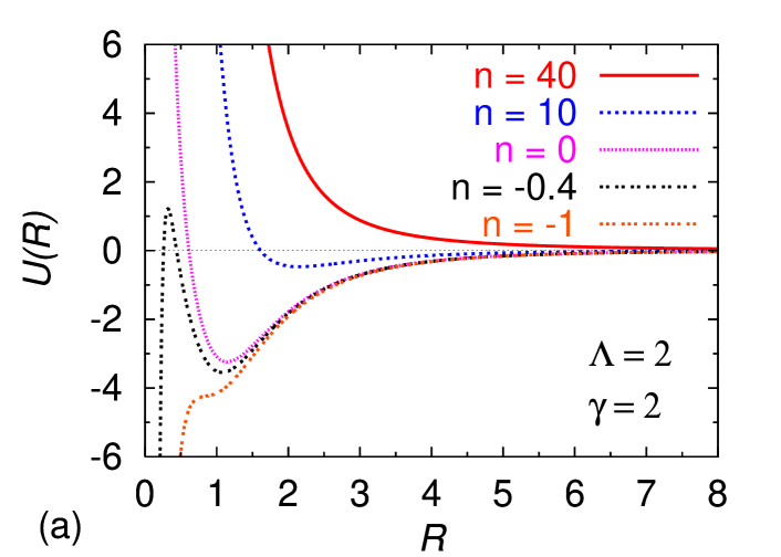
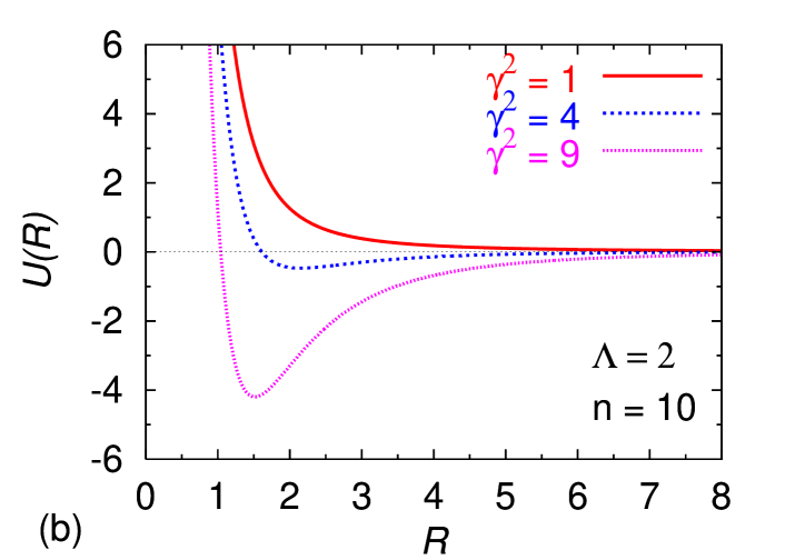
Figure 1: The effective potential $U(R)$ of Eq. (25) vs. $R$ in dimensionless units for $\Lambda=2$, (a) $\gamma=2$ and $n=40,10,0,-0.4,$ and -1 (upper to lower curves) and for (b) $n=10$ and $\gamma=1,2,$ and $3$ (upper to lower curves).

In Figs. 1 (a) and (b) we plot $U(R)$ vs $R$ of Eq. (25) in dimensionless units for different values of $n$, $\Lambda$ and $\gamma$. We exhibit $U(R)$ vs $R$ for different $n$ for $\Lambda=\gamma=2$ in Fig. 1 (a). The same for different $\gamma$ and $\Lambda=2$ and $n=10$ are exhibited in Fig. 1 (b). We find from Fig. 1 (a) that for a fixed $\gamma$ and $\Lambda$, $U(R)$ has a minimum for $n_{\mbox{lim}}>n>n_{\mbox{crit}}$ corresponding to a stable bound state, where $n_{\mbox{lim}}$ is positive (repulsive system) and $n_{\mbox{crit}}$ is negative (attractive system). In Fig. 1 (a) there is a minimum for $n=10,0$ and $-0.4$ and no minimum for $n=40$ and $-1$. The reason for the nonexistence of bound state for $n>n_{\mbox{lim}}$ and for $n<n_{\mbox{crit}}$ are distinct. The limiting condition $n>n_{\mbox{lim}}$ corresponds to a highly repulsive system which cannot be bound in the square-well potential with the given $\Lambda$ and $\gamma$. The condition $n<n_{\mbox{crit}}$ corresponds to a highly attractive system which collapses with the given $\Lambda$ and $\gamma$. In Fig. 1 (a) for $n=40$ the system is unbound and for $n=-1$ it is unstable to collapse. In Fig. 1 (a) we see that as the attractive nonlinearity $|n|$ is increased, one of the walls of the well for small $r$ is gradually lowered and for a sufficiently large attraction this wall is completely absent and the condensate collapses into the infinitely deep well at the center for $n=-1$ in Fig. 1 (a).

In Fig. 1 (b) we illustrate the effect of increasing the strength of the square-well potential for a fixed nonlinearity $n=10$. This is done by varying the depth of the square-well potential $\gamma^{2}$ for a fixed range $\Lambda$. For $\gamma=2$ and 3, $U(R)$ has a minimum and the attraction of the square-well potential is sufficient to bind the repulsive system with $n=10$. However, for $\gamma=1$ there is no minimum in $U(R)$ and the square-well potential is too weak to bind this system.

4 Numerical Result

We solve NLS equation (2) numerically for the square-well potential using the split-step time-iteration method employing the Crank-Nicholson discretization scheme described recently 11a ; 11b . We calculated the solutions with real-time propagation. However, we checked that imaginary-time propagation also leads to consistent result. To obtain the normalizable solution, the real time iteration is started with the known solution of the linear problem with scaled nonlinearity $n=0$. Then during time iteration the nonlinearity $n$ is switched on slowly until its desired value is attained. The change in the parameter should be such that it does not greatly alter the eigenvalue of the Hamiltonian (after time propagation). We also calculated the nonnormalizable bound states in the continuum for a positive $n$. To obtain this solution, the time iteration is started with a constant wave function for a finite positive $n$ with $\gamma=0$. Then in the course of time iteration the strength $\gamma$ of the square-well potential is switched on slowly until its desired value is attained. If stabilization upon time iteration could be achieved for the chosen parameters one already obtains the required nonlinear bound state in the square-well potential. In previous studies we compared critically the present numerical scheme for the time-dependent NLS equation with other approaches 11a ; 11b including the time-independent schemes adhi and assured that the present approach leads to results with high precision not only for the NLS equation with one space variable but also for NLS equations in two and three space variables am . The agreement between the results obtained with real and imaginary time propagation also assures the correctness of our results.

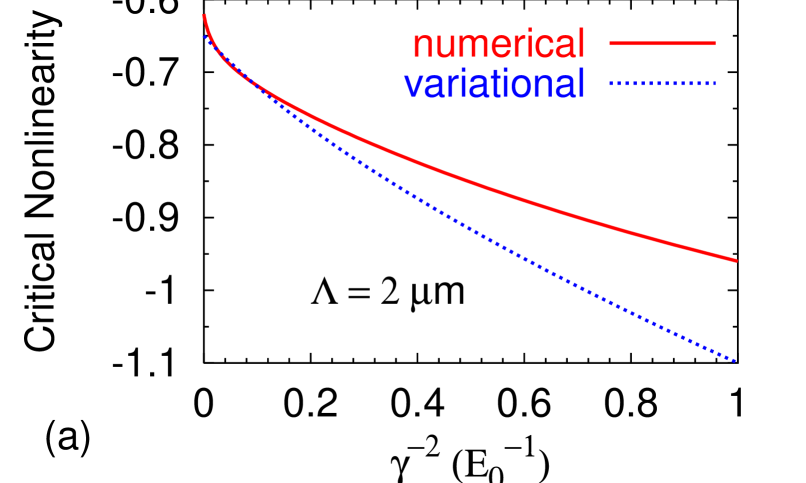
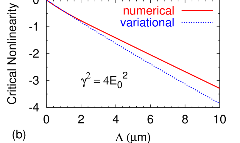
Figure 2: Critical nonlinearity $n_{\mbox{crit}}$ (a) vs. $\gamma^{-2}$ for $\Lambda=2$ $\mu$m and (b) vs. $\Lambda$ for $\gamma^{2}=4E_{0}\equiv 4\hbar\omega$: full line - numerical; dotted line - variational.

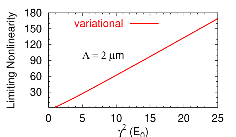
Figure 3: Limiting nonlinearity $n_{\mbox{lim}}$ vs. $\gamma^{2}$ for $\Lambda=2$ $\mu$m.

Although we calculate our results in dimensionless units, typical parameters for an experimental realization can be easily obtained therefrom for a particular atom. In the following we present results for the Rb atom. For Rb let the length $l$ be 1 $\mu$m; for this to be possible the reference frequency is $\omega\approx 2\pi\times 38$ Hz. Consequently, the unit of energy is $E_{0}\equiv\hbar\omega\approx 1.57\times 10^{-13}$ eV.

4.1 Normalizable States

Stable normalizable bound states are indeed found in all cases for various ranges of parameters. Some plausible properties of these bound state are found in agreement with the above variational study. For a given nonlinearity, these bound states are only formed for a sufficiently strong square-well potential determined by $\Lambda$ and $\gamma$. For weaker potentials, from the wisdom obtained in variational calculation, the effective potential $U(R)$ does not have a minimum and there cannot be any bound state. For a given square-well potential, bound states are found for $n_{\mbox{lim}}>n>n_{\mbox{crit}}$.

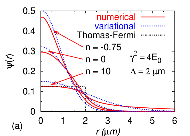
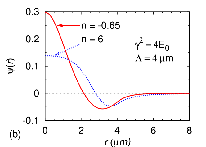
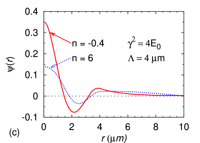
Figure 4: (a) Ground-state wave function $\psi(r)$ of the NLS equation (5) with the square-well potential for $\gamma^{2}=4E_{0}$, $\Lambda=2$ $\mu$m and scaled nonlinearity $n-0.75,0$ and 10 (upper to lower curves). In all cases the numerical and variational results are shown, in addition, for $n=10$ the TF approximation is also shown. (b) Same for the first excited soliton (numerical calculation only) with $\gamma^{2}=4E_{0}$, $\Lambda=4$ $\mu$m and $n=-0.65$ and 6. (c) Same for the second excited soliton (numerical calculation only) with $\gamma^{2}=4E_{0}$, $\Lambda=4$ $\mu$m and $n=-0.4$ and 6.

It is difficult to obtain the limiting nonlinearity $n=n_{\mbox{lim}}$ numerically as this corresponds to a state with zero energy which extends to a very large $r$. However, the critical value $n=n_{\mbox{crit}}$ can be obtained numerically in a controlled fashion as the wave function is highly localized in this limit. In Figs. 2 we plot the critical nonlinearity for collapse $n_{\mbox{crit}}$ for different parameters of the square-well potential. In Fig. 2 (a) we plot $n_{\mbox{crit}}$ vs. $\gamma^{-2}$ for $\Lambda=2$ $\mu$m whereas in Fig. 2 (b) we plot $n_{\mbox{crit}}$ vs. $\Lambda$ for $\gamma^{2}=4E_{0}$. In these figures we show results of variational and full numerical calculations. The variational calculation always leads to a larger $|n_{\mbox{crit}}|.$ In case of the infinite harmonic potential also, the variational estimate of $|n_{\mbox{crit}}|$ is larger than the result of full numerical calculation 8 . For the infinite square-well potential with $\gamma^{2}=\infty$ and $\Lambda=2$ $\mu$m, $n_{\mbox{crit}}=-0.62$; for the infinite parabolic potential $n_{\mbox{crit}}=-0.575$ 8 ; ad . Because of the different shapes of these two infinite potentials $n_{\mbox{crit}}$ is different in these two cases.

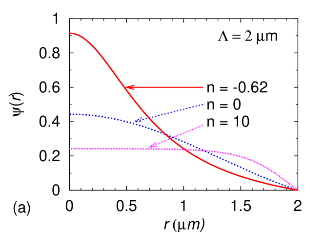
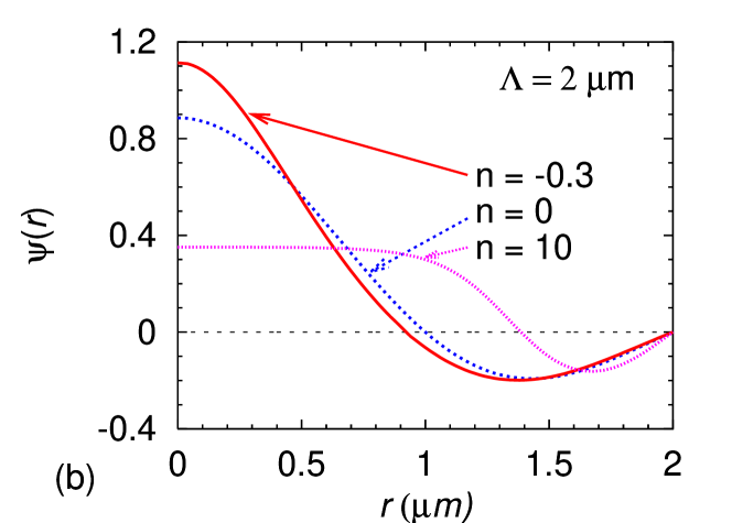
Figure 5: (a) Ground-state wave function $\psi(r)$ of the NLS equation (5) for the infinite square-well potential of range $\Lambda=2$ $\mu$m and scaled nonlinearity $n=-0.62,0$ and 10 (upper to lower curves); (b) same for the first excited soliton for $n=-0.3,0$ and 10.

Although it is difficult to obtain $n_{\mbox{lim}}$ from a numerical solution of the NLS equation, it is possible to obtain it from the variational calculation. The limiting nonlinearity $n_{\mbox{lim}}$ corresponds to the largest value of $n$ for which $U(R)$ has a minimum. In Fig. 3 we plot $n_{\mbox{lim}}$ vs. $\gamma^{2}$ for $\Lambda=2$ $\mu$m. We see that $n_{\mbox{lim}}$ increases linearly with the strength of the square well $\gamma^{2}$. The variational calculation underbinds the system. The repulsive nonlinearity destroys binding and a smaller repulsive nonlinearity can destroy the weaker binding of the variational model. Consequently, the variational limiting nonlinearity is smaller than the actual limiting nonlinearity, which we verified in our numerical calculation. The numerical calculation relies on the existence of a localized wave function and it is difficult to calculate the limit when this wave function extends to infinity and a localized wave function ceases to exist. The TF wave function (9) is always fully localized within $r<\Lambda$ and is inadequate for calculating the limiting nonlinearity for $\mu\to 0$. The TF wave function leads to a much smaller value $n_{\mbox{lim}}=\Lambda^{3}\gamma^{2}/6,$ based on imposing $\mu=0$ within the TF regime.

In Fig. 4 (a) we plot the wave function for the bound state of the NLS equation for a square-well potential with $\gamma^{2}=4E_{0}$, $\Lambda=2$ $\mu$m and for nonlinearities $n=-0.75,0$ and 10. The system with $n=-0.75$ is attractive, $n=0$ noninteracting, and $n=10$ repulsive. In these cases results for both the full numerical calculation and variational approximation are shown. In addition, for $n=10$ the TF approximation (10) with $c=\mu=0$ is also shown. In Fig. 4 (b) we show the wave functions for the first excited soliton with a single node for $\gamma^{2}=4E_{0}$ and $\Lambda=4$ $\mu$m and for $n=-0.65$ and 6. In Fig. 4 (c) we show the wave functions for the second excited soliton with two nodes for $\gamma^{2}=4E_{0}$ and $\Lambda=4$ $\mu$m and for $n=-0.4$ and 6. In Figs. 4 we find that the bound state for the attractive system with negative $n$ values is more centrally peaked than the bound state for the repulsive system with positive $n$ values. This is true for both ground and excited solitonic states in the finite square-well potential as well as for states in the infinite square-well potential studied below. The central peaking of the wave function for the attractive system corresponding to a large central probability density is a consequence of the nonlinear attraction.

Next we consider the infinite square-well potential of range $\Lambda$. In this case the system remains confined in the region $0\leq r\leq\Lambda$. The wave function is zero outside this region: $r>\Lambda$. We illustrate the wave functions in this case for different values of nonlinearity $n$ for the ground state and the first excited soliton for $\Lambda=2$ $\mu$m. For the ground state there is no node of the wave function for $0<r<\Lambda$. For the $j$th excited soliton these are $j$ nodes of the wave function in this region. The wave functions for the ground state and the first excited soliton for different $n$ are shown in Figs. 5 (a) and (b), respectively.

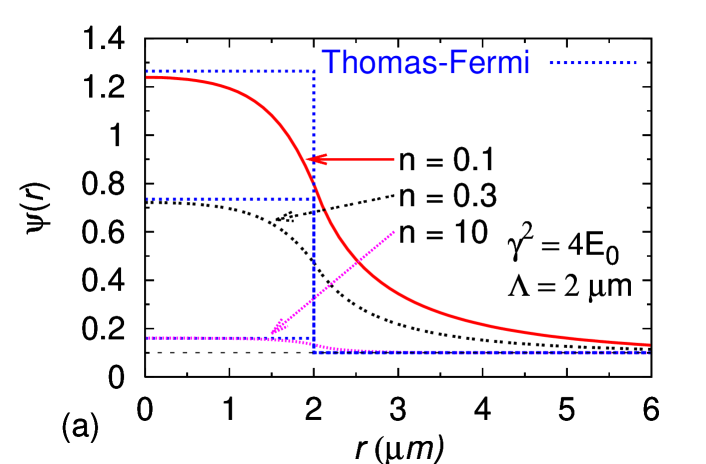
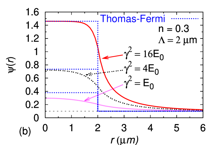
Figure 6: Wave functions of the nonnormalizable states $\psi(r)$ of the NLS equation (5) for (a) $\gamma^{2}=4E_{0}$, $\Lambda=2$ $\mu$m and different $n$ values, and for (b) $n=0.3$, $\Lambda=2$ $\mu$m and different $\gamma$. In both cases the wave function tends to $0.1$ as $r\to\infty.$ In all cases the results of the full numerical calculation and TF approximation are shown.

4.2 Nonnormalizable States

Now we discuss the nonnormalizable solutions of Eq. (2) obtained for repulsive condensates. No such states are found for attractive condensates with negative $n$. To obtain these solutions by time iteration of Eq. (2) we start with the initial constant solution $\psi(r)=0.1$ over all space for $V(r)=0$ and a fixed nonlinearity $n$. In the course of time iteration the square-well potential is slowly introduced without altering the nonlinearity until the full square-well potential is obtained. The resulting wave function of this calculation is plotted in Figs. 6 (a) and (b) together with the TF approximation. In Fig. 6 (a) we show the wave function for $\gamma^{2}=4E_{0}$, $\Lambda=2$ $\mu$m and $n=0.1,0.3,$ and 10. In Fig. 6 (b) we show the same for $\Lambda=2$ $\mu$m, $n=0.3$ and $\gamma^{2}=E_{0},4E_{0}$ and 16$E_{0}$. From Fig. 6 (a) we find that for a fixed $\gamma^{2}$ and $\Lambda$ the TF approximation becomes a better approximation as the nonlinearity increases; whereas from Fig. 6 (b) we find that for a fixed $\Lambda$ and $n$ the TF approximation becomes a better one as the strength of the potential $\gamma^{2}$ increases.

The normalizable states discussed in the last subsection are true bound states for negative $\mu$. The nonnormalizable states occur at positive $\mu$ and can be referred to as states in the continuum. Similar nonnormalizable states have been obtained in the study of the 1D NLS equation with the square-well potential c2 . However, there is the possibility of physically observing the nonnormalizable states with infinite norm as a transition from the normalizable states with very large nonlinearity c2 . An increase of the scattering length $a$ via a Feshbach resonance fesh in a BEC may increase the nonlinearity $n(\equiv Na/l)$ indefinitely and thus transform a normalizable state to a nonnormalizable one. This conclusion results from the following observation. As the normalization integral (4) and the nonlinearity $g=8\pi n$ of Eq. (2) are mixed in the present nonlinear model, an increase in $g$ can either be implemented my increasing the nonlinear term $g$ directly in Eq. (2) or by augmenting the normalization integral (4) in the same proportion. Hence the nonnormalizable states with very large (infinite) normalization could be a transition from normalizable states with large nonlinearity.

5 Discussion and Conclusion

The study of the 1D NLS equation with the simple square-well potential is of interest because of its simplicity and intrinsic nonlinear nature. Its interest in BEC and optics has motivated recent investigation of this problem c2 . In the 3D world, 1D systems can only be achieved in some approximation and there are nontrivial differences between the solutions of the NLS in 1D and 3D 1 .

Hence we performed in this paper an investigation of the 3D NLS equation with the square-well potential using numerical and variational solutions. We find that the system allows normalizable bound-state solutions for $n_{\mbox{lim}}>n>n_{\mbox{crit}}$, where the limiting nonlinearity $n_{\mbox{lim}}$ corresponds to a repulsive (positive) limit beyond which the system cannot be bound and the critical nonlinearity $n_{\mbox{crit}}$ to an attractive (negative) nonlinearity below which the system collapses. We calculated $n_{\mbox{crit}}$ for different parameters of the square-well potential. Many results of this paper can be verified experimentally in BEC, where one can make a square-well trap by joint magnetic and optical control c2 ; step2 . In addition to the discrete normalizable states we find that the 3D NLS equation with the square-well potential also sustains nonnormalizable states in the continuum of interest in nonlinear physics and mathematics. These states cannot be obtained via a transition from the normalizable states.

The work was supported in part by the CNPq and FAPESP of Brazil.

References

- (1) Y. S. Kivshar, G. P. Agrawal, Optical Solitons - From Fibers to Photonic Crystals, (Academic Press, San Diego, 2003.)
- (2) A. Hasegawa, F. Tappert, App. Phys. Lett. 23, 171 (1973); 23, 142 (1973).
- (3) V. E. Zakharov, A. B. Shabat, Sov. Phys. JETP 34, 62 (1972); 37, 823 (1973).
- (4) P. G. Kevrekidis, B. A. Malomed, D. J. Frantzeskakis, R. Carretero-González, Phys. Rev. Lett. 93, 080403 (2004); D. Mihalache, D. Mazilu, I. Towers, B. A. Malomed, F. Lederer, Phys. Rev. E 67, 056608 (2003); P. M. Lushnikov, M. Saffman, Phys. Rev. E 62, 5793 (2000); N. Aközbek, S. John, Phys. Rev. E 57, 2287 (1998); D. E. Edmundson, Phys. Rev. E 55, 7636 (1997); N. Akhmediev, J. M. Soto-Crespo, Phys. Rev. A 47, 1358 (1993).
- (5) F. Dalfovo, S. Giorgini, L. P. Pitaevskii, S. Stringari, Rev. Mod. Phys. 71, 463 (1999).
- (6) L. D. Carr, C. W. Clark, W. P. Reinhardt, Phys. Rev. A 62 063610 (2000); 62 063611 (2000).
- (7) L. D. Carr, K. W. Mahmud, W. P. Reinhardt, Phys. Rev. A 64 033603 (2001).
- (8) J. G. Muga, M. Buttiker, Phys. Rev. A 62, 023808 (2002); J. Villavicencio, R. Romo, S. S. Silva, Phys. Rev. A 66, 042110 (2002).
- (9) B. T. Seaman, L. D. Carr, M. J. Holland, Phys. Rev. A 71, 033609 (2005).
- (10) V. Hakim, Phys. Rev. E 55, 2835 (1997); D. Taras-Semchuk, J. M. F. Gunn, Phys. Rev. B 60, 013139 (1999).
- (11) Y. S. Kivshar, T. J. Alexander, S. K. Turitsyn, Phys. Lett. A 278, 225 (2001).
- (12) P. Leboeuf, N. Pavloff, S. Sinha, Phys. Rev. A 68, 063608, (2003); N. Pavloff, Phys. Rev. A 66, 013610, (2002).
- (13) M. Greiner, O. Mandel, T. Esslinger, T. W. Hänsch, I. Bloch, Nature (London) 415, 39 (2002).
- (14) L. D. Carr, M. J. Holland, B. A. Malomed, J. Phys. B 38, 3217 (2005).
- (15) S. K. Adhikari, Phys. Rev. A 69, 063613 (2004).
- (16) S. K. Adhikari, Phys. Rev. E 70, 036608 (2004); Phys. Rev. E 71, 016611 (2005).
- (17) L. I. Schiff, Quantum Mechanics, 3rd Ed. (McGraw-Hill, New York, 1968.)
- (18) F. K. Abdullaev, J. G. Caputo, R. A. Kraenkel, B. A. Malomed, Phys. Rev. A 67, 013605 (2003).
- (19) H. Goldstein, Classical Mechanics, 2nd Ed. (Addison Wesley, Reading, 1980).
- (20) S. K. Adhikari, P. Muruganandam, J. Phys. B 35, 2831 (2002).
- (21) P. Muruganandam, S. K. Adhikari, J. Phys. B 36, 2501 (2003).
- (22) S. K. Adhikari, Phys. Lett. A 265, 91 (2000); Phys. Rev. E 62, 2937 (2000); Phys. Rev. C 19, 1729 (1979); S. K. Adhikari and A. Ghosh, J. Phys. A 30, 6553 (1997).
- (23) S. K. Adhikari, P. Muruganandam, Phys. Lett. A 310, 229 (2003).
- (24) S. K. Adhikari, Phys. Rev. E 65, 016703 (2002).
- (25) S. Inouye, M. R. Andrews, J. Stenger, H. J. Miesner, D. M. Stamper-Kurn, W. Ketterle, Nature 392, 151 (1998).