Understanding Kondo Peak Splitting and the Mechanism of Coherent Transport in a Single-Electron Transistor

Abstract

The peculiar behavior of Kondo peak splitting under a magnetic field and bias can be explained by calculating the nonequilibrium retarded Green’s function via the nonperturbative dynamical theory (NDT). In the NDT, the application of a lead-dot-lead system reveals that new resonant tunneling levels are activated near the Fermi level and the conventional Kondo peak at the Fermi level diminishes when a bias is applied. Magnetic field causes asymmetry in the spectral density and transforms the new resonant peak into a major peak whose behavior explains all the features of the nonequilibrium Kondo phenomenon. We also show the mechanism of coherent transport through the new resonant tunneling level.

After the observation of the equilibrium Kondo phenomenon in a single-electron transistor (SET)1 , nonequilibrium Kondo phenomenon has rapidly evolved into one of the highly debated subjects in condensed matter physics. As the phenomenon entails two theoretically challenging field of study, namely nonequilibrium and strong correlation, thus far no theoretical study has been successfully able to explain the experiments exhibiting the nonequilibrium Kondo phenomenon fully2 ; 3 . Therefore, a theoretical understanding of this phenomenon would be an essential development in the advancement of condensed matter physics. The most attractive aspect of the nonequilibrium Kondo phenomenon is the splitting of the Kondo peak under a magnetic field2 ; 3 . According to the experiment performed by Amasha et al.3 , nonequilibrium Kondo phenomena can be summarized as follows: (i) splitting vs. magnetic field, which is expressed by a simple relation $\Delta_{{\rm K},S}=\Delta_{{\rm K},S}^{0}+|g|\mu_{B}B$, where $\Delta_{{\rm K},S}$ denotes half of the gap between the split Kondo peaks, the superscript $0$ denotes field-independence, and the subscript $S$ denotes particle-hole symmetric case; (ii) splitting vs. gate voltage, which is given by $\Delta_{\rm K}^{0}=\Delta_{{\rm K},S}^{0}-C_{0}(V_{\rm g}-V_{{\rm g},0})^{2}$, where $V_{{\rm g},0}$ denotes the gate voltage in the middle of the Coulomb valley and the curvature of the parabola $C_{0}$ is field-independent; (iii) splitting vs. Kondo temperature, which appears to be logarithmically decreasing, i.e., $\Delta_{\rm K}^{0}(T_{\rm K})\propto-C_{1}\ln T_{\rm K}$, where $C_{1}$ is also field-independent; and (iv) the maximum Kondo temperature $T_{\rm Km}$ vs. the critical magnetic field $B_{\rm C}$ at the splitting threshold, which is nonlinear. One notable issue common to all the abovementioned features is the field-independent behaviors of $\Delta_{{\rm K},S}^{0}$, $C_{0}$, and $C_{1}$. Existing theories4 cannot explain the field-independent behaviors in (i), (ii), and (iii) and the nonlinear behavior in (iv). We will show that these can be explained by the nonperturbative dynamical theory (NDT)5 .

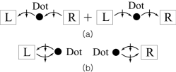
Figure 1: Motions of spin-down electron in the first (a) and second (b) type of coherence. In (b), left one corresponds to $Z^{LL}$ while right one to $Z^{RR}$.

Figure 2: The spectral density of the SET for $U=10\Delta$ under a bias, where $\Delta=\Gamma/2$. The Zeeman shift is $0.5\Delta$. The inset is for that under equilibrium.

The result of NDT shows that the Kondo peak in equilibrium comprises two different types of coherence whose spectral weights will be denoted by $Z_{S}^{LR}$ and $Z_{S}^{LL}$ below. In the first type of coherence, the spin-down electron, for instance, travels back and forth through the dot as shown in Fig. 1 (a), while it moves as that shown in Fig. 1 (b) in the second type of coherence. The spin-up electron arrives toward the dot from the left or right lead in both the cases. The spectral density has a single resonant peak in equilibrium as shown in the inset of Fig. 2. Because of two separate metallic reservoirs, the maximum of $\pi\Delta\rho_{d\uparrow}(\omega)$ is $0.5$ instead of unity.

The most interesting result of NDT appears when a bias is applied. A part of the spectral weight of $Z_{S}^{LR}$ transfers from the Fermi level to the new resonant tunneling levels near the Fermi level, while the spectral weight $Z_{S}^{LL}$, which corresponds to the second type of coherence, remains at the Fermi level. However, the weight $Z_{S}^{LL}$ at the Fermi level is suppressed by decoherence due to bias. Interesting point is that the position of the new resonant level is independent of the applied field. This field-independence is responsible for the field independent features of the Kondo-peak splitting mentioned above.

When magnetic field is applied, an asymmetry occurs in the spectral density in addition to the usual Zeeman shift $|g|\mu_{B}B$. As a result of asymmetry, one of the new resonant peaks becomes a major peak as shown in Fig. 2. All the abovementioned features of the Kondo peak splitting phenomenon can be explained by the position of this major peak. In order to draw the spectral density $\rho_{d\uparrow}(\omega)$, we artificially choose the parameters of the spectral density to show the asymmetry and the suppression of the central peak explicitly. The correct values of the parameters may be determined by the self-consistent calculation proposed in Ref. [5].

The result of NDT gives the positions of the new resonant peak as $\pm\sqrt{Z_{S}^{LL}}U/2$ in the Kondo regime with particle-hole symmetry, where $U$ is the amount of Coulomb repulsion at the dot. Therefore, the field-independent splitting in feature (i) mentioned earlier is given by $\Delta_{{\rm K},S}^{0}=\sqrt{Z_{S}^{LL}}U/2$. Since asymmetry is involved in the part that becomes $U$ in the symmetric case, we propose the following expression of $\Delta_{\rm K}^{0}$ for the asymmetric case:

$$\Delta_{\rm K}^{0}=\sqrt{Z_{S}^{LL}}\left[\frac{4\sqrt{2}\Gamma}{\pi}\ln\frac{\widetilde{D}}{Z\Gamma}\right],$$ (1)

where $Z=Z^{LL}+Z^{LR}$ and $\widetilde{D}=Z_{S}\Gamma\,{\rm exp}[\pi U/8\sqrt{2}\Gamma]$. Equation (1) recovers $\Delta_{{\rm K},S}^{0}$ if $Z=Z_{S}$. If we use the notations given in Ref. [3], the wavefunction renormalization $Z$ can be rewritten as $Z=Z_{S}{\rm exp}[\chi(V_{\rm g}-V_{{\rm g},0})^{2}]=Z_{S}T_{\rm K}/T_{\rm K,0}$, where $V_{\rm g}$ denotes the gate voltage and $T_{\rm K,0}$ is the Kondo temperature at gate voltage in the middle of the Coulomb valley $V_{{\rm g},0}$. Then, the asymmetric behavior of $\Delta_{\rm K}^{0}$ is given by the parabolic or logarithmic form

$$\Delta_{\rm K}^{0} = \Delta_{{\rm K},S}^{0}-\frac{8\sqrt{2}\Gamma}{\pi U}\Delta_{{\rm K},S}^{0}\,\chi(V_{\rm g}-V_{{\rm g},0})^{2}$$

$$= \Delta_{{\rm K},S}^{0}-\frac{8\sqrt{2}\Gamma}{\pi U}\Delta_{{\rm K},S}^{0}\ln(T_{\rm K}/T_{\rm K,0}).$$

These expressions simultaneously explain all the abovementioned features of the Kondo peak splitting in a qualitative manner, except for the feature of the splitting threshold. The curvature of the parabola and the coefficient in the $-\ln T_{\rm K}$-dependence are given by $C_{0}=-8\sqrt{2}\Gamma\Delta_{{\rm K},S}^{0}\chi/\pi U$ and $C_{1}=8\sqrt{2}\Gamma\Delta_{{\rm K},S}^{0}/\pi U$, respectively. Since the values of the constants $C_{0}$ and $C_{1}$ are given by $C_{0}=-0.22\mu$eV/(mV)² and $C_{1}=11\mu$eV, respectively, using the experimental values $\Gamma=330\mu$eV, $U=1.2$meV, $\chi=0.020$(mV)^-2, and $\Delta_{\rm K,S}^{0}=11\mu{\rm eV}$, quantitative agreement with the experimental data is perfect.

Figure 3: Relationship between $T_{\rm Km}$ and $B_{\rm C}$ at the splitting threshold.

The threshold of the Kondo peak splitting depends on both the width of the peak and the positions of the major peaks produced by both the spin-up and spin-down electrons. Since the width of Kondo peak is linearly proportional to the Kondo temperature, the linear deviation of the Kondo temperature from its minimum, i.e., $T_{\rm K}-T_{\rm K,0}$ will play an important role in constructing the threshold equation. We now consider relative positions of the major peaks. For the field $|g|\mu_{B}B=\Delta_{\rm K}^{0}$, the major peak of $\rho_{d\uparrow}(\omega)$ appears at $2\Delta_{\rm K}^{0}$ above the Fermi level, while that of $\rho_{d\downarrow}(\omega)$ is located at the Fermi level. In this case, no separation will be observed because the major peak of $\rho_{d\downarrow}(\omega)$ for a reversed bias has the same position with that of the forward bias. The spectral densities for forward and reverse bias are mirror-reflected with respect to the vertical axis.

We assume that the separation may be clearly observed when the major peak of $\rho_{d\downarrow}(\omega)$ appears at a position lower than $\Delta_{\rm K}^{0}$ below the Fermi level, i.e., $|g|\mu_{B}B+\Delta^{0}_{\rm K}(T_{\rm K})\geq 3\Delta^{0}_{\rm K}(T_{{\rm K},0})$. If we combine this with the effect of Kondo temperature mentioned above, we write the threshold equation as $|g|\mu_{B}B_{\rm C}+\Delta^{0}_{\rm K}(T_{\rm Km})=3\Delta^{0}_{{\rm K},S}[1+(T_{\rm Km}-T_{\rm K,0})/4T_{\rm K,0}]$, where $\Delta^{0}_{{\rm K},S}=\Delta^{0}_{\rm K}(T_{{\rm K},0})$ and $T_{\rm Km}$ is the maximum Kondo temperature at threshold. At $T_{\rm K}=T_{\rm K,0}$, $B_{\rm C}=2\Delta_{{\rm K},S}^{0}/|g|\mu_{B}$, which corresponds to $B_{\rm C}=2.4{\rm T}$ for $\Delta_{{\rm K},S}^{0}=11\mu{\rm eV}$ and $|g|=0.16$3 . The coefficient $3\Delta^{0}_{{\rm K},S}/4T_{\rm K,0}$ has been introduced phenomenologically. Remarkable agreement with the experiment is shown in Fig. 3, if we use the experimental value $T_{\rm K,0}=0.25$K3 .

We successfully explained the experiments using Eq. (1). Now, it is right time to derive Eq. (1) by calculating the retarded Green’s function $G_{dd\uparrow}^{+}(\omega)$ under nonequilibrium conditions. We use the NDT that provides a new technique to calculate $G_{dd\uparrow}^{+}(\omega)$5 , which is expressed as $G_{dd\sigma}^{+}(\omega)=\langle c_{d\sigma}|(\omega+i\eta-{\rm\bf L})^{-1}|c_{d\sigma}\rangle$ in the Heisenberg picture6 , where ${\rm\bf L}$ is the Liouville operator defined by ${\rm\bf L}{A}={H}{A}-{A}{H}$ where $H$ is the Hamiltonian, $\eta$ is a positive infinitesimal, and the inner product is defined as $\langle A|B\rangle\equiv\langle\{{A},{B}^{\dagger}\}\rangle$, where ${A}$ and ${B}$ are the operators of the Liouville space, the curly brackets denote the anticommutator, and the last angular brackets represent a nonequilibrium average5 . If we define the elements of the matrix ${\rm\bf M}$ as ${\rm\bf M}_{ij}=\langle{\hat{e}}_{j}|z{\rm\bf I}+i{\rm\bf L}|{\hat{e}}_{i}\rangle$, where $z=-i\omega+\eta$ and the operator ${\hat{e}}_{j}$ is one of the bases spanning the Liouville space, the retarded Green’s function is represented by $iG_{dd\sigma}^{+}(\omega)=\langle c_{d\sigma}|{\rm\bf M}^{-1}|c_{d\sigma}\rangle=({\rm adj}\,\,{\rm\bf M})_{dd}[{\rm det}\,\,{\rm\bf M}]^{-1}$, where $({\rm adj}\,\,{\rm\bf M})_{ij}$ denotes the cofactor of the $ji$-element in the determinant of ${\rm\bf M}$.

The NDT is initiated by constructing a complete set of dynamical bases $\{{\hat{e}}_{j}|j=1,2,\cdots,\infty\}$ spanning the reduced Liouville space in which the dynamics of the operator $c_{d\sigma}(t)$ effectively describes the Kondo processes. We simply extend the bases for the single-impurity Anderson model used in the previous study5 to the case of two metallic reservoirs described by the Hamiltonian $H=\sum_{k,\sigma,\alpha=L,R}\epsilon_{k}c^{\alpha\dagger}_{k\sigma}c^{\alpha}_{k\sigma}+\sum_{k,\sigma,\alpha=L,R}(V_{kd}c^{\dagger}_{d\sigma}c^{\alpha}_{k\sigma}+V^{*}_{kd}c^{\alpha\dagger}_{k\sigma}c_{d\sigma})+\sum_{\sigma=\pm 1}(\epsilon_{d}-\sigma g|\mu_{B}|B)c^{\dagger}_{d\sigma}c_{d\sigma}+Un_{d\uparrow}n_{d\downarrow},$ in which $L$ and $R$ denote the left and right leads, respectively, and the subscript $k$ denotes the quantum state of the metallic leads and $n_{d\downarrow}=c_{d\downarrow}^{\dagger}c_{d\downarrow}$. Then, the basis operators comprise the following five sets: (a) $S^{L}_{k}\equiv\{c^{L}_{k\uparrow}|k=1,2,\cdots,\infty\}$ for describing the movements in the left noninteracting metallic lead, (b) $S^{L}_{n}\equiv\{\delta n_{d\downarrow}c^{L}_{k\uparrow}|k=1,2,\cdots,\infty\}$ for describing the annihilation of a spin-up electron in the left lead combined with the density fluctuations in the spin-down electron at the dot, (c) and (d) the sets similar to (a) and (b) for the right lead, i.e., $S^{R}_{k}$ and $S^{R}_{n}$, respectively, and (e) $S_{d}\equiv\{\delta j^{-L}_{d\downarrow}c_{d\uparrow},\delta j^{+L}_{d\downarrow}c_{d\uparrow},c_{d\uparrow},\delta j^{+R}_{d\downarrow}c_{d\uparrow},j^{-R}_{d\downarrow}c_{d\uparrow}\}$ for describing the dynamical Kondo processes at the dot.

If we symmetrically arrange the bases such as $S_{k}^{L}$, $S_{n}^{L}$, $S_{d}$, $S_{n}^{R}$, and $S_{k}^{R}$ to construct the matrix ${\rm\bf M}$, the following matrix of nine blocks is obtained:

$${\rm\bf M}_{\ell d\ell}=\left(\begin{array}[]{ccc}{\rm\bf M}_{LL}\,\,\,\,\,{\rm\bf M}_{dL}\,\,\,\,\,\,{\rm\bf 0}\\ {\rm\bf M}_{Ld}\,\,\,\,\,\,{\rm\bf M}_{d}\,\,\,\,\,\,\,{\rm\bf M}_{Rd}\\ \,\,\,\,{\rm\bf 0}\,\,\,\,\,\,\,\,\,\,\,\,{\rm\bf M}_{dR}\,\,\,\,{\rm\bf M}_{RR}\end{array}\right),$$

where the blocks ${\rm\bf M}_{d}$, ${\rm\bf M}_{dL}$ and ${\rm\bf M}_{dR}$, and ${\rm\bf M}_{Ld}$ and ${\rm\bf M}_{Rd}$ are $5\times 5$, $5\times\infty$, and $\infty\times 5$ matrices, respectively. Blocks ${\rm\bf M}_{LL}$ and ${\rm\bf M}_{RR}$ are the $\infty\times\infty$ matrices that are constructed by the sets of bases describing the left and right leads, respectively. Since no direct coupling exists between the left and right leads, zero matrices occur at the two corners. The structure of each block is similar to that of the corresponding block of the matrix for the Anderson model considered in the previous study5 .

The infinite-dimensional matrix can be reduced to a finite-dimensional matrix using the Löwdin’s partitioning technique7 ; 8 . It is performed by solving the eigenvalue equation for the matrix ${\rm\bf M}_{\ell d\ell}$, such as ${\rm\bf M}_{\ell d\ell}{\rm\bf C}={\rm\bf 0}$, where ${\rm\bf C}$ and ${\rm\bf 0}$ are the infinite-dimensional column vectors. The column vector ${\rm\bf C}$ is partitioned into three parts, i.e., ${\rm\bf C}^{T}=({\rm\bf C}^{L}\,{\rm\bf C}^{d}\,{\rm\bf C}^{R})$, where $T$, $L$, $d$, and $R$ denote the transpose, left lead, dot, and right lead, respectively. Then, the equation for ${\rm\bf C}^{d}$ is obtained as $({\rm\bf M}_{d}-{\rm\bf M}_{Ld}{\rm\bf M}_{LL}^{-1}{\rm\bf M}_{dL}-{\rm\bf M}_{Rd}{\rm\bf M}_{RR}^{-1}{\rm\bf M}_{dR}){\rm\bf C}^{d}\equiv{\widetilde{\rm\bf M}}_{d}{\rm\bf C}^{d}={\rm\bf 0}$. The reduced $5\times 5$ matrix ${\widetilde{\rm\bf M}}_{d}$ contains information on the many-body dynamics of the spin-up electron. Obtaining ${\widetilde{\rm\bf M}}_{d}$ is practically possible if the $\infty\times\infty$ matrices ${\rm\bf M}_{LL}$ and ${\rm\bf M}_{RR}$ are block diagonal9 . The second and third terms appear as self-energies in ${\widetilde{\rm\bf M}}_{d}$ after reduction.

The matrix ${\widetilde{\rm\bf M}}_{d}$ is expressed as

$$\widetilde{\rm\bf M}_{d}=\left(\begin{array}[]{ccccc}-i\tilde{\omega}\,\,\,\,\,\,\,-\gamma_{LL}\,\,\,\,\,\,\,\,-U^{L}_{J^{-}}\,\,\,\,\,\,\,\,\gamma_{LR}\,\,\,\,\,\,\,\,\gamma_{J^{-}}\\ \\ \,\,\gamma_{LL}\,\,\,\,\,\,\,\,-i\tilde{\omega}\,\,\,\,\,\,-U^{L}_{J^{+}}\,\,\,\,\,\,\,\,\,\,\gamma_{J^{+}}\,\,\,\,\,\,\,\gamma_{LR}\\ \\ \,\,\,\,\,\,U_{J^{-}}^{L*}\,\,\,\,\,\,\,\,\,\,U_{J^{+}}^{L*}\,\,\,\,\,\,\,-i\tilde{\omega}\,\,\,\,\,\,\,\,\,\,\,U^{R*}_{J^{+}}\,\,\,\,\,\,\,\,\,\,U^{R*}_{J^{-}}\\ \\ \,\,-\gamma_{LR}\,\,\,\,\,\,\,\,-\gamma_{J^{+}}\,\,\,\,\,\,\,\,-U_{J^{+}}^{R}\,\,\,\,-i\tilde{\omega}\,\,\,\,\,\,\,\,\,\,\gamma_{RR}\\ \\ \,\,\,\,-\gamma_{J^{-}}\,\,\,\,\,\,-\gamma_{LR}\,\,\,\,\,-U_{J^{-}}^{R}\,\,-\gamma_{RR}\,\,\,-i\tilde{\omega}\end{array}\right),$$

where $\tilde{\omega}\equiv\omega-\epsilon_{d}-U\langle n_{d\downarrow}\rangle+g|\mu_{B}|B$. All the matrix elements, other than $U_{J^{\pm}}$ and $U_{J^{\pm}}^{*}$, have additional self-energy functions $i\Sigma_{ij}(\omega)=\beta_{ij}(i\Sigma^{L}_{0}(\omega)+i\Sigma^{R}_{0}(\omega))$, where $\Sigma_{0}(\omega)$ is the self-energy for the Anderson model at $U=0$10 . The coefficient $\beta_{33}=1$ and others, $\beta_{ij}=\beta_{ji}$, are given by $\beta_{22}=\beta_{24}=\beta_{44}>\beta_{12}=\beta_{14}>\beta_{11}=\beta_{55}>\beta_{15}>\beta_{25}=\beta_{45}$11 . In equilibrium at half-filling, however, $\beta_{ij}=1/4$ except $\beta_{33}$. We use that $\gamma_{LL}=\gamma_{RR}$ and $\gamma_{J^{-}}=\gamma_{J^{+}}$. The latter will be discussed below.

In particular, it is noteworthy that the zeros of the determinant of $\widetilde{\rm\bf M}_{d}$ are $\tilde{\omega}=0,\pm[\gamma_{LL}^{2}+(\gamma_{LR}-\gamma_{J^{\pm}})^{2}]^{1/2}$, and $\pm U/2$ in the large-$U$ and atomic limit. The second zeros become $\pm\gamma_{LL}$ under appropriate amount of bias. This implies that there are additional resonant tunneling levels at $\pm\gamma_{LL}$ if we treat the system with two separate leads. One of the effects of the magnetic field is the Zeeman shift appearing in $\tilde{\omega}$ in the diagonal elements. We use $\omega$ to represent $\omega-\epsilon_{d}-U\langle n_{d\downarrow}\rangle$ hereafter. The Zeeman shift results in a nonvanishing value of $1/2-\langle n_{d\downarrow}\rangle$ that induces asymmetry in the spectral density by the nonvanishing imaginary part of the elements $U_{J^{\pm}}$, which can be expressed as $U_{J^{\pm}}=(U/4)[1+i2(1-2\langle n_{d\downarrow}\rangle)\langle j^{\pm}_{d\downarrow}\rangle/\langle(\delta j^{\pm}_{d\downarrow})^{2}\rangle^{1/2}]$. The asymmetry maximizes the new resonant peak appearing at $\omega=g\mu_{B}B+\gamma_{LL}$, as shown in Fig. 2. Therefore, the field-independent part of the splitting $\Delta^{0}_{{\rm K},S}$ is merely $\gamma_{LL}$. The real part of $U_{J^{\pm}}$ determines the positions of the $U$-peaks. The coefficient $1/4$ was determined from the analysis performed at the atomic limit. It is $1/\sqrt{2}$ times smaller than that of the single impurity Anderson model5 .

Since $\gamma_{LL}=\langle\sum_{k}i(V_{kd}^{*L}c_{k\uparrow}^{L}+V_{kd}^{*R}c_{k\uparrow}^{R})c^{\dagger}_{d\uparrow}[j^{-L}_{d\downarrow},j^{+L}_{d\downarrow}]\rangle$, its direct calculation is difficult12 . We have tried direct calculation of $\gamma_{LL}$ in our previous work13 . We have obtained that $\gamma_{LL}\propto\ln(\widetilde{D}/Z\Gamma)$. However, we failed to derive a correct prefactor of $\ln(\widetilde{D}/Z\Gamma)$ in the previous work, which is necessary to explain the experimental results quantitatively. Even though the NDT provides us all qualitative features of the Kondo peak splitting phenomenon, we need correct prefactor of $\ln(\widetilde{D}/Z\Gamma)$ for the quantitative comparison with experiment. An indirect way employing the exact result by Bethe Ansatz10 make it possible to derive an appropriate expression of $\gamma_{LL}$.

The wavefunction renormalization $Z$ can also be obtained by calculating the spectral weight of $\rho_{d\uparrow}(\omega)$ at $\omega=0$. Under equilibrium with particle-hole symmetry, it is given by $Z_{S}=[1+U^{2}/\{4(\gamma_{LL}^{2}+\gamma_{LR}^{2})\}]^{-1}$, where $\gamma_{LR}=\langle\sum_{k}i(V_{kd}^{*L}c_{k\uparrow}^{L}+V_{kd}^{*R}c_{k\uparrow}^{R})c^{\dagger}_{d\uparrow}[j^{-L}_{d\downarrow},j^{+R}_{d\downarrow}]\rangle$. In the Kondo regime, $Z_{S}$ gets separated into two parts, i.e., $Z^{LL}_{S}=4\gamma_{LL}^{2}/U^{2}$ and $Z^{LR}_{S}=4\gamma_{LR}^{2}/U^{2}$. The former is the spectral weight remaining at the Fermi level, which does not contribute to the Kondo peak splitting, and the latter, which is responsible for the Kondo peak splitting, transfers to the new resonant tunneling level at $\omega=\gamma_{LL}$ and gives rise to the additional shift $\sqrt{Z_{S}^{LL}}U/2$ to the one by Zeeman effect.

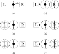
Figure 4: Coherent transport through the new resonant tunneling level when a spin-up electron hops into the dot.

As one can see from the operator expression of $\gamma_{LL}$, it is independent of the Coulomb repulsion. Therefore, $U$ appearing in the expression of $\gamma_{LL}$ should come from the averaging process and may be expressed by $Z$. The theory using Bethe ansatz yields $Z_{S}=(4/\pi)\sqrt{U/\Gamma}{\rm exp}[-\pi U/4\Gamma]$ for the symmetric Anderson model in the Kondo regime10 . Then, $U$ is written as $U=(4\Gamma/\pi)\ln(\widetilde{D}/Z_{S}\Gamma)$, where $\widetilde{D}=Z_{S}\Gamma{\rm exp}[\pi U/4\Gamma]$. For the Anderson model with two separate reservoirs, however, the effect of the two reservoirs changes $U$ and $\Gamma$ into $U/\sqrt{2}$ and $2\Gamma$, respectively. Therefore, $Z_{S}=(4/\pi)\sqrt{U/2\sqrt{2}\Gamma}{\rm exp}[-\pi U/8\sqrt{2}\Gamma]$ for the SET in the Kondo regime. By using the expression for $U$ from the $Z_{S}$ for the SET and removing the subscript $S$ to take the asymmetry into account, we obtain $\gamma_{LL}=(4\sqrt{2}\Gamma/\pi)\sqrt{Z_{S}^{LL}}\ln(\widetilde{D}/Z\Gamma)$, where $\widetilde{D}=Z_{S}\Gamma{\rm exp}[\pi U/8\sqrt{2}\Gamma]$. This is just Eq. (1).

It is interesting and meaningful to observe the mechanism of electron transport through the new resonant tunneling level in an SET. This mechanism appears in the operator expressions of $\gamma_{LR}$. The motion of the spin-down electron is governed by the operator $[j^{-L}_{d\downarrow},j^{+R}_{d\downarrow}]$, as described in Fig. 1 (a), while spin-up electron moves into the dot from the left or the right lead. Figure 4 shows the process making current when the chemical potential of the right lead is higher than that of left. Since the movement that costs energy $U$ is not allowed, a possible operation that constitutes a current is the one in which a spin-up electron moves from the right lead to the dot, makes a singlet coupling with a spin-down electron on the right lead, and moves together toward the left lead. Then, the spin-down electron changes its partner that is a spin-up electron on the right lead to make a singlet. This new singlet moves to the left and the process is repeated. It is noteworthy that the singlet state is retained during transport and the partner of singlet is changed, similar to that in superconductivity.

The motion of the spin-down electron of the operator $[j^{\mp L}_{d\downarrow},j^{\mp R}_{d\downarrow}]$ in $\gamma_{J^{\mp}}=\langle\sum_{k}i(V_{kd}^{*L}c_{k\uparrow}^{L}+V_{kd}^{*R}c_{k\uparrow}^{R})c^{\dagger}_{d\uparrow}[j^{\mp L}_{d\downarrow},j^{\mp R}_{d\downarrow}]\rangle$ is Fig. 1 (a) with $-$ sign, which corresponds to the net flow of the spin-down electrons. When the bias increases, $\gamma_{J^{\mp}}$ approaches $\gamma_{LR}$ and the spectral weight of the new resonant peak also increases. However, at equilibrium, $\gamma_{J^{\mp}}$ vanishes and the new resonant peak disappears.

In conclusion, we report the existence of a new resonant tunneling level in an SET with a strong correlation. This new resonant tunneling level is activated only under nonequilibrium conditions, and it explains all the features of the Kondo peak splitting phenomenon measured by Amasha et al.3 . Further, we show in Fig. 4 the coherent transport mechanism through the dot using the new resonant tunneling level.

This work was supported by the Korea Research Foundation, Grant No. KRF-2006-0409-0060.

References

(1) D. Goldhaber-Gordon et al., Nature (London)
391, 156 (1998); D. Goldhaber-Gordon et al., Phys.
Rev. Lett. 81, 5225 (1998).
(2) A. Kogan et al., Phys. Rev. Lett. 93,
166602 (2004).
(3) S. Amasha, I. J. Gelfand, M. A. Kastner, and A. Kogan, Phys. Rev. B 72,
045308 (2005).
(4) J. E. Moore and X.-G. Wen, Phys. Rev. Lett. 85,
1722 (2000); T. A. Costi, Phys. Rev. Lett. 85, 1504 (2000).
(5) J. Hong and W. Woo, cond-mat/0701765v3.
(6) P. Fulde, Electronic Correlations in Molecules
and Solids (Springer-Verlag, Berlin, 1993).
(7) P. O. Löwdin, J. Math. Phys. 3, 969
(1962).
(8) V. Mujica, M. Kemp, and M. A. Ratner, J. Chem. Phys.
101, 6849 (1994).
(9) A. S. Householder, Principles of Numerical
Analysis (McGraw-Hill, New York, 1953), pp. 78.
(10) A. C. Hewson, The Kondo Problem to Heavy
Fermions (Cambridge University Press, Cambridge, UK, 1993).
(11) The expression , for instance, is given by
, where
,
, and
.
(12) We omit the normalization factor in the expressions of all ’s.
(13) J. Hong and W. Woo, J. Kor. Phys. Soc. 49, 2230
(2006).