Detection of finite frequency current moments with a dissipative resonant circuit

Abstract

We consider the measurement of higher current moments with a dissipative resonant circuit, which is coupled inductively to a mesoscopic device in the coherent regime. Information about the higher current moments is coded in the histograms of the charge on the capacitor plates of the resonant circuit. Dissipation is included via the Caldeira-Leggett model, and it is essential to include it in order for the charge fluctuations (or the measured noise) to remain finite. We identify which combination of current correlators enter the measurement of the third moment. The latter remains stable for zero damping. Results are illustrated briefly for a quantum point contact.

The knowledge of all current moments, at arbitrary frequencies, allows to characterize completely the statistics of electron transfer in mesoscopic devices. The lowest current moments have recently been measured experimentally for a few specific systems reulet ; reznikov ; fujisawa . Zero frequency noise measurements have provided valuable diagnosis for transport in the past, yet current moments at high frequencies are difficult to measure, and typically require an on-chip measuring apparatusaguado_kouwenhoven ; deblock_science ; onac ; lesovik_loosen . Finite frequency noise contains information which is not apparent at zero frequency, when characterizing excitations in carbon nanotubes trauzettel_lebedev . Here, we present a scheme for the measurement of the noise and third moment at high frequencies, using a resonant circuit. A central issue deals with the electromagnetic environment on such measurements, which has been discussed in the past in different contexts beenaker ; other .

On-chip noise measuring proposals are either based on capacitive coupling, on inductive coupling, or bothgabelli . Any measurement involves the filtering of frequencies by the detection circuit, with an appropriate bandwidth: this justifies the choice of a generic resonant circuit. A dissipationless LC circuit was proposedlesovik_loosen to measure high frequency noise. The measured noise (the squared charge fluctuations on the capacitor) is then a combination of the unsymmetrized current correlators. The charge fluctuations are inversely proportional to the adiabatic switching parameter used for the coupling. This parameter has thus to be interpreted as a line width which should be computed from first principles. In the same spirit, the radiation line width of a Josephson junction was shown to originate from the voltage fluctuations of the external circuit larkin . A fundamental question here is to derive this line width and therefore to see how dissipation affects the measurement of the higher current moments.

The setup is depicted in the upper part of Fig. 1a: a lead from the mesoscopic device is inductively coupled to a resonant circuit (capacitance $C$, inductance $L$, and dissipative component $R$). Repeated time measurements are operated on the charge $q$, which yield an histogram which is qualitatively depicted in Fig. 1a: a reference histogram is made for zero voltage (left), yielding the zero bias peak position, its width, its skewness,… In the presence of bias, this histogram is shifted (right), and it acquires a new width. Information about all current moments at high frequencies is coded in such histograms. The basic Hamiltonian which describes the oscillator (the LC circuit) reads: $H_{osc}=H_{0}+V$ where $H_{0}=H_{free}+H_{bath}$ is the Hamiltonian of the uncoupled system. We use a path integral formulation to describe the evolution of the oscillator in the presence of coupling to the bath and to the mesoscopic device. In the absence of coupling the Keldysh action describing the charge of the LC circuit reads:

$$S_{osc}[q]=\frac{1}{2}\int_{-\infty}^{+\infty}dtdt^{\prime}{\bf q}^{T}(t)G_{0}^{-1}(t-t^{\prime})\sigma_{z}{\bf q}(t^{\prime})~{},$$ (1)

with the Green’s function $G_{0}^{-1}(t)=M[(i\partial_{t})^{2}-\Omega^{2}]$, $\Omega=(LC)^{-1/2}$ is the resonant frequency of the circuit. ${\bf q}^{T}=(q^{+},q^{-})$ is a two component vector which contains the oscillator coordinate on the forward/backward contour, $\sigma_{z}$ is a Pauli matrix in Keldysh space. The action describing the free LC circuit is that of an harmonic oscillator. Dissipative effects are treated within the Caldeira-Leggett model caldeira : $q$ is coupled to an oscillator bath, whose coordinate $x_{n}$ has a Green’s function $D^{-1}_{n}(t)=M_{n}[(i\partial_{t})^{2}-\Omega_{n}^{2}]$ (same as the undamped circuit). The coupling between $q$ and $x_{n}$ is chosen to be linear, $V=q\sum_{n}{\lambda_{n}x_{n}}$. The partition function of the oscillator plus bath $Z=\int\mathcal{D}q\mathcal{D}xe^{iS[q,x]}$ has an action:

$$\begin{split}S[{\bf q},{\bf x}]=&S_{osc}[{\bf q}]+\frac{1}{2}\sum_{n}{\bf x}^{T}_{n}\circ D_{n}^{-1}\circ\sigma_{z}{\bf x}_{n}\\ &~{}~{}-{\bf q}^{T}\circ\sigma_{z}\sum_{n}\lambda_{n}{\bf x}_{n}~{},\end{split}$$ (2)

where the symbol $\circ$ stands for convolution in time. The environment degrees of freedom being quadratic, they can be integrated out in a standard manner grabert_report . The Green’s function of the LC circuit becomes dressed by its electronic environment, $G^{-1}(t-t^{\prime})=G_{0}^{-1}(t-t^{\prime})-\Sigma(t-t^{\prime})$, with a self energy $\Sigma(t-t^{\prime})=\sigma_{z}\sum_{n}\lambda_{n}^{2}D_{n}\sigma_{z}$.

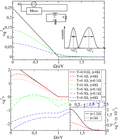
Figure 1: (color online) a) (top) Mesoscopic device coupled to a dissipative LC circuit. (bottom) typical histograms of the charge used to identify the noise and the third moment, at zero and finite voltage. Measured noise (damping parameter $\gamma$) at temperature $T=0.01\Omega$. No damping (full line), $\gamma/2=0.4\Omega$ (dashed line), $\gamma/2=0.6\Omega$ (dashed-dotted line). b) $T>\gamma/2$ (underdamped case). Inset: $T=0.01\Omega$ (over-damped regime).

Next, we introduce the inductive coupling between the mesoscopic circuit and the LC circuit $V_{int}=\alpha q\dot{I}$, where $\dot{I}$ is the time derivative of the current operator lesovik_loosen . This interaction is interpreted here as an external potential acting on the oscillator circuit. Because we are interested in calculating correlation functions of the LC circuit coordinate, we introduce a two-component auxiliary field $\eta$ (upper/lower contour) which allows to write the partition function:

$$\mathcal{Z}_{\eta}[I]=\int\mathcal{D}{\bf q}^{T}\exp i\Big{[}\frac{1}{2}{\bf q}^{T}\circ G^{-1}\circ{\bf q}-{\bf q}^{T}\sigma_{z}\circ(\alpha\dot{\bf I}+{\bf\eta})\Big{]}~{}.$$ (3)

The effective action is then quadratic in the oscillator coordinate, so that one can integrate out ${\bf q}$, and the effective action becomes (restoring integrals):

$$S_{eff} = -\frac{i}{2}\int dt\int dt^{\prime}({\bf\eta}(t)+\alpha\dot{\bf I}(t))^{T}\sigma_{z}\check{G}(t-t^{\prime})$$ (4)

$$~{}~{}~{}~{}~{}~{}\times\sigma_{z}({\bf\eta}(t^{\prime})+\alpha\dot{\bf I}(t^{\prime}))\Big{]}~{}.$$

The action of Eq. (4) is then used to compute the relevant averages by taking derivatives over the auxiliary field:

$$\langle q(t)\rangle=\frac{\alpha}{2}\sum_{s}\int d\tau\sigma_{z}^{s,s}(G^{+s}(t,\tau)+G^{-s}(t,\tau))$$

$$~{}~{}~{}~{}~{}~{}~{}~{}\times\langle\dot{I}(\tau^{s})Z[I]\rangle/\langle Z[I]\rangle~{},$$ (5)

$$\delta\langle q(t)q(0)\rangle=\alpha^{2}\sum_{s_{1},s_{2}}\sigma_{z}^{s_{1}s_{1}}\sigma_{z}^{s_{2}s_{2}}Z[I]^{-1}\int d\tau_{1}d\tau_{2}$$

$$~{}~{}~{}~{}\times\langle\dot{I}(\tau_{1}^{s_{1}})\dot{I}(\tau_{2}^{s_{2}})Z[I]\rangle G^{s_{1}+}(\tau_{1},0)G^{s_{2}-}(\tau_{2},t)~{},$$ (6)

with $Z[I]=\mathcal{Z}_{\eta=0}[I]$, and $\langle...\rangle$ denotes a non-equilibrium average over the mesoscopic system. In the above, we ignore contributions which originate from the zero point fluctuations of the LC circuit plus bath, as these are subtracted in the excess noise and third moment measurement which is implied in Fig 1. At this stage no approximation has been made on the magnitude of the inductive coupling. An expansion of the partition function in powers of $\alpha$ yields contributions for these averages which contain all high-order correlators of the current derivative moments. Such moments are translated into “regular” current correlators, using Fourier transforms. We start with noise, introducing the combination: $K^{\pm}(t)=\theta(t)(K^{>}(t)\pm K^{<}(t))$, where $K^{>}$ and $K^{<}$ are the off diagonal elements of $\langle\dot{I}(t^{s})\dot{I}(t^{\prime s^{\prime}})\rangle$ in Eq. (6). Going to the rotated Keldysh basis allows to rewrite the charge fluctuations at equal time as (the time dependance drops out):

$$\delta\langle q^{2}\rangle = \alpha^{2}\int\frac{d\omega}{2\pi}G^{R}(\omega)\{G^{K}(\omega)K^{-}(\omega)$$ (7)

$$-(G^{R}(\omega)-G^{A}(\omega))K^{+}(\omega)\}~{},$$

with the three non-vanishing Green’s oscillator function: $G^{R/A}(\omega)=[M(\omega^{2}-\Omega^{2})\pm i\textrm{sgn}(\omega)J(|\omega|)]^{-1}$ and $G^{K}=(2N(\omega)+1)(G^{R}(\omega)-G^{A}(\omega))$ ($N(\omega)$ is the Bose-Einstein distribution), were the spectral function of the bath $J(\omega)=\pi\sum_{n}\lambda_{n}^{2}/(2M_{n}\Omega_{n})\delta(\omega-\Omega_{n})$ gives rise to a finite line width for the LC circuit Green’s function.

Next, we relate the time derivative correlators to the current correlators: $K^{<}(\omega)=\omega^{2}S_{+}(\omega)$ and $K^{>}(\omega)=\omega^{2}S_{-}(\omega)$, with $S_{+}(\omega)=\int dt\langle I(0)I(t)\rangle e^{i\omega t}$ and $S_{-}(\omega)=S_{+}(-\omega)$, which correspond to the response function for emission/absorption of radiation from/to the mesoscopic circuit lesovik_loosen ; deblock_science . With these definitions, the final result for the measured excess noise reads:

$$\delta\langle q^{2}\rangle = 2\alpha^{2}\int_{0}^{\infty}\frac{d\omega}{2\pi}\omega^{2}[\chi^{\prime\prime}(\omega)]^{2}$$ (8)

$$~{}~{}\times\big{(}S_{+}(\omega)+N(\omega)(S_{+}(\omega)-S_{-}(\omega))\big{)}~{},$$

where $\chi^{\prime\prime}(\omega)=J(|\omega|)/[M^{2}(\omega^{2}-\Omega^{2})^{2}+J^{2}(|\omega|)$ is the susceptibility of Ref. caldeira , here generalized to arbitrary $J(|\omega|)$. Eq. (8) indicates that for a small line width, the integrand can be computed at the resonant frequency $\Omega$, and the measured noise is proportional to $S_{+}(\Omega)+N(\Omega)(S_{+}(\Omega)-S_{-}(\Omega))$, with a prefactor which diverges when the circuit is uncoupled to its environment lesovik_loosen . Eq. (8) constitutes a mesoscopic analog of the radiation line width calculation of larkin : a dissipative LC circuit cannot yield any divergences in the measured noise. Dissipation is essential in the measurement process.

Next, we turn to the measurement of the third moment. Performing a perturbative expansion in $\alpha$ of the average charge in Eq (5), only odd current (derivative) correlators can be generated in this series. The first term is proportional to $\langle\dot{I}\rangle$: it vanishes in a stationary situation (DC bias on the mesoscopic device). The next non-vanishing term is directly related to the third moment at finite frequencies: $L^{s_{1},s_{2},s_{3}}(t_{1},t_{2},t_{3})=\langle T_{K}\{\dot{I}(t_{1}^{s_{1}}\dot{I}(t_{2}^{s_{2}})\dot{I}(t_{3}^{s_{3}})\}\rangle$. The average charge is expressed in terms of the Green’s functions of the LC circuit plus bath and the current correlators.

$$\langle q\rangle_{(3)}=-\frac{i}{2}\alpha^{3}\int d\tau\theta(t-\tau)(G^{>}(t,\tau)-G^{<}(t,\tau))$$

$$\times\int dt_{1}dt_{2}\sum_{s_{1},s_{2}}\sigma_{z}^{s_{1}s_{1}}\sigma_{z}^{s_{2}s_{2}}G^{s_{1}s_{2}}(t_{1}-t_{2})L^{+s_{1}s_{2}}(\tau,t_{1},t_{2})~{}.$$ (9)

It turns out that the average charge can be expressed solely in terms of a special combination of current derivative correlators:

$$R^{\pm}(\tau,t_{1},t_{2}) = \theta(\tau-t_{1})\theta(t_{1}-t_{2})L^{\pm}(\tau,t_{1},t_{2})~{},$$ (10)

with

$$L^{\mp}(\tau,t_{1},t_{2}) = \left\langle\Big{[}[\dot{I}(\tau),\dot{I}(t_{1})]_{-},\dot{I}(t_{2})\Big{]}_{\mp}\right\rangle~{}.$$ (11)

That is, the mesoscopic circuit correlators appear only in the form of interlocked commutators ($-$)/anti-commutators ($+$). This is an important aspect of this scheme, because the commutator which is common for both correlators of Eq. (11) implies that our scheme is only effective when the transport is fully coherent, i.e. when the rate of escape for electrons from the mesoscopic device to the leads is large compared to the temperature. Such correlators vanish in the case of incoherent Coulomb blockade transport. Exploiting time translational invariance, the final result for the measured third moment then reads:

$$\langle q\rangle_{(3)} = -i\alpha^{3}\int_{-\infty}^{\infty}\frac{d\omega}{2\pi}G^{R}(0)\Big{[}G^{K}(\omega)R^{-}(0,\omega)$$ (12)

$$~{}~{}~{}~{}~{}~{}-(G^{R}(\omega)-G^{A}(\omega))R^{+}(0,\omega)\Big{]}~{},$$

Note the similarity between this expression and the one obtained in Eq. (7) for the measured noise. $R^{+}$ is weighted by same the spectral density of states of the LC oscillator plus bath $G^{R}-G^{A}$, as for the factor $K^{+}$ in Eq. (7). The factor $R^{-}$, on the other hand, does not contain the same frequencies as that of $K^{-}$ (see below). This result also shows which third moment correlator (which frequencies) the dissipative LC circuit is capable of measuring. Using the expressions of the oscillator circuit Green’s function:

$$\langle q\rangle_{(3)}=\frac{2\alpha^{3}}{M\Omega^{2}}\int_{0}^{\infty}d\omega\chi^{\prime\prime}(\omega)$$

$$~{}~{}~{}~{}\times\textrm{Re}\Big{\{}\Big{[}(2N(\omega)+1)R^{-}(0,\omega)-R^{+}(0,\omega)\Big{]}\Big{\}}~{},$$ (13)

There is a fundamental difference between the two responses of Eqs. (8) and (13). $\chi^{\prime\prime}(\omega)$ appears as a square in the measured noise (8), while it does not in the third moment (13). We next specify to strict ohmic or Markovian damping $J(\omega)=M\gamma\omega$, a memoryless bath being consistent with the adiabatic switching assumption. The limit of zero ohmic dissipation $\gamma\to 0$ leads to a divergence in the measured noise because it is proportional to the square of $\chi^{\prime\prime}(\omega)$: there are “large” charge fluctuations on the capacitor plates because it is pumping energy from the mesoscopic device. A finite damping is needed in order for the integral in Eq. (8) to converge: it explains the breakdown of adiabaticitylesovik_loosen . The measured third moment is not singular when $\gamma\to 0$.

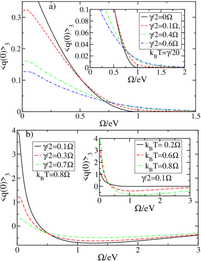
Figure 2: (color online) Measured third moment. a) $T\ll\gamma/2$ and $\gamma/2<\Omega$ for the displayed values of the damping parameter. Inset: zoom near $\Omega=eV$. b) case $\gamma/2<T$, at constant temperature and different value of $\gamma$. Inset: $\gamma$ is fixed and $T$ is varied.

Results are applied to a point contact. The excess noise is known to have a singular derivative at $\omega=eV$. $\langle q^{2}\rangle$ and $\langle q\rangle$ are plotted as a function of $\Omega/eV$, $\gamma/\Omega$, and $T/\Omega$, with $T$ the temperature of the LC circuit, which is assumed to be small compared to $eV$ (shot noise dominated regime) footnote . In the under-damped case the susceptibility $\chi^{\prime\prime}$ is a superposition of Lorentzian peaks at $\pm\Omega$ and width $\gamma$. Thus, if $\gamma\ll\Omega$ we expect qualitative behavior similar to that of the undamped case, which is indeed what happens, with the important result that the divergency is removed. Fig. 1a shows that at small temperature, the effect of damping is to wash out the singularity, and the measured noise flattens out. A curve with no damping is shown for comparison, after rescaling (it is infinite at $\omega=0$ for $\gamma\to 0$). The inset of Fig. 1b also applies to $T<\gamma$, but deals with the over damped regime: there is no reminiscence of the linear behavior found in the absence of damping because the two peaks of $\chi^{\prime\prime}(\omega)$ cannot be resolved, even at low temperatures. Fig. 1b shows the effect of the temperature on the noise both without and with dissipation, in the under damped regime. The measured noise can become negative at higher temperature because $S_{+}-S_{-}<0$, and because of the large population of LC oscillator states. Because we are considering excess effects (difference between the charge fluctuations with and without the applied bias) there is no controversy here. As in Fig. 1a, the cusps (or singularities), which survive for the undamped case even at these temperatures, are strongly attenuated due to damping. An important feature is that the measuring temperature $T$ enters our results exactly as in the undamped case, because the response function $\chi^{\prime\prime}(\omega)$ is temperature-independent ($\chi^{\prime\prime}(\omega)$ is related to the symmetrized correlation function of the damped HO via the fluctuaction-dissipation theorem).

We turn now to the measured third moment (Fig. 2). For $\gamma\to 0$, it does not have a singularity at $\omega=eV$, but it vanishes beyond this point, and has a linear behavior (not shown) close to $\omega=0$. For the under damped case $\gamma/2<\Omega$, the main effect is to reduce the amplitude of the measured third moment, and to wash out its vanishing at $\Omega=eV$ (see inset). Furthermore, one notices that the third moment saturates near $\omega=0$, and acquires a maximum in this region. The effect of temperature is displayed in Fig. 2: the structure at $\Omega=eV$ disappears, and the width of the maximum at $\omega=0$ is reduced. Similarly to the measured noise, the third moment can become negative either when the damping is increased (Fig. 2b), or when the temperature is increased (inset).

The above measurement setup and coupling conditions are easily achievable by on-chip inductive coupling to a SQUID circuit behaving as a harmonic oscillator. Recently reported quality factors of $\approx 100-150$, with an oscillator resonance of $\approx 3$GHz, and operating temperature $T\approx 25mk$ chiorescu_johansson correspond to the under damped regime discussed. A detailed investigation of the experimental setup will be reported elsewhere.

In summary, dissipation was included in the measurement of the higher current moments in the coherent regime; it is crucial to get a finite result for the noise. Third moment correlators have been identified with this scheme. The measurement of higher current moments, using the skewness and the sharpness of the charge histogram consitutes an extension.

T.M. and A.C. acknowledge support an ANR grant from the French ministry of research. E.P. thanks CPT for its hospitality. Discussions with G. Falci are gratefully acknowledged.

References

- (1) B. Reulet, J. Senzier, and D. E. Prober Phys. Rev. Lett. 91, 196601 (2003)
- (2) Yu. Bomze, G. Gershon, D. Shovkun, L. S. Levitov, and M. Reznikov Phys. Rev. Lett. 95, 176601 (2005)
- (3) T. Fujisawa, et al., Science 312, 1634 (5780); S. Gustavsson et al., Phys. Rev. Lett. 96, 076605 (2006). S. Gustavsson, R. Leturcq, T. Ihn, K. Ensslin, M. Reinwald, W. Wegscheider, cond-mat/0607192.
- (4) E. Onac, F. Balestro, L. H. W. van Beveren, U. Hartmann, Y. V. Nazarov, and L. P. Kouwenhoven Phys. Rev. Lett. 96, 176601 (2006); E. Onac, F. Balestro, B. Trauzettel, C. F. J. Lodewijk, and L. P. Kouwenhoven ibid. 96, 026803 (2006)
- (5) G. B. Lesovik and R. Loosen, Pis’ma Zh. Éksp. Teor. Fiz. 65, 280 (1997) [JETP Lett. 65, 295, (1997)]; U. Gavish, I. Imry, and Y. Levinson, Phys. Rev. B 62, 10637 (2000).
- (6) R. Aguado and L. P. Kouwenhoven, Phys. Rev. Lett. 84, 1986 (2000).
- (7) R. Deblock, E. Onac, L. Gurevich, and L. P. Kouvenhoven, Science 301, 203 (2003); P.-M. Billangeon, F.Pierre, H. Bouchiat, and R. Deblock, Phys. Rev. Lett. 96, 136804 (2006).
- (8) B. Trauzettel, I. Safi, F. Dolcini, and H. Grabert Phys. Rev. Lett. 92, 226405 (2004); A. V. Lebedev, A. Crépieux, and T. Martin, Phys. Rev. B 71, 075416 (2005).
- (9) C. W. J. Beenakker, M. Kindermann, and Yu. V. Nazarov, Phys. Rev. Lett. 90, 176802 (2003).
- (10) J. Tobiska and Yu. V. Nazarov Phys. Rev. Lett. 93, 106801 (2004); J. P. Pekola, ibid., 93, 206601 (2006); T. T. Heikkilä, P. Virtanen, G. Johansson, and F. K. Wilhelm ibid., 93, 247005 (2004); T. Ojanen and T. T. Heikkilä Phys. Rev. B 73, 020501 (2006); V. Brosco, R. Fazio, F. W. J. Hekking, and J. P. Pekola ibid., 74, 024524 (2006).
- (11) J. Gabelli, L.-H. Reydellet, G. Feve, J.-M. Berroir, B. Plaçais, P. Roche, and D. C. Glattli, Phys. Rev. Lett. 93, 056801 (2004).
- (12) A.I. Larkin and Yu. N. Ovchinikov, Zh. Eksp. Teor. Fiz. 53, 2159 (1967) [Sov. Phys. JETP 26, 1219 (1968)].
- (13) A. O. Caldeira and A. J. Leggett, Physica 121A, 587 (1983).
- (14) H. Grabert, P. Schramm, and G.-L. Ingold Phys. Rep. 168, 115 (1988).
- (15) When the current is amplified before being coupled to the LC circuit, this assumption can be relaxed, but additional filtering due to the amplifiers occurs.
- (16) I. Chiorescu et.al., Nature, 431, 159, (2004); J. Johansson et al., Phys. Rev. Lett., 96, 127006 (2006).