An Improved Initialization Procedure for the Density-Matrix Renormalization Group

Abstract

We propose an initialization procedure for the density-matrix renormalization group (DMRG): the recursive sweep method. In a conventional DMRG calculation, the infinite-algorithm, where two new sites are added to the system at each step, has been used to reach the target system size. We then need to obtain the ground state for a different system size for every site addition, so 1) it is difficult to supply a good initial vector for the numerical diagonalization for the ground state, and 2) when the system reduced to a 1D system consists of an array of nonequivalent sites as in ladders or Hubbard-Holstein model, special care has to be taken. Our procedure, which we call the recursive sweep method, provides a solution to these problems and in fact provides a faster algorithm for the Hubbard model as well as more complicated ones such as the Hubbard-Holstein model.

Introduction

After fifteen years since the density-matrix renormalization group (DMRG) [1, 2] was introduced as a new numerical method to obtain ground- and low-energy excited states for one-dimensional many-body systems, DMRG continues to enjoy its status as one of the most powerful numerical tools in condensed matter physics. It has been successfully applied to study various problems [3], which include correlated electron systems such as the Hubbard model [4, 5, 6] and the $t$-$J$ model [7], quantum systems at finite temperatures [8, 9, 10], quantum chemistry [11], quantum Hall systems [12], dynamical quantities [13, 14, 15]. The extreme accuracy obtained by DMRG in many cases has attracted interests for its mathematical reasons, and such viewpoint is also pursued vigorously (see, e.g., [16, 17]). One of the recent breakthroughs in the field is the development of several new methods to apply DMRG to real-time simulations of quantum systems [18, 19, 20]. Several review articles [21, 22, 23] describe the history of DMRG and its wide range of application.

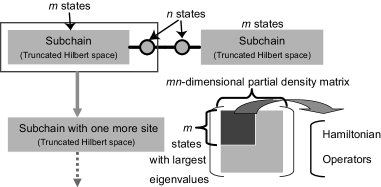
Figure 1: DMRG calculation. The one-dimensional lattice model is treated by iteratively adding sites to two subchains to construct superblocks from two subchains and two sites between them. In enlarging a subchain to contain one more site, the partial density matrix for the new block is calculated for the target state of the superblock. The eigenstates with $m$ largest eigenvalues are retained as the new basis for the enlarged subchain. The truncation error is assessed by calculating the sum $\eta$ of the eigenvalues for the discarded eigenstates. In the new basis, the matrix representations of the Hamiltonian and operators for the new block are calculated and stored for later use.

In DMRG, we consider a system consisting of sites aligned in a one-dimensional open-boundary chain. We systematically transform the Hilbert space of the system to one whose dimension is drastically reduced from the original one, while keeping the low-energy physics as unchanged as possible. In order to do this, we separate the system into parts, which we call blocks or subchains, and reduce the number of basis functions to describe the blocks, which we call the basis size for the blocks. What we actually do is to choose a basis that is fit to express one (or a few) quantum-mechanical state(s) of the original system (target state(s)), and expect that the low-energy excitations are recaptured in the chosen basis. The basis size to express physical states is reduced with the use of a partial density matrix calculated for some parts of a superblock, which is the whole or a partial chain and is usually constructed from two blocks and two sites. The part to calculate the partial density matrix is separated at some cut point from the rest of the system, which is called the environment block. While the number of states to be considered in an exact diagonalization increases exponentially with the number of sites, the contribution of high-energy configurations to the low-energy physics is usually exponentially small. With the use of the DMRG algorithm, most important states can be systematically found. In many cases, the dimension of the Hilbert space can be kept much smaller than in the exact diagonalization, and almost exact results can be obtained with moderate computational efforts.

In DMRG we need to start with a warm-up process, which is the process to iteratively add new sites to one or more subchains, until the Hilbert space of the system with the desired number of sites can be represented with the reduced basis. If the system consists of homogeneous sites, we can just add two new sites between two subchains of the same length $l$ to make a superblock of $2l+2$ sites in order to obtain a subchain that has $l+1$ sites, and repeat this until the superblock acquires the desired number of sites. This process is called the infinite algorithm DMRG; we can repeat the addition of a site to the subchain indefinitely. Once this warm-up procedure has finished, we can enhance the quality of the basis by systematically moving the cut location back and forth within the chain (the finite algorithm DMRG).

In this letter, we focus on the warm-up process. When we increase the number of sites by two in the infinite-algorithm, it is in general difficult to supply a good initial vector for the numerical diagonalization for the target state, so usually a random vector is plugged. Our new procedure reduces the number of numerical diagonalization from a random vector, with the use of the finite algorithm DMRG.

Method

We illustrate the new procedure for the case of $N_{c}$ original sites per full site. Our idea here is to modify the infinite algorithm in the conventional DMRG, which adds two sites at the center of the superblock at each step, so that two full sites are added at the center of the superblock per cycle. As we elaborate in the below, for each of the left and right subchains, we retain $N_{c}$ subchains that have respectively $0,1,\ldots,N_{c}-1$ original sites besides $n$ full sites, instead of just one subchain each. The longest subchain among the left subchains and the longest among the right ones are used to construct a new superblock, and with the use of the finite algorithm, those subchains are enlarged by $1,2,\ldots,N_{c}$ original sites. Then we can repeat the same process for a superblock that is two full sites longer.

Now we explain how this can be done. We align the original sites in a one-dimensional chain so that the same kind of sites appear periodically along the chain, as

$$\cdots\mbox{{) --- (b}}_{0}\mbox{{---}}\cdots\mbox{{---b}}_{N_{c}-1}\mbox{{) --- (b}}_{0}\mbox{{---}}\cdots\mbox{{---b}}_{N_{c}-1}\mbox{{) --- (}}\cdots,$$

where the original sites are denoted as b₀, …,b${}_{N_{c}-1}$, and each full site is enclosed in ($\cdots$).

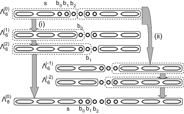
Figure 2: The recursive sweep method illustrated for the case of $n=2$ and $N_{c}=3$. A full site, s, is represented as an oval, and an original site, $\textsf{b}_{i}$, as a circle. An arrow shows how an original site is added to a subchain, which is represented as a round cornered rectangle. The first steps to enlarge the left and right subchains are marked as (i) and (ii), as in the text. For the definition of the superblocks $\Lambda_{6}^{(0,\pm 1,\pm 2)}$ and $\Lambda_{8}^{(0)}$, see the text.

We denote the full site as s, and a sequence of $n$ full sites as sⁿ. Suppose we have the left and right subchains $L_{n,i}$ and $R_{n,i}$ ($i=0,1,\ldots,N_{c}-1$) respectively,
$L_{n,0}=\textsf{s}^{n}$, $R_{n,0}=\textsf{s}^{n}$,
$L_{n,1}=\textsf{s}^{n}$—b₀, $R_{n,1}=$ b${}_{N_{c}-1}$—$\textsf{s}^{n}$,
$L_{n,2}=\textsf{s}^{n}$—b₀—b₁, $R_{n,2}=$ b${}_{N_{c}-2}$—b${}_{N_{c}-1}$—$\textsf{s}^{n}$,
…,
$L_{n,N_{c}-1}=\textsf{s}^{n}$—b₀—$\cdots$—b${}_{N_{c}-1}$, and
$R_{n,N_{c}-1}=$ b₁—$\cdots$—b${}_{N_{c}-2}$—b${}_{N_{c}-1}$—$\textsf{s}^{n}$,
where $L_{n,i}$ ($R_{n,i}$) has (a) $n$ full sites from the left(right) edge of the original chain and (b) $i(=0,1,\ldots,N_{c}-1)$ original sites from the $(n+1)$-th site $s_{n}$ ($s_{L-n-1}$). We enlarge $L_{n,N_{c}-1}$ and $R_{n,N_{c}-1}$ by $N_{c}$ original sites to obtain $2N_{c}$ subchains $L_{n+1,i}$ and $R_{n+1,i}$ ($i=0,1,\ldots,N_{c}-1$) as follows.

First, we construct a superblock $\Lambda_{2n+2}^{(0)}$ that has $2n+2$ full sites:

$$\Lambda_{2n+2}^{(0)}=L_{n,N_{c}-1}\mbox{{---b}}_{N_{c}-1}(p_{\alpha})\mbox{{---b}}_{0}(p_{\beta})\mbox{{---}}R_{n,N_{c}-1}$$

is constructed from $L_{n,N_{c}-1}$, two sites $p_{\alpha}$ and $p_{\beta}$, and $R_{n,N_{c}-1}$, aligned in this order from the left. We calculate the target state(s) for $\Lambda_{2n+2}^{(0)}$. Then we can obtain (i) $L_{n+1,0}$ by calculating the partial density matrix for $L_{n,N_{c}-1}$ and $p_{\alpha}$ combined, and in the same way, (ii) $R_{n+1,0}$ from $p_{\beta}$ and $R_{n,N_{c}-1}$ combined. We write this as

$$\mbox{(i) \sf[}L_{n,N_{c}-1}\mbox{{---b}}_{N_{c}-1}(p_{\alpha})\mbox{{]}}\rightarrow L_{n+1,0},$$

and

$$\mbox{(ii)}R_{n+1,0}\leftarrow\mbox{{[b}}_{0}(p_{\beta})\mbox{{---}}R_{n,N_{c}-1}\mbox{{]}}.$$

Next, as in the finite algorithm, we move the cut location to the right by one original site. This is possible because we have $R_{n,N_{c}-2}$. The new superblock, $\Lambda_{2n+2}^{(1)}$ also has $2n+2$ full sites:

$$\Lambda_{2n+2}^{(1)}=L_{n+1,0}\mbox{{---b}}_{0}(p_{\beta})\mbox{{---b}}_{1}(p_{\gamma})\mbox{{---}}R_{n,N_{c}-2}$$

is constructed from $L_{n+1,0}$, two original sites $p_{\beta}$ and $p_{\gamma}$, and $R_{n,N_{c}-2}$. Then we obtain $L_{n+1,1}$ by calculating the partial density matrix for $L_{n+1,0}$ and $p_{\beta}$ combined:

$$\mbox{{[}}L_{n+1,0}\mbox{{---b}}_{0}(p_{\beta})\mbox{{]}}\rightarrow L_{n+1,1}.$$

This can be repeated $N_{c}-2$ more times, where for each $i$ ($i=2,\ldots,N_{c}-1$), we obtain $L_{n+1,i}$ from the superblock $\Lambda_{2n+2}^{(i)}$ that is constructed from $L_{n+1,i-1}$, two original sites, and $R_{n,N_{c}-1-i}$:

$$\Lambda_{2n+2}^{(i)}=L_{n+1,i-1}\mbox{{---b}}_{i-1}\mbox{{---b}}_{i}\mbox{{---}}R_{n,N_{c}-1-i},$$

$$\mbox{{[}}L_{n+1,i-1}\mbox{{---b}}_{i-1}\mbox{{]}}\rightarrow L_{n+1,i}.$$

Also, by moving the cut location to the left $N_{c}-1$ times, we make superblocks $\Lambda_{2n+2}^{(-i)}$ ($i=1,\ldots,N_{c}-1$) that consists of $L_{n+1,N_{c}-1-i}$, two original sites and $R_{n,i-1}$, to obtain $R_{n+1,i}$ ($i=1,\ldots,N_{c}-1$):

$$\Lambda_{2n+2}^{(-i)}=L_{n,N_{c}-1-i}\mbox{{---b}}_{N_{c}-1-i}\mbox{{---b}}_{N_{c}-i}\mbox{{---}}R_{n+1,i-1},$$

$$R_{n+1,i}\leftarrow\mbox{{[b}}_{N_{c}-i}\mbox{{---}}R_{n+1,i-1}\mbox{{]}},$$

for $i=1,\ldots,N_{c}-1$.

In these steps, the initial vector for each of the exact diagonalizations can be calculated from the target state obtained in the most recent step (for $\Lambda_{2n+2}^{(-1)}$, we use the target state for $\Lambda_{2n+2}^{(0)}$, rather than $\Lambda_{2n+2}^{(+N_{c}-1)}$). The calculations for $\{L_{n+1,i}\}$ and $\{R_{n+1,i}\}$ can be done without data dependence to each other in a parallel computer.

Now we have $L_{n+1,i}$ ($i=0,\ldots,N_{c}-1$) and $R_{n+1,i}$ ($i=0,\ldots,N_{c}-1$), so we have enlarged the subchains by one full site. We have to obtain the target states from random vectors only once. This procedure can be repeated for the incremented values of $n$, until the superblock has all the $L$ full sites.

Note that, because DMRG limits the number of the basis functions to $m$ to describe finite-size blocks, a calculation with any choice of basis should converge to the result of the exact diagonalization in the $m\rightarrow\infty$ limit. The questions here are:

• how fast the calculation converges, and

• whether we can calculate with enough accuracy within a practical computation time.

We also note that the recursive sweep method described here is different from (a) the initialization by Liang and Pang [24] for a rectangle lattice where the ratio of horizontal and vertical hopping parameters is controlled through several finite-algorithm sweeps that involve the whole system, (b) the warm-up with a conventional numerical renormalization group [25] by Xiang [5], the two-step DMRG by Moukouri and Caron [26], and (c) the quantum information entropy-based approach by Legeza and Sólyom [27].

Choice of targets

Because environment blocks are shorter than the enlarged block in the finite-algorithm steps, it is advisable to target several states having different quantum numbers (e.g., numbers of up-spin electrons and down-spin electrons) near the target state. In calculating for the half-filled, $L$-site system ($L$: an even integer), we target not only the ground state for $(n_{\uparrow},n_{\downarrow})=(L/2,L/2)$ but also the ground states for $(n_{\uparrow}+d_{\uparrow,j},n_{\downarrow}+d_{\downarrow,j^{\prime}})$ ($d_{j},d_{j^{\prime}}=0,\pm 1$).

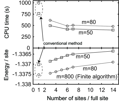
Figure 3: Upper panel: The CPU time for the warm-up for the 84-site Hubbard model with $U/t=2$, for the number of retained eigenstates $m=30,50,80$, as function of the number of sites in a full site for the recursive sweep method. The calculations were conducted on a workstation with two Xeon 5160 chips and 4GB of RAM. Lower panel: The ground-state energy per site at the end of the warm-up for the 84-site Hubbard model with $U/t=2$, for the number of retained eigenstates $m=50,80$, as function of the number of sites in a full site for the recursive sweep method. The result for the conventional infinite method is also shown. The true energy, which can be estimated with the finite-algorithm DMRG with a large $m=800$, is $-1.337~{}785~{}42$ and shown as a dotted line. Other lines are guide to the eye. The ground state energy per site for the infinite-length Hubbard model with $U=2$, obtained with the exact solution by Lieb and Wu, is $-1/2-\int_{-\infty}^{\infty}J_{0}(x)J_{1}(x)/x(1+e^{|x|}){\rm d}x=-1.344~{}374~{}34$.

Results

The Hubbard model

We first apply the recursive sweep method to the half-filled Hubbard chain with homogeneous sites,

$$H=-\sum_{i,\sigma}t(c_{i,\sigma}^{\dagger}c_{i+1,\sigma}+\mbox{H.c.})+\sum_{i}U(n_{i,\uparrow}-1)(n_{i,\downarrow}-1),$$ (1)

by considering multiple sites as one composite full site. In each iteration of the recursive sweep method, we add two composite sites to the superblock. When the length of the superblock equals or exceeds the desired length $L_{0}$, we can stop the recursive sweep method and start the finite-algorithm sweeps.

As shown in Figure 3, the time required for the warm-up stage is almost halved in the case of the 84-site Hubbard model with $U/t=2$ by the use of this method. The longer cycle we take, generally the faster the calculation becomes. We also plot the ground state energy per site in Figure 3. The ground state energy becomes slightly worse than in the conventional infinite-algorithm warm-up with the same number of retained states $m=50$. When we increase $m$ to $m=80$, however, the energy becomes better than in the infinite-algorithm with $m=50$ for up to seven sites per cycle, while the CPU time spent is still significantly lower. So a small increase in $m$ can compensate the increased error due to the use of the recursive sweep algorithm with $N_{c}=2-7$.

The Hubbard-Holstein model

When the system is a repetition of three or more types of sites, as in the case of the pseudo-site method for the Holstein phonons [28] or multi-leg ladder systems, the choice of the warm-up process in DMRG is not obvious. Hereafter, we call one original site, which becomes the period of the repetition of the (pseudo-)sites, as a full site. (a) If we enlarge the two subchains in a mirror-symmetric way, at most of the steps, we have two incomplete full sites at the center of the superblock. Then the environment for the new sites at the center is much different from the later stages of the calculation, when the full site is completely within the superblock. (b) Alternatively, we can increase the length of the subchain that starts from one edge of the chain by iteratively using short subchains whose whole basis can be exactly treated, in a way in which the sites in the superblock constitute a number of full sites at each step. In this case the new sites are always added near the edge of the chain, even when they are around the center of the original system. So both of the approaches (a)(b) have shortcomings that should deteriorate the choice of the reduced basis, which can be overcome with the use of the recursive sweep method as follows.

Here we consider the Hubbard-Holstein model [29] on a one-dimensional chain,

$$\begin{split}H&=-\sum_{i,\sigma}t(c_{i,\sigma}^{\dagger}c_{i+1,\sigma}+\mbox{h.c.})+\sum_{i}Un_{i,\uparrow}n_{i,\downarrow}\\ &+\sum_{i,\sigma}gn_{i,\sigma}(a_{i}+a_{i}^{\dagger})+\sum_{i}\hbar\omega_{0}a_{i}^{\dagger}a_{i}.\end{split}$$ (2)

Here, $c_{i,\sigma}$ annihilates an electron with spin $\sigma(=\uparrow,\downarrow)$ at site $i$, $n_{i,\sigma}=c_{i,\sigma}^{\dagger}c_{i,\sigma}$ is the electron number, $g$ is the electron-phonon coupling, and $a_{i}$ is the phonon annihilator at site $i$. For the application of the pseudo-site method to the Hubbard-Holstein model, the present author, in a collaboration with Arita and Aoki [30], has previously come up with another method, the compensation method, to make improve the choice of basis for the infinite-algorithm warm-up. Because DMRG is a variational method, the calculated ground state energy is always higher than the actual value; the lower energy means the better convergence.

As we show in Figure 4, the recursive sweep method warm-up (solid circle in the plot) results in a much better energy per site that does not fluctuate and continues to decrease as the number of full sites in the left subchain is increased. Similar results have also been observed for other parameter sets.

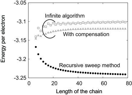
Figure 4: The energy per electron in units of $t$ against the length of the chain at intermediate stages of the warm-up process, calculated (i) with the infinite algorithm without the compensation method, (ii) with the infinite algorithm with the compensation method, and (iii) with the recursive sweep method, for the Hubbard-Holstein model with $(U/t,g/t,\omega_{0}/t)=(2,3,5)$. $2^{N_{b}}$=16 is chosen for the cutoff in the phonon number. The size of the basis is $m=70$ for all the calculations. The memory required for the calculation is around 700MB for the recursive sweep method, when all subchains and operators for calculation of various correlation functions are retained for later use.

Summary

The recursive sweep algorithm allows an initialization of a DMRG calculation when the system is a repetition of multiple kinds of sites, without the need of treating incomplete cycles of sites or the need of adding new sites at locations much off the center of a superblock. It is an extention of the infinite algorithm DMRG by the finite algorithm sweeps, over one cycle of added sites to both directions along the chain, whose computational cost is much smaller than in the conventional infinite algorithm. We have demonstrated that the present algorithm improves the calculation for a system of local phonons coupled to correlated electrons compared to our previous method. The recursive sweep algorithm is also applicable to a chain with homogeneous sites. We have demonstrated that we can both reduce the calculation time and improve the energy when we apply the algorithm with a small increase in the number of retained states.

References

- [1] S. R. White, Phys. Rev. Lett. 69, 2863 (1992).
- [2] S. R. White, Phys. Rev. B 48, 10345 (1993).
- [3] I. Peschel, X. Wang, M. Kaulke, and K. Hallberg, eds., Density-Matrix Renormalization — A new numerical method in physics — (Springer Berlin, 1999).
- [4] R. M. Noack, S. R. White, and D. J. Scalapino, Phys. Rev. Lett. 73, 882 (1994).
- [5] T. Xiang, Phys. Rev. B 53, R10445 (1996).
- [6] R. Arita, K. Kuroki, H. Aoki, and M. Fabrizio, Phys. Rev. B 57, 10324 (1998).
- [7] S. R. White and D. J. Scalapino, Phys. Rev. Lett. 80, 1272 (1998).
- [8] R. J. Bursill, T. Xiang, and G. A. Gehring, J. Phys.: Cond. Mat. 8, L583 (1996).
- [9] N. Shibata, J. Phys. Soc. Jpn 66, 2221 (1997).
- [10] X. Wang and T. Xiang, Phys. Rev. B 56, 5061 (1997).
- [11] S. R. White, J. Chem. Phys. 117, 7472 (2002).
- [12] N. Shibata and D. Yoshioka, Phys. Rev. Lett. 86, 5755 (2001).
- [13] K. A. Hallberg, Phys. Rev. B 52, R9827 (1995).
- [14] T. D. Kühner and S. R. White, Phys. Rev. B 60, 335 (1999).
- [15] E. Jeckelmann, Phys. Rev. B 66, 045114 (2002).
- [16] F. Verstraete, D. Porras, and J. I. Cirac, Phys. Rev. Lett. 93, 227205 (2004).
- [17] Ö. Legeza and J. Sólyom, Phys. Rev. B 70, 205118 (2004).
- [18] M. A. Cazalilla and J. B. Marston, Phys. Rev. Lett. 88, 256403 (2002).
- [19] G. Vidal, Phys. Rev. Lett. 93, 040502 (2004).
- [20] S. R. White and A. E. Feiguin, Phys. Rev. Lett. 93, 076401 (2004).
- [21] U. Schollwöck, Rev. Mod. Phys. 77, 259 (2005).
- [22] G. De Chiara, M. Rizzi, D. Rossini, and S. Montangero, cond-mat/0603842.
- [23] K. Hallberg, Adv. Phys. 55, 477 (2006).
- [24] S. Liang and H. Pang, Phys. Rev. B 49, 9214 (1994).
- [25] K. G. Wilson, Rev. Mod. Phys. 47, 773 (1975).
- [26] S. Moukouri and L. G. Caron, Phys. Rev. B 67, 092405 (2003).
- [27] Ö. Legeza and J. Sólyom, Phys. Rev. B 68, 195116 (2003).
- [28] E. Jeckelmann and S. R. White, Phys. Rev. B 57, 6376 (1998).
- [29] M. Tezuka, R. Arita, and H. Aoki, Phys. Rev. Lett. 95, 226401 (2005), and references therein.
- [30] M. Tezuka, R. Arita, and H. Aoki, Physica B 359, 708 (2005).