Why do ultrasoft repulsive particles cluster and crystallize?
Analytical results from density functional theory

Abstract

We demonstrate the accuracy of the hypernetted chain closure and of the mean-field approximation for the calculation of the fluid-state properties of systems interacting by means of bounded and positive-definite pair potentials with oscillating Fourier transforms. Subsequently, we prove the validity of a bilinear, random-phase density functional for arbitrary inhomogeneous phases of the same systems. On the basis of this functional, we calculate analytically the freezing parameters of the latter. We demonstrate explicitly that the stable crystals feature a lattice constant that is independent of density and whose value is dictated by the position of the negative minimum of the Fourier transform of the pair potential. This property is equivalent with the existence of clusters, whose population scales proportionally to the density. We establish that regardless of the form of the interaction potential and of the location on the freezing line, all cluster crystals have a universal Lindemann ratio $L_{\rm f}=0.189$ at freezing. We further make an explicit link between the aforementioned density functional and the harmonic theory of crystals. This allows us to establish an equivalence between the emergence of clusters and the existence of negative Fourier components of the interaction potential. Finally, we make a connection between the class of models at hand and the system of infinite-dimensional hard spheres, when the limits of interaction steepness and space dimension are both taken to infinity in a particularly described fashion.

I Introduction

Cluster formation in complex fluids is a topic that has attracted considerable attention recently.sear ; fs1 ; fs2 ; bartlett1 ; bartlett2 ; lr1 ; lr2 ; jpcm ; epl The general belief is that a short-range attraction in the pair interaction potential is necessary to initiate aggregation and a long-range repulsive tail in order to limit cluster growth and prevent phase separation. An alternative scenario for cluster formation pertains to systems whose constituent particles interact by means of purely repulsive potentials. Cluster formation in this case is counterintuitive at first sight: why should particles form clusters if there is no attraction acting between them? The answer lies in an additional property of the effective repulsion, namely that of being bounded, thus allowing full particle overlaps. Though surprising and seemingly unphysical at first, bounded interactions are fully legitimate and natural as effective potentialslikos:pr:01 between polymeric macromolecular aggregates of low internal monomer concentration, such as polymers,krueger:89 ; hall:94 ; louis:prl:00 dendrimers,ingo:jcp:04 ; ballik:ac:04 microgels,denton:03 ; gottwald:04 ; gottwald:05 or coarse-grained block copolymers.pierleoni:prl:06 ; hansen:molphys:06 The growing interest in this type of effective interactions is also underlined by the recent mathematical proof of the existence of crystalline ground states for such systems.suto:prl:05 ; suto:prb:06

Cluster formation in the fluid and in the crystal phases was explicitly seen in the system of penetrable spheres, following early simulation resultsklein:94 and subsequent cell-model calculations.pensph:98 Cluster formation was attributed there to the tendency of particles to create free space by forming full overlaps. The conditions under which ultrasoft and purely repulsive particles form clusters have been conjectured a few years agocriterion and explicitly confirmed by computer simulation very recently.bianca:prl:06 The key lies in the behavior of the Fourier transform of the effective interaction potential: for clusters to form, it must contain negative parts, forming thus the class of $Q^{\pm}$-interactions. The complementary class of potentials with purely nonnegative Fourier transforms, $Q^{+}$, does not lead to clustering but to remelting at high densities.stillinger:physica ; likos:gauss ; saija1 ; saija2 ; saija3 ; archer An intriguing feature of the crystals formed by $Q^{\pm}$-systems is the independence of the lattice constant on density,criterion ; bianca:prl:06 a feature that reflects the flexibility of soft matter systems in achieving forms of self-organization unknown to atomic ones.daan:nature ; daan:web The same characteristic has recently been seen also in slightly modified models that contain a short-range hard core.primoz:07 In this work, we provide an analytical solution of the crystallization problem and of the properties of the ensuing solids within the framework of an accurate density functional approach. We explicitly demonstrate the persistence of a single length scale at all densities and for all members of the $Q^{\pm}$-class and offer thus broad physical insight into the mechanisms driving the stability of the clustered crystals. We further establish some universal structural properties of all $Q^{\pm}$-systems both in the fluid and in the solid state, justifying the use of the mean-field density functional on which this work rests. We make a connection between our results and the harmonic theory of solids in the Einstein-approximation. Finally, we establish a connection with suitably-defined infinite dimensional models of hard spheres.

The rest of this paper is organized as follows: in Sec. II we derive an accurate density functional by starting with the uniform phase and establishing the behavior of the direct correlation functions of the fluid with density and temperature. Based on this density functional, we perform an analytical calculation of the freezing characteristics of the $Q^{\pm}$-systems by employing a weak approximation in Sec. III. The accuracy of this approximation is successfully tested against full numerical minimization of the functional in Sec. IV. In Sec. V the equivalence between the density functional and the theory of harmonic crystals is demonstrated, whereas in Sec. VI a connection is made with inverse-power potentials. Finally, in Sec. VII we summarize and draw our conclusions. Some intermediate, technical results that would interrupt the flow of the text are relegated in the Appendix.

II Density functional theory

II.1 Definition of the model

In this work, we focus our interest on systems of spherosymmetric particles interacting by means of bounded pair interactions $v(r)$ of the form:

$$v(r)=\epsilon\phi(r/\sigma),$$ (1)

with an energy scale $\epsilon$ and a length scale $\sigma$, and which fulfill the Ruelle conditions for stability.Ruelle:book In Eq. (1) above, $\phi(x)$ is some dimensionless function of a dimensionless variable and $r$ denotes the distance between the spherosymmetric particles. In the context of soft matter physics, $v(r)$ is an effective potential between, e.g., the centers of mass of macromolecular entities, such as polymer chains or dendrimers.ballik:ac:04 As the centers of mass of the aggregates can fully overlap without this incurring an infinitely prohibitive cost in (free) energy, the condition of boundedness is fulfilled:

$$0\leq v(r)<K,$$ (2)

with some constant $K$.

The interaction range is set by $\sigma$, typically the physical size (e.g., the gyration radius) of the macromolecular aggregates that feature $v(r)$ as their effective interaction. In addition to being bounded, the second requirement to be fulfilled by the function $\phi(x)$ is that it decay sufficiently fast to zero as $x\to\infty$, so that its Fourier transform $\tilde{\phi}(y)$ exists. In three spatial dimensions, we have

$$\tilde{\phi}(y)=4\pi\int_{0}^{\infty}{\rm d}x\,\frac{\sin(yx)}{yx}x^{2}\phi(x)$$ (3)

and, correspondingly,

$$\tilde{v}(k)=\epsilon\sigma^{3}\tilde{\phi}(k\sigma)$$ (4)

for the Fourier transform $\tilde{v}(k)$ of the potential, evaluated at wavenumber $k$. Our focus in this work is on systems for which $\tilde{v}(k)$ is oscillatory, i.e., $v(r)$ features positive and negative Fourier components, classifying it as a $Q^{\pm}$-potential.criterion Though this work is general, for the purposes of demonstration of our results, we consider a particular realization of $Q^{\pm}$-potentials, namely the generalized exponential model of exponent $m$, (GEM-$m$):

$$v(r)=\epsilon\exp[-(r/\sigma)^{m}],$$ (5)

with $m=4$. It can be shown that all members of the GEM-$m$ family with $m>2$ belong to the $Q^{\pm}$-class, see Appendix A.

A short account of the freezing and clustering behavior of the GEM-4 model has been recently published.bianca:prl:06 Another prominent member of the family is the $m=\infty$ model, which corresponds to penetrable spheresklein:94 ; pensph:98 ; fernaud with a finite overlap energy penalty $\epsilon$. Indeed, the explicitly calculated phase behavior of these two show strong resemblances, with the phase diagram of both being dominated by the phenomenon of formation of clusters of overlapping particles and the subsequent ordering of the same in periodic crystalline arrangements.pensph:98 ; fernaud In this work, we provide a generic, accurate, and analytically tractable theory of inhomogeneous phases of $Q^{\pm}$-systems.

II.2 The uniform fluid

Let us start from the simpler system of a homogeneous fluid, consisting of $N$ spherosymmetric particles enclosed in a macroscopic volume $V$. The structure and thermodynamics of the system are determined by the density $\rho=N/V$ and the absolute temperature $T$ or, better, their dimensionless counterparts:

$$\rho^{*}\equiv\rho\sigma^{3}$$

and

$$T^{*}\equiv\frac{k_{\rm B}T}{\epsilon},$$

with Boltzmann’s constant $k_{\rm B}$. As usual, we also introduce for future convenience the inverse temperature $\beta=(k_{\rm B}T)^{-1}$. We seek for appropriate and accurate closures to the Ornstein-Zernike relationhansen:book

$$h(r)=c(r)+\rho\int{\rm d}^{3}r^{\prime}c(|{\bf r}-{\bf r^{\prime}}|)h(r^{\prime}),$$ (6)

connecting the total correlation function $h(r)$ to the direct correlation function $c(r)$ of the uniform fluid. One possibility is offered by the hypernetted chain closure (HNC) that reads ashansen:book

$$h(r)=\exp\left[-\beta v(r)+h(r)-c(r)\right]-1.$$ (7)

An additional closure, the mean-field approximation (MFA), was also employed and will be discussed later.

Our solution by means of approximate closures was accompanied by extensive $NVT$-Monte Carlo (MC) simulations. We measured the radial distribution function $g(r)\equiv h(r)+1$ as well as the structure factor $S(k)=1+\rho{\tilde{h}}(k)$, where ${\tilde{h}}(k)$ is the Fourier transform of $h(r)$, to provide an assessment of the accuracy of the approximate theories. We typically simulated ensembles of up to $3\,000$ particles for a total of $150\,000$ Monte Carlo steps. Measurements were taken in every tenth step after equilibration.

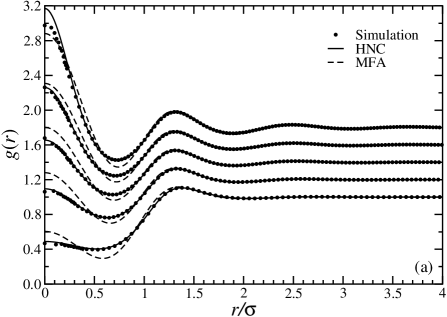
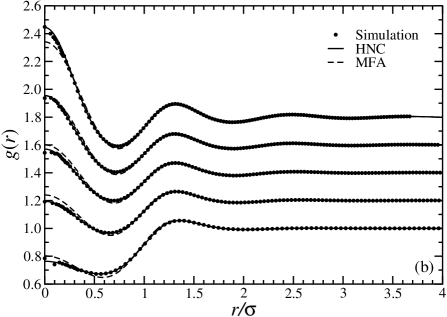
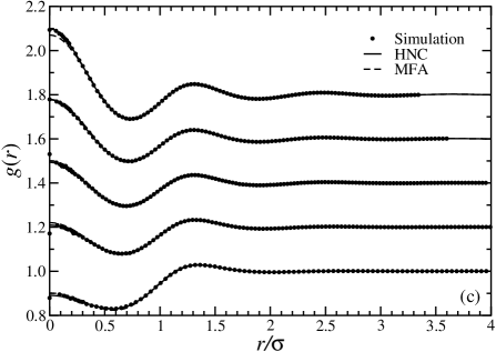
Figure 1: Radial distribution functions $g(r)$ of the GEM-4 model as obtained by Monte Carlo simulation (points), the HNC-closure (solid lines) and the MFA (dashed lines), at various temperatures and densities. For clarity, the curves on every panel have been shifted upwards by certain amounts, which are given below in square brackets, following the value indicating the density $\rho^{*}$. (a) $T^{*}=0.5$ and densities, from bottom to top: $\rho^{*}=0.5$ [0]; $\rho^{*}=1.0$ [0.2]; $\rho^{*}=1.5$ [0.4]; $\rho^{*}=2.0$ [0.6]; $\rho^{*}=2.5$ [0.8]. (b) $T^{*}=1.0$ and densities, from bottom to top: $\rho^{*}=1.0$ [0]; $\rho^{*}=2.0$ [0.2]; $\rho^{*}=3.0$ [0.4]; $\rho^{*}=4.0$ [0.6]; $\rho^{*}=5.0$ [0.8]. (c) $T^{*}=2.0$ and densities, from bottom to top: $\rho^{*}=2.0$ [0]; $\rho^{*}=4.0$ [0.2]; $\rho^{*}=6.0$ [0.4]; $\rho^{*}=8.0$ [0.6]; $\rho^{*}=10.0$ [0.8].

In Fig. 1 we show comparisons for the function $g(r)$ as obtained from the MC simulations and from the HNC closure for a variety of temperatures and densities. It can be seen that agreement between the two is obtained, to a degree of quality that is excellent. Tiny deviations between the HNC and MC results appear only at the highest density and for a small region around $r=0$ for low temperatures, $T^{*}=0.5$. Otherwise, the system at hand is described by the HNC with an extremely high accuracy and for a very broad range of temperatures and densities. We note that, although in Fig. 1 we restrict ourselves to temperatures $T^{*}\leq 2.0$, the quality of the HNC remains unaffected also at higher temperatures.criterion

In attempting to gain some insight into the remarkable ability of the HNC to describe the fluid structure at such a high level of accuracy, it is useful to recast this closure in density-functional language. Following the famous Percus idea,hansen:book ; percus:62 ; percus:64 ; denton:pra:91 ; yethiraj:jcp:01 the quantity $\rho g(r)$ can be identified with the nonuniform density $\rho(r)$ of an inhomogeneous fluid that results when a single particle is kept fixed at the origin, exerting an ‘external’ potential $V_{\rm ext}(r)=v(r)$ on the rest of the system. Following standard procedures from density functional theory, we find that the sought-for density profile $\rho(r)$ is given by

$$\rho(r)=\Lambda^{-3}\exp\left\{\beta\mu-\beta v(r)-\frac{\delta\beta F_{\rm ex}[\rho]}{\delta\rho(r)}\right\},$$ (8)

where $\Lambda$ is the thermal de Broglie wavelength and $\mu$ the chemical potential associated with average density $\rho$ and temperature $T$. Moreover, $F_{\rm ex}[\rho]$ is the intrinsic excess free energy, a unique functional of the density $\rho(r)$. As such, $F_{\rm ex}[\rho]$ can be expanded in a functional Taylor series around its value for a uniform liquid of some (arbitrary) reference density $\rho_{0}$. For the problem at hand, $\rho_{0}=\rho$ is a natural choice and we obtainsingh

$$\beta F_{\rm ex}[\rho]=\beta F_{\rm ex}(\rho) - \sum_{n=1}^{\infty}\frac{1}{n!}\int\int\cdots\int{\rm d}^{3}r_{1}{\rm d}^{3}r_{2}\ldots{\rm d}^{3}r_{n}$$ (9)

$$\times c_{0}^{(n)}({\bf r}_{1},{\bf r}_{2},\ldots,{\bf r}_{n};\rho)$$

$$\times \Delta\rho({\bf r}_{1})\Delta\rho({\bf r}_{2})\ldots\Delta\rho({\bf r}_{n}),$$

where $F_{\rm ex}(\rho)$ denotes the excess free energy of the homogeneous fluid, as opposed to that of the inhomogeneous fluid, $F_{\rm ex}[\rho]$, and

$$\Delta\rho({\bf x})\equiv\rho({\bf x})-\rho.$$ (10)

The basis of the expansion given by Eq. (9) above is the fact that $F_{\rm ex}[\rho]$ is the generating functional for the hierarchy of the direct correlation functions (dcf’s) $c_{0}^{(n)}$. In particular, $-\beta^{-1}c_{0}^{(n)}$ is the $n$-th functional derivative of the excess free energy with respect to the density field, evaluated at the uniform density $\rho$:singh ; evans:78

$$c_{0}^{(n)}({\bf r}_{1},{\bf r}_{2},\ldots,{\bf r}_{n};\rho)=-\frac{\delta^{n}\beta F_{\rm ex}[\rho]}{\delta\rho({\bf r}_{1})\delta\rho({\bf r}_{2})\ldots\delta\rho({\bf r}_{n})}\Bigg{|}_{\rho(.)=\rho}.$$ (11)

As the functional derivatives are evaluated for a uniform system, translational and rotational invariance reduce the number of variables on which the $n$-th order dcf’s $c_{0}^{(n)}$ depend; in fact, $c_{0}^{(1)}({\bf r}_{1};\rho)$ is a position-independent constant and equals $-\beta\mu_{\rm ex}$, where $\mu_{\rm ex}$ is the excess chemical potential.evans:78 Similarly, $c_{0}^{(2)}({\bf r}_{1},{\bf r}_{2};\rho)$ is simply the Ornstein-Zernike direct correlation function $c(|{\bf r}_{1}-{\bf r}_{2}|)$ entering in Eqs. (6) and (7) above. The HNC closure is equivalent to jointly solving Eqs. (6) and (8) by employing an approximate excess free energy functional $F_{\rm ex}[\rho]$, arising by a truncation of the expansion of Eq. (9) at $n=2$, i.e., discarding all terms with $n\geq 3$; this is the famous Ramakrishnan-Yussouff second-order approximation.ry:79 ; haymet:81 Indeed, the so-called bridge function $b(r)$ can be written as an expansion over integrals involving as kernels all the $c_{0}^{(n)}$ with $n\geq 3$ and the HNC amounts to setting the bridge function equal to zero.hansen:book ; denton:pra:91 ; denton:pra:90

Whereas in many cases, such as the one-component plasma,ocp1 ; ocp2 and other systems with long-range interactions, the HNC is simply an adequate or, at best, a very good approximation, for the case at hand the degree of agreement between the HNC and simulation is indeed extremely high. What is particularly important is that the accuracy of the HNC persists for a very wide range of densities, at all temperatures considered. This fact has far-reaching consequences, because it means that the corresponding profiles $\rho({\bf x})$ that enter the multiple integrals in Eq. (9) vary enormously depending on the uniform density considered. Thus, it is tempting to conjecture that for the systems under consideration (soft, penetrable particles at $T^{*}\gtrsim 1$), not simply the integrals with $n\geq 3$ vanish but rather the kernels themselves. In other words,

$$c_{0}^{(n)}({\bf r}_{1},{\bf r}_{2},\ldots,{\bf r}_{n};\rho)\cong 0,\qquad(n\geq 3).$$ (12)

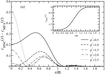
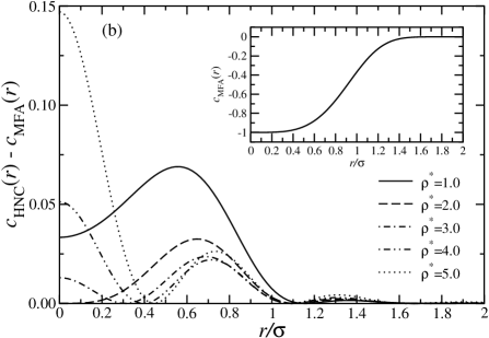
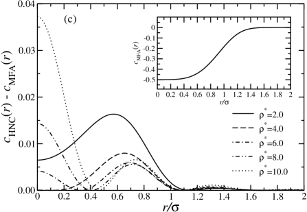
Figure 2: The main plots show the difference between the direct correlation function $c(r)$ calculated in the HNC and its MFA-approximation, $c(r)=-\beta v(r)$, for a GEM-4 model, at various densities indicated in the legends. The insets show the MFA approximation for the same quantity, which is density-independent. Each panel corresponds to a different temperature: (a) $T^{*}=0.5$; (b) $T^{*}=1.0$; (c) $T^{*}=2.0$. These are exactly the same parameter combinations as the ones for which $g(r)$ is shown in Fig. 1.

The behavior of the higher-order dcf’s is related to the density-derivative of lower-order ones through certain sum rules, to be discussed below. Hence, it is pertinent to examine the density dependence of the dcf $c(r)$ of the HNC. In Fig. 2 we show the difference between the dcf $c_{\rm HNC}(r)$ and the mean-field approximation (MFA) to the same quantity:

$$c_{\rm MFA}(r)=-\beta v(r).$$ (13)

Eq. (13) above is meaningless if the pair potential $v(r)$ diverges as $r\to 0$, because $c(r)$ has to remain finite at all $r$, as follows from exact diagrammatic expansions of the same.hansen:book In fact, the form $c(r)\sim-\beta v(r)$ denotes the large-$r$ asymptotic behavior of $c(r)$. In our case, however, where $v(r)$ lacks a hard core, the MFA-form for $c(r)$ cannot be a priori rejected on fundamental grounds; the quantity $-\beta v(r)$ remains bounded as $r\to 0$. In fact, as can be seen in Fig. 2, the deviations between the MFA and the HNC-closure are very small for $T^{*}\gtrsim 1$. In addition, the differences between $c_{\rm HNC}(r)$ and $c_{\rm MFA}(r)$ drop, both in absolute and in relative terms, as temperature grows, see the trend in Figs. 2(a)-(c). At fixed temperature, the evolution of the difference with density is nonmonotonic: it first drops as density grows and then it starts growing again at the highest densities shown in the three panels of Fig. 2.

Motivated by these findings, we employ now a second closure, namely the above-mentioned MFA, Eq. (13). Introducing the latter into the Ornstein-Zernike relation, Eq. (6), we obtain the MFA-results for the radial distribution function $g(r)$ that are also shown in Fig. 1 with dashed lines. Before proceeding to a critical comparison between the $g(r)$ obtained from the two closures, it is useful to make a clear connection between the MFA and the HNC.

As mentioned above, the members of the sequence of the $n$-th order direct correlation functions are not independent from one another; rather, they are constrained to satisfy a corresponding hierarchy of sum rules, namely:denton:pra:91 ; barrat:prl:87 ; barrat:molphys:88 ; denton:pra:89

$$\int{\rm d}^{3}r_{k}c_{0}^{(n+1)}({\bf r}_{1},\ldots,{\bf r}_{k-1},{\bf r}_{k},{\bf r}_{k+1},\ldots,{\bf r}_{n+1};\rho)=$$

$$\frac{\partial c_{0}^{(n)}({\bf r}_{1},\ldots,{\bf r}_{k-1},{\bf r}_{k+1},\ldots,{\bf r}_{n+1};\rho)}{\partial\rho}.$$ (14)

In particular, for $n=2$, we have

$$\int{\rm d}^{3}r^{\prime}c_{0}^{(3)}(r,r^{\prime},|{\bf r}-{\bf r^{\prime}}|;\rho) =$$

$$\int{\rm d}^{3}r^{\prime}c_{0}^{(3)}(r^{\prime},r,|{\bf r^{\prime}}-{\bf r}|;\rho) =$$

$$\frac{\partial c(r;\rho)}{\partial\rho},$$ (15)

where we have used the translational and rotational invariance of the fluid phase to reduce the number of arguments of the dcf’s and we show explicitly the generic dependence of $c(r)$ on $\rho$. In the MFA, one assumes $c(r)=-\beta v(r)$, with the immediate consequence

$$\frac{\partial c(r)}{\partial\rho}=0.$$ (16)

Eqs. (15) and (16) imply that the integral of $c_{0}^{(3)}$ with respect to any of its arguments must vanish for arbitrary density. As $c_{0}^{(3)}$ has a complex dependence on its arguments, this is a strong indication that $c_{0}^{(3)}$ itself vanishes. In fact, both for the Barrat-Hansen-Pastore factorization approximation for this quantitybarrat:prl:87 ; barrat:molphys:88 and for the alternative, Denton-Ashcroft $k$-space factorization of the same,denton:pra:89 the vanishing of the right-hand side of Eq. (15) implies that $c_{0}^{(3)}=0$. Now, if $c_{0}^{(3)}$ vanishes, so does also its density derivative and use of sum rule (14) for $n=3$ implies $c_{0}^{(4)}=0$. Successive use of the same for higher $n$-values leads then to the conclusion that in the MFA:

$$c_{0}^{(n)}({\bf r}_{1},{\bf r}_{2},\ldots,{\bf r}_{n};\rho)=0,\qquad(n\geq 3).$$ (17)

We can now see that the accuracy of the HNC stems from the fact that for these systems we can write

$$c(r)=-\beta v(r)+\varepsilon(r;\rho),$$ (18)

where $\varepsilon(r;\rho)$ is a small function at all densities $\rho$, offering concomitantly a very small, and the only, contribution to the quantity $\partial c(r)/\partial\rho$. This implies that $c_{0}^{(3)}$ itself is negligible by means of Eq. (15). Repeated use of Eq. (14) leads then to Eqs. (12) and shows that the contributions from the $n>2$ terms, that are ignored in the HNC, are indeed negligible. The HNC is, thus, very accurate, due to the strong mean-field character of the fluids at hand.likos:pusey The deviations between the HNC and the MFA come through the function $\varepsilon(r;\rho)$ above.

Let us now return to the discussion of the results for $g(r)$ and $c(r)$ and the relative quality of the two closures at various thermodynamic points. Referring first to Fig. 1(c), we see that at $T^{*}=2.0$ both the HNC and the MFA perform equally well. The agreement between the two (and between the MFA and MC) worsens somewhat at $T^{*}=1.0$ and even more at $T^{*}=0.5$. The MFA is, thus, an approximation valid for $T^{*}\gtrsim 1$, in agreement with previous results.criterion The reason lies in the accuracy of the low-density limit of the MFA. In general, as $\rho\to 0$, $c(r)$ tends to the Mayer function $f(r)=\exp[-\beta v(r)]-1$. If $T^{*}\gtrsim 1$, one may expand the exponential to linear order and obtain $f(r)\cong-\beta v(r)$, so that the MFA can be fulfilled.

In the HNC, it is implicitly assumed that all dcf’s with $n\geq 3$ vanish. In the MFA, this is also the case. The two closures differ in one important point, though: in the HNC, the second-order direct correlation function is not prescribed but rather determined, so that both the ‘test-particle equation’, Eq. (8), and the Ornstein-Zernike relation, Eq. (6), are fulfilled. In the MFA, it is a priori assumed that $c(r)=-\beta v(r)$, which is introduced into the Ornstein-Zernike relation and thus $h(r)$ is determined. This is one particular way of obtaining $g(r)$ in the MFA, called the Ornstein-Zernike route. Alternatively, one could follow the test-particle route in solving Eq. (8) in conjunction with Eq. (9) and the MFA-approximation, Eq. (13). In this case, the resulting expression for the total correlation function $h(r)$ in the MFA reads as

$$h(r)=\exp[-\beta v(r)-\beta\rho(h*v)(r)]-1,$$ (19)

with $*$ denoting the convolution. Previous studies with ultrasoft systems have shown that the test-particle $h(r)$ from the MFA is closer to the HNC-result than the MFA result obtained from the Ornstein-Zernike route.ingo:06 The discrepancy between the two is a measure of the approximate character of the MFA; were the theory to be exact, all routes would give the same result. As a way to quantify the approximations involved in the MFA, let us attempt to impose consistency between the test-particle and Ornstein-Zernike routes. Since $c(r)=-\beta v(r)$ in this closure, the exponent in Eq. (19) above is just the right-hand side of the Ornstein-Zernike relation, Eq. (6). Thus, if we insist that the latter is fulfilled, we obtain the constraint

$$h(r)=\exp[h(r)]-1,$$ (20)

which is strictly satisfied only for $h(r)=0$. However, as long as $|h(r)|<1$, one can linearize the exponential and an identity follows; the internal inconsistency of the MFA is of quadratic order in $h(r)$ and it follows that the MFA provides an accurate closure for the systems at hand, as long as $|h(r)|$ remains small. This explains the deviations between MFA and MC seen at small $r$ for the highest density at $T^{*}=2.0$, Fig. 1(c). The same effect can also be seen in Fig. 2(c) as a growth of the discrepancy between $c_{\rm HNC}(r)$ and $c_{\rm MFA}(r)$ at small $r$-values for the highest density shown. In absolute terms, however, this discrepancy remains very small. Note also that discrepancies at small $r$-values become strongly suppressed upon taking a Fourier transform, due to the additional geometrical $r^{2}$-factor involved in the three-dimensional integration.

It can therefore be seen that the MFA and the HNC are closely related to one another: the HNC is so successful due to the strong mean-field character of the systems under consideration. This fact has also been established and extensively discussed for the case of the Gaussian model,likos:gauss ; louis:mfa i.e., the $m=2$ member of the GEM-$m$ class. Once more, the HNC and the MFA there are very accurate for high densities and/or temperatures, where $h(r)\cong 0$ and the system’s behavior develops similarities with an ‘incompressible ideal gas’,likos:gauss in full agreement with the remarks presented above. Subsequently, the MFA and HNC closures have been also successfully applied to the study of structure and thermodynamics of binary soft mixtures.louis:mfa ; archer1 ; archer2 ; archer3 ; archer4 ; finken

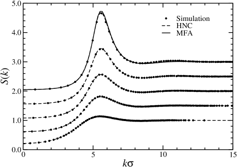
Figure 3: The structure factor $S(k)$ of the GEM-4 model at temperature $T^{*}=1.0$ and various densities, indicated below. For clarity, the curves have been shifted vertically by amounts shown in the square brackets, following the numbers that indicate the values of the density $\rho^{*}$. From bottom to top: $\rho^{*}=1.0$ [0]; $\rho^{*}=2.0$ [0.5]; $\rho^{*}=3.0$ [1.0]; $\rho^{*}=4.0$ [1.5]; $\rho^{*}=5.0$ [2.0]. The points are results from Monte Carlo simulations and the dashed lines from the HNC. As the HNC- and MFA-curves run very close to each other, we show the MFA-result by the solid curve only for the highest density, $\rho^{*}=5.0$.

A crucial difference between the Gaussian model, which belongs to the $Q^{+}$-class, and members of the $Q^{\pm}$-class, which are the subject of the present work, lies in the consequences of the MFA-closure on the structure factor $S(k)$ of the system. Since $c(r)=-\beta v(r)$, the Ornstein-Zernike relation leads to the expression

$$S(k)=\frac{1}{1+\beta\rho\tilde{v}(k)}.$$ (21)

Whereas for $Q^{+}$-potentials $S(k)$ is devoid of pronounced peaks that exceed the asymptotic value $S(k\to\infty)=1$, for $Q^{\pm}$-systems a local maximum of $S(k)$ appears at the value $k_{*}$ for which $\tilde{v}(k)$ attains its negative minimum. In Fig. 3 we show representative results for the system at hand, where it can also be seen that the HNC and the MFA yield practically indistinguishable results. In full agreement with the MC simulations, the location of the main peak of $S(k)$ is density-independent, a feature unknown for usual fluids, having its origin in the fact that $c(r)$ itself is density independent.

Associated with this is the development of a $\lambda$-line,archer4 ; finken ; stell ; ciach also known as Kirkwood instability,kirkwood:51 on which the denominator in Eq. (21) vanishes at $k_{*}$ and thus $S(k_{*})\to\infty$. The locus of points $(\rho_{\lambda},T_{\lambda})$ on the density-temperature plane for which this divergence takes place is, evidently, given by

$$\frac{T^{*}_{\lambda}}{\rho^{*}_{\lambda}}=-{\tilde{\phi}(k_{*}\sigma)}.$$ (22)

In the region $\rho\geq\rho_{\lambda}$ (equivalently: $T\leq T_{\lambda}$) on the $(\rho,T)$-plane, the MFA predicts that the fluid is absolutely unstable, since the structure factor there has multiple divergences and also develops negative parts. This holds only for $Q^{\pm}$-systems; for $Q^{+}$-ones the very same line of argumentation leads to the opposite conclusion, namely that the fluid is the phase of stability at high densities and/or temperatures. The latter conclusion has already been reached by Stillinger and coworkersstill1 ; still2 ; still3 ; still4 ; still5 in their pioneering work of the Gaussian model in the mid-1970’s, and explicitly confirmed by extensive theory and computer simulations many years later.stillinger:physica ; likos:gauss ; saija1 ; saija2 ; saija3 ; archer However, Stillinger’s original argument was based on duality relations that are strictly fulfilled only for the Gaussian model, whereas the MFA-arguments are quite general.

II.3 Nonuniform fluids

Having established the validity of the MFA for vast domains in the phase diagram of the systems under consideration as far as the uniform fluids are concerned, we now turn our attention to nonuniform ones. Apart from an obvious general interest in the properties of nonuniform fluids, the necessity to consider deviations from homogeneity in the density for $Q^{\pm}$-models is dictated by the $\lambda$-instability mentioned above: the theory of the uniform fluid contains its own breakdown, thus the system has to undergo a phase transformation to a phase with a spontaneously broken translational symmetry. Whether this transformation takes place exactly on the instability line or already at densities $\rho<\rho_{\lambda}$ (or temperatures $T>T_{\lambda}$) and which is the stable phase are some of the questions that have to be addressed. Density-functional theory of inhomogeneous systems is the appropriate theoretical tool in this direction.

Let us consider a path $\rho_{\chi}({\bf r})$ in the space of density functions, which is characterized by a single parameter $\chi$; this path starts at some reference density $\rho_{\rm r}({\bf r})$ and terminates at another density $\rho({\bf r})$. The uniqueness of the excess free energy functional and its dependence on the inhomogeneous density field $\rho({\bf r})$ allow us to integrate $\partial F_{\rm ex}[\rho]/\partial\chi$ along this path, obtaining $F_{\rm ex}[\rho]$, provided that $F_{\rm ex}[\rho_{\rm r}]$ is known. A convenient parametrization reads as $\rho_{\chi}({\bf r})=\rho_{\rm r}({\bf r})+\chi[\rho({\bf r})-\rho_{\rm r}({\bf r})]$, with $\chi=0$ corresponding to $\rho_{\rm r}({\bf r})$ and $\chi=1$ to $\rho({\bf r})$. The excess free energy of the final state can be expressed asevans:78

$$\beta F_{\rm ex}[\rho] = \beta F_{\rm ex}[\rho_{\rm r}]$$ (23)

$$- \int_{0}^{1}{\rm d}\chi\int{\rm d}^{3}rc^{(1)}({\bf r};[\rho_{\chi}])\Delta\rho({\bf r}),$$

where $c^{(1)}({\bf r};[\rho_{\chi}])$ denotes the first functional derivative of the quantity $-\beta F_{\rm ex}[\rho]$ evaluated at the inhomogeneous density $\rho_{\chi}({\bf r})$, and $\Delta\rho({\bf r})=\rho({\bf r})-\rho_{\rm r}({\bf r})$. Since $c^{(1)}({\bf r};[\rho_{\chi}])$ is in its own turn a unique functional of the density profile, repeated use of the same argument leads to a functional Taylor expansion of the excess free energy around that of a reference system, an expansion that extends to infinite order. For the particular choice of a uniform reference system, $\rho_{\rm r}({\bf r})=\rho$, we obtain then the Taylor series of Eq. (9). In general, however, the reference system does not have to have the same average density as the final one, hence the uniform density $\rho$ there must be replaced by a more general quantity $\rho_{0}$.

The usefulness of Eq. (9) in calculating the free energies of extremely nonuniform phases, such as crystals, is limited both on principal and on practical grounds. Fundamentally, there is no small parameter guiding such an expansion, since the differences between the nonuniform density of a crystal and that of a fluid are enormous; the former has extreme variations between lattice- and interstitial regions. Hence, the very convergence of the series is in doubt.singh In practice, the direct correlation functions for $n=3$ are very cumbersome to calculategerhard:00 and those for $n\geq 4$ are practically unknown.denton:pra:91 The solution is either to arbitrarily terminate the series at second orderry:79 or to seek for nonperturbative functionals.singh ; likos:prl:92 ; likos:jcp:93 ; wda1 ; wda2 ; mwda ; henderson In our case, however, things are different because, for the systems we consider, we have given evidence that the dcf’s of order $n>2$ are extremely small and we take them at this point as vanishing. Then, the functional Taylor expansion of the free energy $F_{\rm ex}[\rho]$ terminates (to the extent that the approximation holds) at second order. The Taylor series becomes a finite sum and convergence is not an issue any more.

Let us, accordingly, expand $F_{\rm ex}[\rho]$ around an arbitrary, homogeneous reference fluid of density $\rho_{0}=N_{0}/V$, taking into account that the volume $V$ is fixed but the system with density $\rho({\bf r})$ contains $N$ particles, whereas the reference fluid contains $N_{0}$ particles and, in general, $N\neq N_{0}$:

$$\beta F_{\rm ex}[\rho] = \beta F_{\rm ex}(\rho_{0})-c_{0}^{(1)}(\rho_{0})\int{\rm d}^{3}r[\rho({\bf r})-\rho_{0}]$$ (24)

$$- \frac{1}{2}\int\int{\rm d}^{3}r{\rm d}^{3}r^{\prime}c_{0}^{(2)}(|{\bf r}-{\bf r^{\prime}}|;\rho_{0})$$

$$\times [\rho({\bf r})-\rho_{0}][\rho({\bf r^{\prime}})-\rho_{0}].$$

Using $c_{0}^{(2)}(r;\rho_{0})=c_{0}^{(2)}(r)\equiv c(r)=-\beta v(r)$ and the sum rule (14) for $n=1$ together with the vanishing of the excess chemical potential at zero density, we readily obtain

$$c_{0}^{(1)}(\rho_{0})=-\beta{\tilde{v}}(0)\rho_{0}.$$ (25)

Formally substituting in Eq. (24), $\rho_{0}\to 0$ and $\rho({\bf r})\to\rho_{0}$ and making use of the fact that the excess free energy of a system vanishes with the density, we also obtain the dependence of the fluid excess free energy on the density:

$$\beta F_{\rm ex}(\rho_{0})=\frac{N_{0}}{2}\beta{\tilde{v}}(0)\rho_{0},$$ (26)

with the particle number $N_{0}$ of the reference fluid and the Fourier transform ${\tilde{v}}(k)$ of the interaction potential. Introducing Eqs. (25) and (26) into the Taylor expansion, Eq. (24) above, we obtain:

$$\beta F_{\rm ex}[\rho] = \frac{N_{0}}{2}\beta{\tilde{v}}(0)\rho_{0}$$ (27)

$$+ \beta{\tilde{v}}(0)\rho_{0}(N-N_{0})$$

$$+ \frac{\beta}{2}\int\int{\rm d}^{3}r{\rm d}^{3}r^{\prime}v(|{\bf r}-{\bf r^{\prime}}|)\rho({\bf r})\rho({\bf r^{\prime}})$$

$$- \beta\rho_{0}\int\int{\rm d}^{3}r{\rm d}^{3}r^{\prime}v(|{\bf r}-{\bf r^{\prime}}|)\rho({\bf r})$$

$$+ \frac{N_{0}}{2}\beta{\tilde{v}}(0)\rho_{0}.$$

Introducing ${\bf x}\equiv{\bf r}-{\bf r^{\prime}}$ the fourth term above becomes:

$$-\beta\rho_{0}\int{\rm d}^{3}r\,\rho({\bf r})\int{\rm d}^{3}x\,v(|{\bf x}|)=-\beta N\rho_{0}{\tilde{v}}(0).$$ (28)

Now the sum of the 1st, 2nd, 4th and 5th term in Eq. (27) yields:

$$\frac{N_{0}}{2}\beta{\tilde{v}}(0)\rho_{0}+\beta{\tilde{v}}(0)\rho_{0}(N-N_{0})$$

$$-\beta N\rho_{0}{\tilde{v}}(0)+\frac{N_{0}}{2}\beta{\tilde{v}}(0)\rho_{0}$$

$$=\beta{\tilde{v}}(0)\left[\frac{N_{0}}{2}\rho_{0}+\rho_{0}(N-N_{0})-N\rho_{0}+\frac{N_{0}}{2}\rho_{0}\right]$$

$$=\beta{\tilde{v}}(0)\left[N_{0}\rho_{0}+\rho_{0}(N-N_{0})-N\rho_{0}\right]=0.$$ (29)

This is a remarkable cancelation because then only the 3rd term in Eq. (27) survives and we obtain:

$$F_{\rm ex}[\rho]=\frac{1}{2}\int\int{\rm d}^{3}r{\rm d}^{3}r^{\prime}v(|{\bf r}-{\bf r^{\prime}}|)\rho({\bf r})\rho({\bf r^{\prime}}),$$ (30)

which is our desired result.criterion ; likos:gauss ; louis:mfa

The derivation above demonstrates that the excess free energy of any inhomogeneous phase for our ultrasoft fluids is given by Eq. (30), irrespectively of the density of the reference fluid $\rho_{0}$. This is particularly important because, usually, functional Taylor expansions are carried out around a reference fluid whose density lies close to the average density of the inhomogeneous system (crystal, in our case). However, in our systems this is impossible. The crystals occur predominantly in domains of the phase diagram in which the reference fluid is meaningless, because they are on the high density side of the $\lambda$-line. It is therefore important to be able to justify the use of the functional and to avoid the inherent contradiction of expanding around an unstable fluid. In practice, of course, the higher-order dcf’s do not exactly vanish, hence deviations from result (30) are expected to occur, in particular at low temperatures and densities. Nevertheless, the comparisons with simulations, e.g., in Refs. [criterion, ], [bianca:prl:06, ] and [archer4, ] fully justify our approximation.

A mathematical proof of the mean-field character for fluids with infinitely long-range and infinitesimally strong repulsions has existed since the late 1970’s, see Refs. [grewe1, ] and [grewe2, ]. However, even far away from fulfillment of this limit, and for conditions that are quite realistic for soft matter systems, the mean-field behavior continues to be valid.criterion ; likos:gauss ; louis:mfa The mean-field result of Eq. (30) has been put forward for the Gaussian model at high densities,likos:gauss on the basis of physical argumentation: in the absence of diverging excluded-volume interactions, at sufficiently high densities any given particle sees an ocean of others – the classical mean-field picture. The mean-field character of the Gaussian model for moderate to high temperatures was demonstrated independently in Ref. [louis:mfa, ]. Here, we have provided a more rigorous justification of its validity, based on the vanishing of high-order direct correlation functions in the fluid. It must also be noted that the mean-field approximation has recently been applied to a system with a broad shoulder and a much shorter hard-core interaction, providing good agreement with simulation resultsprimoz:07 and allowing for the formulation of a generalized clustering criterion for the inhomogeneous phases.

An astonishing similarity exists between the mean-field functional of Eq. (30) and an exact result derived for infinite-dimensional hard spheres. Indeed, for this case Frisch et al.frisch:prl:85 ; frisch:jcp:86 ; frisch:pra:87 ; frisch:pre:99 as well as Bagchi and Ricebagchi:jcp:88 have shown that

$$\beta F_{\rm ex}[\rho]=-\frac{1}{2}\int\int{\rm d}^{D}r{\rm d}^{D}r^{\prime}f(|{\bf r}-{\bf r^{\prime}}|)\rho({\bf r})\rho({\bf r^{\prime}}),$$ (31)

where $D\to\infty$ and $f(|{\bf r}-{\bf r^{\prime}}|)$ is the Mayer function of the infinite dimensional hard spheres. Again, one has a bilinear excess functional whose integration kernel does not depend on the density; in this case, this is minus the (bounded) Mayer function whereas for mean-field fluids, it is the interaction potential itself, divided by the thermal energy $k_{\rm B}T$. In fact, the Mayer function and the direct correlation function coincide for infinite-dimensional systems and higher-order contributions vanish there as well,bagchi:jcp:88 making the analogy with our three-dimensional, ultrasoft systems complete. Accordingly, infinite dimensional hard spheres have an instability at some finite $k$ at the density $\rho_{\star}$, given by $\rho_{\star}{\tilde{f}}(k)=1$. This so-called Kirkwood instabilitykirkwood:51 is of the same nature as our $\lambda$-line but hard hyperspheres are athermal, so it occurs at a single point on the density axis and not a line on the density-temperature plane. Following Kirkwood’s work,kirkwood:51 it was therefore arguedfrisch:pra:87 ; bagchi:jcp:88 that hard hyperspheres might have a second-order freezing transition at the density $\rho_{\star}$ expressed as

$$\rho_{\star}=0.239(e/8)^{D/2}\exp[z_{0}(D/2)^{1/3}]D^{1/6},$$ (32)

where the limit $D\to\infty$ must be taken and $z_{0}=1.8558$ is the value of the minimum of the Bessel function $J_{D/2}(z)$ as $D\to\infty$. Note that $\rho_{\star}\to 0$ as $D\to\infty$. Later on, Frisch and Percus argued that most likely the Kirkwood instability is never encountered because it is preempted by a first-order freezing transition.frisch:pre:99 In what follows, we will show analytically that this is also the case for our systems, which might provide a finite-dimensional realization of the above-mentioned mathematical limit.

III Analytical calculation of the freezing properties

As mentioned above, an obvious candidate for a spatially modulated phase is a periodic crystal. The purpose of this section is to employ density functional theory in order to calculate the freezing properties. Under some weak, simplifying assumptions, the problem can be solved analytically.

Adding the ideal contribution to the excess functional of Eq. (30), the free energy of any spatially modulated phase is obtained as

$$F[\rho] = F_{\rm id}[\rho]+F_{\rm ex}[\rho]$$ (33)

$$= k_{\rm B}T\int{\rm d}^{3}r\left[\ln\left[\rho({\bf r})\Lambda^{3}\right]-1\right]$$

$$+ \frac{1}{2}\int\int{\rm d}^{3}r{\rm d}^{3}r^{\prime}v(|{\bf r}-{\bf r^{\prime}}|)\rho({\bf r})\rho({\bf r^{\prime}}).$$

As we are interested in crystalline phases, we parametrize the density profile as a sum of Gaussians centered around the lattice sites $\{{\bf R}\}$, forming a Bravais lattice. In sharp contrast with systems interacting by hard, diverging potentials, however, the assumption of one particle per lattice site has to be dropped. Indeed, it will be seen that $Q^{\pm}$ systems employ the strategy of optimizing their lattice constant by adjusting the number of particles per lattice site, $n_{c}$, at any given density $\rho$ and temperature $T$. Accordingly, we normalize the profiles to $n_{c}$ and write

$$\rho({\bf r}) = n_{c}\left(\frac{\alpha}{\pi}\right)^{3/2}\sum_{{\bf R}}e^{-\alpha\left({\bf r}-{\bf R}\right)^{2}}$$ (34)

$$= \sum_{{\bf R}}\rho_{l}({\bf r}-{\bf R}),$$

where the occupation variable $n_{c}$ and the localization parameter $\alpha$ have to be determined variationally, and the lattice site density $\rho_{l}({\bf r})$ is expressed as

$$\rho_{l}({\bf r})=n_{c}\left(\frac{\alpha}{\pi}\right)^{3/2}e^{-\alpha r^{2}}.$$ (35)

Contrary to crystals of single occupancy, thus, the number of particles $N$ and the number of sites $N_{s}$ of the Bravais lattice do not coincide. In particular, it holds

$$\frac{N}{N_{s}}=n_{c},$$ (36)

and we are interested in multiple site occupancies, i.e., $n_{c}>1$ or even $n_{c}\gg 1$; it will be shown that this clustering scenario indeed minimizes the crystal’s free energy.

It is advantageous, at this point, to express the periodic density profile of Eq. (34) as a Fourier series, introducing the Fourier components $\rho_{\bf K}$ of the same:

$$\rho({\bf r})=\sum_{{\bf K}}e^{{\rm i}{\bf K}\cdot{\bf r}}\rho_{\bf K},$$ (37)

where the set $\{{\bf K}\}$ contains all reciprocal lattice vectors (RLVs) of the Bravais lattice formed by the set $\{{\bf R}\}$. Accordingly, the inverse of (37) reads as:ashcroft

$$\rho_{\bf K} = \frac{1}{v_{c}}\int_{{\mathcal{C}}}{\rm d}^{3}re^{{\rm i}{\bf K}\cdot{\bf r}}\rho({\bf r})$$ (38)

$$= \frac{1}{v_{c}}\int{\rm d}^{3}re^{{\rm i}{\bf K}\cdot{\bf r}}\rho_{l}({\bf r}),$$

where the first integral extends over the elementary unit cell ${\mathcal{C}}$ of the crystal and $v_{c}=V/N_{s}$ is the volume of ${\mathcal{C}}$, containing a single lattice site. The second integral extends over all space, where use of the periodicity of $\rho({\bf r})$ and its expression as a sum over lattice site densities, Eq. (34), has been made. Using Eq. (35) we obtain

$$\rho_{\bf K} = \frac{n_{c}}{v_{c}}e^{-K^{2}/(4\alpha)}$$ (39)

$$= \rho e^{-K^{2}/(4\alpha)}.$$

Note that the site occupancy $n_{c}$ does not appear explicitly in the functional form of the Fourier components of $\rho({\bf r})$, a feature that may seem paradoxical at first sight. However, for fixed density $\rho$ and any crystal type, the lattice constant and thus also the reciprocal lattice vectors ${\bf K}$ are affected by the possibility of clustering, thus the dependence on $n_{c}$ remains, albeit in an implicit fashion. With the density being expressed in reciprocal space, the excess free energy takes a simple form that reads as

$$\frac{F_{\rm ex}}{N}=\frac{\rho}{2}\sum_{{\bf K}}\tilde{v}(K)e^{-K^{2}/(2\alpha)}.$$ (40)

The ideal term, $F_{\rm id}[\rho]$, can also be approximated analytically, provided that the Gaussians centered at different lattice sites do not overlap. Let $a$ denote the lattice constant of any particular crystal. Then, for $\alpha a^{2}\gg 1$, the ideal free energy of the crystal takes the form

$$\frac{\beta F_{\rm id}}{N}=\ln n_{c}+\frac{3}{2}\ln\left(\frac{\alpha\sigma^{2}}{\pi}\right)-\frac{5}{2}+3\ln\left(\frac{\Lambda}{\sigma}\right),$$ (41)

where the trivial last term will be dropped in what follows, since is also appears in the expression of the free energy of the fluid and does not affect any phase boundaries. Putting together Eqs. (40) and (41), we obtain a variational free energy per particle, $\tilde{f}$, for the crystal, that reads as

$$\frac{F_{\rm id}+F_{\rm ex}}{N\epsilon} \equiv \tilde{f}(n_{c},\alpha^{*};T^{*},\rho^{*})$$ (42)

$$= T^{*}\left[\ln n_{c}+\frac{3}{2}\ln\left(\frac{\alpha^{*}}{\pi}\right)-\frac{5}{2}\right]$$

$$+ \frac{\rho^{*}}{2}\sum_{\bf Y}\tilde{\phi}(Y)e^{-Y^{2}/(2\alpha^{*})},$$

where $\alpha^{*}\equiv\alpha\sigma^{2}$ and ${\bf Y}\equiv{\bf K}\sigma$. In the list of arguments of $\tilde{f}$ the first two are variational parameters whereas the last two denote simply its dependence on temperature and density. The free energy per particle, $f_{\rm sol}(T^{*},\rho^{*})\equiv F/(N\epsilon)$ of the crystal is obtained by minimization of $\tilde{f}$, i.e.,

$$f_{\rm sol}(T^{*},\rho^{*})=\min_{\{n_{c},\alpha^{*}\}}\tilde{f}(n_{c},\alpha^{*};T^{*},\rho^{*}).$$ (43)

In carrying out the minimization, it proves useful to measure the localization length of the Gaussian profile, $\ell\equiv 1/\sqrt{\alpha}$, in units of the lattice constant $a$ instead of units of $\sigma$. To perform this change, we first express the average density $\rho$ of the crystal in terms of $n_{c}$ and $a$ as

$$\rho=\frac{zn_{c}}{a^{3}},$$ (44)

where $z$ is a lattice-dependent numerical coefficient of order unity. Introduce now the quantity $\alpha a^{2}=\gamma^{-1}$. Using Eq. (44) above, we obtain

$$\alpha^{*}=\gamma^{-1}\left(\frac{\rho^{*}}{zn_{c}}\right)^{2/3}.$$ (45)

This change of variables is just a mathematical transformation that simplifies the mathematics to follow; all results to be derived maintain their validity also in the original representation. For a further discussion of this point, see also Appendix B.

Next we make the simplifying approximation to ignore in the sum over reciprocal lattice vectors on the right-hand-side of Eq. (42) above all the RLVs beyond the first shell, whose length is $Y_{1}=K_{1}\sigma$. This is justified already because of the exponentially damping factors $\exp[-Y^{2}/(2\alpha^{*})]$ in the sum. In addition, the coefficients $|\tilde{\phi}(Y)|$ themselves decay to zero as $Y\to\infty$, with an asymptotic behavior that depends on the form of $\phi(x)$ in real space. The length of the first shell of RLVs of any Bravais lattice of lattice constant $a$ scales as $K_{1}=\zeta/a$, with some positive, lattice-dependent numerical constant $\zeta$ of order unity. Together with Eqs. (44) this implies that the length of the first RLV depends on the aggregation number $n_{c}$ as

$$Y_{1}(n_{c})=\zeta\left(\frac{\rho^{*}}{zn_{c}}\right)^{1/3},$$ (46)

and using Eq. (45), we see that the ratio $Y_{1}^{2}/(2\alpha^{*})$ takes a form that depends solely on the parameter $\gamma$, namely

$$\frac{Y_{1}^{2}(n_{c})}{2\alpha^{*}}=\frac{\gamma\zeta^{2}}{2}.$$ (47)

Introducing Eqs. (45) and (47) into (42), we obtain another functional form for the variational free energy, $\bar{f}(n_{c},\gamma;T^{*},\rho^{*})$, expressed in the new variables. It can be seen that upon making the transformation (45), the term $3/2\ln[(\alpha^{*}/\pi)]$ delivers a contribution minus $\ln n_{c}$ that exactly cancels the same term with a positive sign on the right-hand side of Eq. (42). Accordingly, the only remaining quantity of the variational free energy that still depends on $n_{c}$ is the length of the first nonvanishing RLV, $Y_{1}$, whose $n_{c}$ dependence is expressed by Eq. (46) above. Putting everything together, we obtain

$$\bar{f}(n_{c},\gamma;T^{*},\rho^{*}) = T^{*}\left[\ln\rho^{*}-1-\frac{3}{2}\left[\ln(\gamma\pi)-1\right]-\ln z\right]$$ (48)

$$+ \frac{1}{2}\rho^{*}\tilde{\phi}(0)$$

$$+ \frac{\xi_{1}\rho^{*}}{2}\tilde{\phi}\left(Y_{1}(n_{c})\right)e^{-\gamma\zeta^{2}/2},$$

where $\xi_{1}$ is the coordination number of the reciprocal lattice. Minimizing $\bar{f}$ with respect to $n_{c}$ is trivial and using Eq. (47) we obtain

$$\frac{\partial{\bar{f}}}{\partial n_{c}}=0\Rightarrow\tilde{\phi}^{\prime}(Y_{1})Y_{1}^{4}=0,$$ (49)

where the prime denotes the derivative with respect to the argument. Evidently, $Y_{1}$ coincides with $y_{*}\equiv k_{*}\sigma$, the dimensionless wavenumber for which the dimensionless Fourier transform of the interaction potential attains its negative minimum. The other mathematical solution of (49), $Y_{1}=0$, can be rejected because it yields nonpositive second derivatives or, on physical grounds, because it corresponds to a crystal with $n_{c}\to\infty$, whose occurrence would violate the thermodynamic stability of the system. Regarding second derivatives, it can be easily shown that

$$\frac{\partial^{2}\bar{f}}{\partial n_{c}^{2}}\Bigg{|}_{Y_{1}=y_{*}}>0,$$ (50)

and

$$\frac{\partial^{2}\bar{f}}{\partial\gamma\partial n_{c}}\Bigg{|}_{Y_{1}=y_{*}}=0,$$ (51)

irrespective of $\gamma$.

Having shown the coincidence of $Y_{1}$ with $y_{*}$, we set $\tilde{\phi}(Y_{1})=\tilde{\phi}(y_{*})<0$ in Eq. (48) above. Further, we notice that the term $T^{*}[\ln\rho^{*}-1]$ on the right-hand side of Eq. (48) gives the ideal free energy of a uniform fluid of density $\rho^{*}$ and the term $\rho^{*}\tilde{\phi}(0)/2$ the excess part of the same, see Eq. (26). Subtracting, thus, the total fluid free energy per particle, $f_{\rm fl}(T^{*},\rho^{*})$, we introduce the difference $\Delta{\bar{f}}\equiv\bar{f}-f_{\rm fl}$, which reads as

$$\Delta\bar{f}(n_{c}(y_{*}),\gamma;T^{*},\rho^{*})= - \frac{3T^{*}}{2}\left[\ln(\gamma\pi)+1+\frac{2\ln z}{3}\right]$$ (52)

$$+ \frac{\xi_{1}\rho^{*}}{2}\tilde{\phi}(y_{*})e^{-\gamma\zeta^{2}/2}.$$

The requirement of no overlap between Gaussians centered on different lattice sites restricts $\gamma$ to be small; a very generous upper limit is $\gamma\leq 0.05$. For such small values of $\gamma$, the first term on the right-hand side of Eq. (52) above is positive. This positivity expresses the entropic cost of localization that a crystal pays, compared to the fluid in which the delocalized particles possess translational entropy. This cost must be compensated by a gain in the excess term, which is only possible if $\tilde{\phi}(y_{*})<0$. An additional degree of freedom is offered by the candidate crystal structures. The excess free energy is minimized by the direct Bravais lattice whose reciprocal lattice has the maximum possible coordination number $\xi_{1}$. The most highly coordinated periodic arrangement of sites is fcc, for which $\xi_{1}=12$. Therefore, in the framework of this approximation, the stable lattice is bcc. It must be emphasized, though, that these results hold as long as only the first shell of RLVs is kept in the excess free energy. Inclusion of higher-order shells can, under suitable thermodynamic conditions, stabilize fcc in favor of bcc. We will return to this point later.

Choosing now $a$ as the edge-length of the conventional lattice cell of the bcc-lattice, we have $z=2$ and $\zeta=2\sqrt{2}\pi$. Evidently, the lattice constant of the crystal is density-independent, $a/\sigma=(2\sqrt{2}\pi)/y_{*}$, contrary to the case of usual crystals, for which $a\propto\rho^{-1/3}$. The density-independence of $a$ is achieved by the creation of clusters that consist of $n_{c}$ particles, each of them occupying a lattice site. The proportionality relation connecting $n_{c}$ and $\rho^{*}$ follows from Eq. (46) and reads as

$$n_{c}=\frac{8\sqrt{2}\pi^{3}}{y_{*}^{3}}\rho^{*}.$$ (53)

It remains to minimize $\bar{f}$ (equivalently, $\Delta\bar{f}$) with respect to $\gamma$ to determine the free energy of the crystal. We are interested, in particular, in estimating the ‘freezing line’, determined by the equality of free energies of the fluid and the solid.foot1 Accordingly, we search for the simultaneous solution of the equations

$$\frac{\partial{\bar{f}}}{\partial\gamma} = 0,$$ (54)

$$\Delta{\bar{f}} = 0,$$ (55)

resulting into

$$\frac{3T^{*}}{2\gamma}+\frac{\xi_{1}\zeta^{2}\rho^{*}}{4}\tilde{\phi}(y_{*})e^{-\gamma\zeta^{2}/2}=0,$$ (56)

and

$$\frac{\xi_{1}\rho^{*}}{2}\tilde{\phi}(y_{*})e^{-\gamma\zeta^{2}/2}=\frac{3T^{*}}{2}\left[\ln(\gamma\pi)+1+\frac{2\ln z}{3}\right].$$ (57)

Substituting (57) into (56) and using $z=2$ and $\zeta=2\sqrt{2}\pi$, we obtain an implicit equation for $\gamma$ that reads as

$$\gamma^{-1}=-4\pi^{2}\left[\ln\left(\gamma\pi\right)+1+\frac{2\ln 2}{3}\right],$$ (58)

and has two solutions, $\gamma_{1}\cong 0.018$ and $\gamma_{2}\cong 0.038$. Due to (50) and (51), the sign of the determinant of the Hessian matrix at the extremum is set by the sign of $\partial^{2}{\bar{f}}/\partial\gamma^{2}$; Using Eqs. (56), (57), and (58) we obtain

$$\frac{\partial^{2}{\bar{f}}}{\partial\gamma^{2}}=\frac{3T^{*}}{2\gamma}\left(\gamma^{-1}-4\pi^{2}\right),$$ (59)

which is positive for $\gamma=\gamma_{1}$ but negative for $\gamma=\gamma_{2}$. Only the first solution corresponds to a minimum and thus to freezing, whereas the second is a saddle point. Within the limits of the first-RLV-shell approximation, the crystals formed by $Q^{\pm}$-potentials feature thus a universal localization parameter at freezing: irrespective of the location on the freezing line and even of the interaction potential itself, the localization length $\ell$ at freezing is a fixed fraction of the lattice constant and the parameter $\gamma=(\alpha a^{2})^{-1}$ attains along the entire crystallization line the value

$$\gamma_{\rm f}\cong 0.018.$$ (60)

We can understand the physics behind the constancy of the ratio $\ell/a$ by examining anew the variational form of the free energy, Eq. (42). Suppose we have a fixed density $\rho^{*}$ and we vary $n_{c}$, seeking to achieve a minimum of $\tilde{f}$. An increase in $n_{c}$ implies an increase in the lattice constant $a$ by virtue of Eq. (44). The density profile takes advantage of the additional space created between neighboring sites and becomes more delocalized. This increase of the spreading of the profile brings with it an entropic gain which exactly compensates the corresponding loss from the accumulation of particles on a single site, expressed by the term $\ln n_{c}$ in Eq. (42). Expressing $\ell$ in units of $a$, i.e., working with the variable $\gamma$ instead with the original one, $\alpha^{*}$, brings the additional advantage that $\gamma_{\rm f}$ becomes independent of the pair potential. The corresponding value of $\alpha^{*}$ at freezing, $\alpha^{*}_{\rm f}$, can be obtained from Eqs. (44) and (53), and reads for the bcc-lattice as

$$\alpha^{*}_{\rm f}=\frac{y_{*}^{2}}{8\pi^{2}\gamma_{\rm f}}.$$ (61)

Here, a dependence on the pair interaction appears through the value of $y_{*}$.

Complementary to the localization parameter, we can consider the Lindemann ratio $L$ at freezing,lindemann taking into account that for the bcc lattice the nearest neighbor distance is $d=a\sqrt{3}/2$. Employing the Gaussian density parametrization, we find $\langle r^{2}\rangle=3/(2\alpha)$ and thus $L\equiv\sqrt{\langle r^{2}\rangle}/d=\sqrt{2\gamma}$. Using (60), the Lindemann ratio at freezing, $L_{\rm f}$, is determined as

$$L_{\rm f}\cong 0.189.$$ (62)

This value is considerably larger than the typical value of $0.10$ usually quoted for systems with harshly repulsive particles, such as, e.g., the bcc alcali metals and the fcc metals Al, Cu, Ag, and Au [shapiro, ], but close to the value 0.160 found by Stillinger and Weberstill3 for the Gaussian core model. The particles in the cluster crystal are quite more delocalized than the ones for singly-occupied solids. The clustering strategy enhances the stability of the crystal with respect to oscillations about the equilibrium lattice positions.

The locus of freezing points $(T^{*}_{\rm f},\rho^{*}_{\rm f})$ is easily obtained by Eqs. (57) and (58) and takes the form of of a straight line:

$$\frac{T^{*}_{\rm f}}{\rho^{*}_{\rm f}}=16\pi^{2}\gamma_{\rm f}|\tilde{\phi}(y_{*})|e^{-4\pi^{2}\gamma_{\rm f}}\cong 1.393\,|\tilde{\phi}(y_{*})|.$$ (63)

Contrary to the Lindemann ratio, which is independent of the pair potential, the freezing line does depend on the interaction potential between the particles. Yet, this dependence is a particular one, as it rests exclusively on the absolute value of the Fourier transform at the minimum, $|\tilde{\phi}(y_{*})|$ and is simply proportional to it. Comparing with the location of the $\lambda$-line from Eq. (22), $T^{*}_{\lambda}/\rho^{*}_{\lambda}=|\tilde{\phi}(y_{*})|$, we find that crystallization preempts the occurrence of the instability: indeed, at fixed $T^{*}$, $\rho^{*}_{\rm f}<\rho^{*}_{\lambda}$ or, equivalently, at fixed $\rho^{*}$, $T^{*}_{\rm f}>T^{*}_{\lambda}$; see also Fig. 4. The transition is first-order, as witnessed by the jumps of the values of $\alpha$ and $\rho_{\bf K}$ at the transition, which are nonzero for the crystal but vanish in the fluid. This is analogous to the conjectured preemption of the Kirkwood instability for infinite-dimensional hard spheres by a first-order freezing transition.frisch:pre:99

The freezing properties of $Q^{\pm}$-potentials are, thus, quite unusual and at the same time quite simple: the lattice constant is fixed due to a clustering mechanism that drives the aggregation number $n_{c}$ proportional to the density. The constant of proportionality depends solely on the wavenumber $y_{*}$ for which the Fourier transform of the pair interaction has a negative minimum, Eq. (53). The freezing line is a straight line whose slope depends only on the value of the Fourier transform of the potential at the minimum, Eq. (63). The Lindemann ratio at freezing is a universal number, independent of interaction potential and thermodynamic state.

Whereas the Lindemann ratio is employed as a measure of the propensity of a crystal to melt, the height of the peak of the structure factor of the fluid is looked upon as a measure of the tendency of the fluid to crystallize. The Hansen-Verlet criterionhv1 ; hv2 states that crystallization takes place when this quantity exceeds the value 2.85. For the systems at hand, the maximum of $S(y)$ lies at $y_{*}$, as is clear from Eq. (21). Using Eq. (63) for the location of the freezing line, we obtain the value $S_{\rm f}(y_{*})$ on the freezing line as

$$S_{\rm f}(y_{*})=\left[1+\frac{\tilde{\phi}(y_{*})}{1.393\,|\tilde{\phi}(y_{*})|}\right]^{-1}\cong 3.542.$$ (64)

This value is considerably larger than the Hansen-Verlet threshold.hv1 ; hv2 In the fluid phase, $Q^{\pm}$-systems can therefore sustain a higher degree of spatial correlation before they crystallize than particles with diverging interactions do. This property lies in the fact that some contribution to the peak height comes from correlations from within the clusters that form in the fluid; the formation of clusters already in the uniform phase is witnessed by the maxima of $g(r)$ at $r=0$ seen in Fig. 1 and also explicitly visualized in our previous simulations of the model.bianca:prl:06 These, however, do not contribute to intercluster ordering that leads to crystallization. At any rate, the Hansen-Verlet peak height is also a universal quantity for all $Q^{\pm}$ systems, in the framework of the current approximation. Moreover, both for the Lindemann and for the Hansen-Verlet criteria, the $Q^{\pm}$ systems are more robust than usual ones, since they allow for stable fluids with peak heights that exceed $2.85$ by 25% and for stable crystals with Lindemann ratios that exceed $0.10$ by almost 90%.

IV Comparison with numerical minimization

The density functional of Eq. (33) is very accurate for the bounded ultrasoft potentials at hand.criterion ; likos:gauss ; louis:mfa ; archer1 ; archer2 ; archer3 ; archer4 ; finken The modeling of the inhomogeneous density as a sum of Gaussians is an approximation but, again, an accurate one, as has been shown by comparing with simulation results,bianca:prl:06 see also section V of this work. The analytical results derived in the preceding section rest on one additional approximation, namely on ignoring the RLVs beyond the first shell. Here, we want to compare with a full minimization of the functional (33) under the modeling of the density via (34), so as to test the accuracy of the hitherto drawn conclusions on clustering and crystallization.

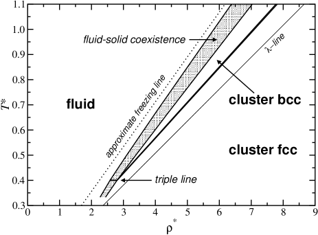
Figure 4: The phase diagram of the GEM-4 model, obtained by full minimization of the density functional (33), under the Gaussian parametrization of the density, Eq. (34), redrawn from Ref. [bianca:prl:06, ]. On the same plot, we show by the dotted line the approximate analytical result for the freezing line, Eq. (63), as well as the $\lambda$-line of the system, Eq. (22).

We work with the concrete GEM-4 system, for which the minimization of the density functional has been carried out and the phase diagram has been calculated in Ref. [bianca:prl:06, ]. In Fig. 4 we show the phase diagram obtained by the full minimization, compared with the freezing line from the analytical approximation, Eq. (63), for this system. It can be seen that the latter is a very good approximation to the full result, its quality improving slowly as the temperature grows; the analytical approximation consistently overestimates the region of stability of the crystal. Moreover, whereas the approximation only predicts a stable bcc crystal, the high-density phase of the system is fcc. Although bcc indeed is, above the triple temperature, the stable crystal immediately post-freezing, it is succeeded at higher densities by a fcc lattice, which our analytical theory fails to predict.

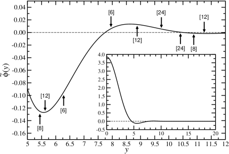
Figure 5: Inset: the Fourier transform $\tilde{\phi}(y)$ of the GEM-4 potential. Main plot: a zoom at the region of $\tilde{\phi}(y)$ in which the first few nonvanishing RLV shells of the cluster-crystals of Fig. 4 lie. The arrows denote the positions of the shells and the numbers in square brackets the numbers of distinct RLVs within each shell. These positions are the result of the full minimization of the density functional. Downwards pointing arrows pertain to the direct bcc lattice and upwards pointing arrows to the direct fcc one. In agreement with clustering predictions, the positions of the RLVs are density-independent.

All these discrepancies can be easily understood by looking at the effects of ignoring the higher RLV shells from the summation in the excess free energy, Eq. (42). Consider first exclusively the bcc lattice. In Fig. 5 we show the locations of the bcc-RLVs, as obtained from the full minimization, by the downwards pointing arrows. It can be seen that the first shell is indeed located very closely to $y_{*}$, as the analytical solution predicts. However, the next two RLV shells do have contributions and, due to their location on the hump of $\tilde{\phi}(y)$, the latter is positive. By ignoring them in performing the analytical solution, we are artificially lowering the free energy of the crystal, increasing thereby its domain of stability.

The occurrence of a fcc-lattice that beats the bcc at high densities is only slightly more complicated to understand. A first remark is that the parameter $\alpha^{*}$ increases proportionally to $\rho^{*}/T^{*}$, see the following section. Hence, the Gaussian factors from RLVs beyond the first shell, $\exp[-Y_{i}^{2}/(2\alpha^{*})]$, $i\geq 2$, gain weight in the sum as density grows. The cutoff for the RLV-sum is now provided rather by the short-range nature of $\tilde{\phi}(y)$ than by the exponential factors. Due to the increased importance of the contributions from the $i\geq 2$-terms in the excess free energy sum, the relative location of higher RLVs becomes crucial and can tip the balance in favor of fcc, although the bcc-lattice has a higher number of RLVs in its first shell than the fcc. In Fig. 5 we see that this is precisely what happens: the second RLV shell of the fcc is located fairly close to the first. In the full minimization, both of them arrange their positions so as to lie close enough to $y_{*}$. Now, a total of fourteen 1st- and 2nd-shell RLVs of the fcc can beat the twelve 1st-shell RLVs of the bcc and bring about a structural phase transformation from the latter to the former.

The relative importance of the first and second neighbors is quantified by the ratio

$$\Delta=\frac{\xi_{2}}{\xi_{1}}\frac{|\tilde{\phi}(Y_{2})|}{|\tilde{\phi}(Y_{1})|}\exp[-(Y_{2}^{2}-Y_{1}^{2})/(2\alpha^{*})],$$ (65)

where $\xi_{2}$ is the number of RLVs in the second shell. If $\tilde{\phi}(y)$ does not decay sufficiently fast to zero as $y$ grows, then the fcc lattice might even win over the bcc everywhere, since then $\Delta$ could be considerable even for values of $\alpha^{*}$ close to freezing, which are not terribly high. In fact, the penetrable sphere model (GEM-$m$ with $m\to\infty$) does not possess, on these grounds, a stable bcc phase at all.pensph:98 The prediction of the analytical theory on bcc stability has to be taken with care and is conditional to $\Delta$ being sufficiently small. A quantitative criterion on the smallness of $\Delta$ is model specific and cannot be given in general. The determination of the stable phases of the GEM-$m$ family and their dependence on $m$ can be achieved by employing genetic algorithmsdieter:jcp:05 and will be presented elsewhere.bianca:long

Notwithstanding the quantitative discrepancies between the simplified, analytically tractable version of DFT and the full one, which are small in the first place, the central conclusion of the former remains intact: the RLVs of the crystals are density-independent. Whereas the analytical approximation predicts that the length of the first RLV shell coincides with $y_{*}$, the numerical minimization brings about small deviations from this prediction. However, by reading off the relevant values from Fig. 5, we obtain $Y_{1}=5.625$ for the bcc and $Y_{1}=5.441$ for the fcc-lattice of the GEM-4 model. Comparing with the ideal value $y_{*}=5.573$, we find that the deviation between them is only a few percent. Clustering takes place, so that the lattice constants of both lattices remain fixed, a characteristic that was also explicitly confirmed by computer simulations of the model.bianca:prl:06

V Connection to harmonic theory of crystals

The use of a Gaussian parametrization for the one-particle density profiles, Eq. (34), is a standard modeling of the latter for periodic crystals. This functional form is closely related to the harmonic theory of crystals.ashcroft Each particle performs oscillations around its lattice site, experiencing thereby an effective, one-particle site potential, $V_{\rm site}({\bf s})$ that is quadratic in the displacement $s$, for small values $s/a$ [foot2, ]. Here, we will explicitly demonstrate that the Gaussian form with the localization parameter predicted from density functional theory coincides with the results obtained by performing a harmonic expansion of the said site potential.

The formation of clustered crystals is a generic property of all $Q^{\pm}$-systems, since the $\lambda$-instability is common to all of them; the form of the clusters that occupy the lattice sites, however, can be quite complex, depending on the details of the interaction. The Gaussian parametrization (34) implies that for each of the $n_{c}$ particles of the cluster, the lattice site ${\bf R}$ is an equilibrium position. In other words, the particular clusters we consider here are internally structureless. Clusters with a well-defined internal order have been found when an additional hard core of small extent is introduced.primoz:07 A necessary requirement for the lack of internal order is that the Laplacian of the interaction potential $v(r)$ be finite at $r=0$, as will be shown shortly. On these grounds, we impose from the outset on the interaction potential the additional requirement:

$$\nabla^{2}v(r)=\frac{1}{r^{2}}\left(r^{2}v^{\prime}(r)\right)^{\prime}<\infty\;\;{\rm for}\;\;r\to 0,$$ (66)

where the primes denote the derivative with respect to $r$. Eq. (66) implies that $v^{\prime}(r)$ must be at least linear in $r$ as $r\to 0$. Concomitantly, $v^{\prime\prime}(r)$ must be at least $O(1)$ as $r\to 0$. As a consequence, we have

$$v^{\prime\prime}(r)-\frac{v^{\prime}(r)}{r}\to 0\;\;{\rm for}\;\;r\to 0.$$ (67)

It can be easily checked that (67) is satisfied by all members of the GEM-$m$ class for $m>2$. It is also satisfied by the $m=2$ member, i.e., the Gaussian model, which does not display clustering because it belongs to the $Q^{+}$-class. This is, however, no contradiction. As mentioned above, the condition (67) is necessary for the formation of structureless clusters and not a sufficient one. For $Q^{\pm}$-potentials for which (67) is not fulfilled (such as the Fermi distribution models of Ref. [criterion, ]), this does not mean that clusters do not form; it rather points to the fact that they possess some degree of internal order.

The clustered crystals can be considered as Bravais lattices with a $n_{c}$-point basis. Accordingly, their phonon spectrum will feature 3 acoustic modes and $3(n_{c}-1)$ optical modes, for which the oscillation frequency $\omega(k)$ remains finite as $k\to 0$. We are interested in the case $n_{c}\gg 1$, i.e., deep in the region of stability of the crystal, where the clusters have a very high occupation number. Consequently, the phonon spectra and the particle displacements will be dominated by the optical branches. Further, we simplify the problem by choosing, in the spirit of the Einstein model of the crystal,ashcroft one specific optical phonon with $k=0$ as a representative for the whole spectrum. This mode corresponds to the relative partial displacement of two sublattices: one with $n_{c}-1$ particles on each site and one with just the remaining one particle per site. The two sublattices coincide at the equilibrium position and maintain their shape throughout the oscillation mode, consistent with the fact of an infinite-wavelength mode, $k=0$. Accordingly, the site potential felt by any one of the particles of the single-occupied sublattice, $V_{\rm site}({\bf s})$, can be expressed as

$$V_{\rm site}({\bf s})=(n_{c}-1)\left[v(s)+\sum_{{\bf R}\neq 0}v(|{\bf s}-{\bf R}|)\right],$$ (68)

where ${\bf s}$ is the relative displacement of the two sublattices. For brevity, we also define

$$W_{\rm site}({\bf s})\equiv\frac{V_{\rm site}({\bf s})}{n_{c}-1}.$$ (69)

The Taylor expansion of a scalar function $f$ around a reference point ${\bf r}$ reads as

$$f({\bf r}+{\bf s})=f({\bf r})+{\bf s}\cdot\nabla f({\bf r})+\frac{1}{2}\left({\bf s}\cdot\nabla\right)^{2}f({\bf r})+\cdots$$ (70)

Setting ${\bf r}\to 0$ and $f\to W_{\rm site}$, we obtain the quadratic expansion of the site potential; the constant $V_{\rm site}(0)$ is unimportant. For the linear term, we have

$$\nabla W_{\rm site}({\bf r}=0)=v^{\prime}(r){\bf{\hat{r}}}\Big{|}_{{\bf r}=0}+\sum_{{\bf R}\neq 0}v^{\prime}(R){\bf{\hat{R}}},$$ (71)

where ${\bf{\hat{r}}}$ and ${\bf{\hat{R}}}$ are unit vectors. The sum in (71) vanishes due to lattice inversion symmetry; the first term also, since $v^{\prime}(0)=0$. Thus, the term linear in ${\bf s}$ in the expansion of $V_{\rm site}({\bf s})$ vanishes, consistently with the fact that ${\bf s}=0$ is an equilibrium position.

We now introduce Cartesian coordinates and write ${\bf r}=(x,y,z)$, ${\bf s}=(s_{x},s_{y},s_{z})$, and ${\bf R}=(R_{x},R_{y},R_{z})$. The quadratic term in (70) takes the explicit form

$$\frac{1}{2}\left({\bf s}\cdot\nabla\right)^{2} = s_{x}s_{y}\frac{\partial^{2}}{\partial x\partial y}+s_{y}s_{z}\frac{\partial^{2}}{\partial y\partial z}+s_{z}s_{x}\frac{\partial^{2}}{\partial z\partial x}$$ (72)

$$+ \frac{1}{2}\left(s_{x}^{2}\frac{\partial^{2}}{\partial x^{2}}+s_{y}^{2}\frac{\partial^{2}}{\partial y^{2}}+s_{z}^{2}\frac{\partial^{2}}{\partial z^{2}}\right).$$

Let us consider first the mixed derivative acting on $W_{\rm site}({\bf r})$, evaluated at ${\bf r}=0$. Using Eqs. (69) and (68), we obtain

$$\frac{\partial^{2}W_{\rm site}({\bf r})}{\partial x\partial y}\Big{|}_{{\bf r}=0} = \left[\frac{xy}{r^{2}}\left(v^{\prime\prime}(r)-\frac{v^{\prime}(r)}{r}\right)\right]_{{\bf r}=0}$$ (73)

$$+ \sum_{{\bf R}\neq 0}\frac{R_{x}R_{y}}{R^{2}}\left[v^{\prime\prime}(R)-\frac{v^{\prime}(R)}{R}\right].$$

The first term on the right-hand side of (73) vanishes by virtue of (67). The second one also vanishes due to the cubic symmetry of the lattice. Clearly, the other two terms in (72) with mixed derivatives vanish as well. For the remaining terms, the cubic symmetry of the lattice implies that all three second partial derivatives of $W_{\rm site}$ at ${\bf r}=0$ are equal:

$$\frac{\partial^{2}W_{\rm site}({\bf r})}{\partial x^{2}}\Big{|}_{{\bf r}=0} = \frac{\partial^{2}W_{\rm site}({\bf r})}{\partial y^{2}}\Big{|}_{{\bf r}=0}=\frac{\partial^{2}W_{\rm site}({\bf r})}{\partial z^{2}}\Big{|}_{{\bf r}=0}$$ (74)

$$= \frac{1}{3}\nabla^{2}W_{\rm site}({\bf r})\Big{|}_{{\bf r}=0}.$$

Gathering the results, we obtain the expansion of $V_{\rm site}({\bf s})$ to quadratic order in $s$ as

$$V_{\rm site}({\bf s})=V_{\rm site}(0)+\left[\frac{(n_{c}-1)}{6}\sum_{\bf R}\nabla^{2}v(R)\right]s^{2},$$ (75)

which is isotropic in $s$, as should for a crystal of cubic symmetry. The one-particle motion is therefore harmonic; as we consider $n_{c}\gg 1$, we set $n_{c}-1\cong n_{c}$ in (75) and we obtain the effective, one-particle Hamiltonian ${\mathcal{H}}_{1}$ in the form:

$${\mathcal{H}}_{1}=\frac{p^{2}}{2m}+\kappa s^{2},$$ (76)

with

$$\kappa=\frac{n_{c}}{6}\sum_{\bf R}\nabla^{2}v(R)$$ (77)

and the momentum $p$ and mass $m$ of the particle. The density profile $\rho_{1}({\bf r})$ of this single-particle problem is easily calculated as $\langle\delta({\bf r}-{\bf s})\rangle_{{\mathcal{H}}_{1}}$, yielding

$$\rho_{1}({\bf r})=\left(\frac{\beta\kappa}{\pi}\right)^{3/2}e^{-\beta\kappa r^{2}}.$$ (78)

This is indeed a Gaussian of a single particle, with a localization parameter $\alpha_{\rm h}=\beta\kappa$; the total density on a given site will be then just $n_{c}\rho_{1}({\bf r})$, in agreement with the functional form put forward in Eq. (34).

It is useful to consider in detail the form of the localization parameter $\alpha_{\rm h}$ predicted by the harmonic theory. The parameter $\kappa$ is expressed as a sum of the values of $\psi(r)=\nabla^{2}v(r)$ over the periodic set $\{{\bf R}\}$. For every function $\psi(r)$ that possesses a Fourier transform $\tilde{\psi}(k)$, it holdsashcroft

$$\sum_{{\bf R}}\psi(R)=\rho_{s}\sum_{{\bf K}}\tilde{\psi}(K),$$ (79)

where $\{{\bf K}\}$ is the set of RLVs of $\{{\bf R}\}$ and $\rho_{s}=N_{s}/V$ is the density of lattice sites of $\{{\bf R}\}$. From (36), $\rho_{s}n_{c}=\rho$. Taking into account that the Fourier transform of $\nabla^{2}v(r)$ is $-k^{2}\tilde{v}(k)$, we obtain for the localization parameter of the harmonic theory the result

$$\alpha_{\rm h}=-\frac{\rho}{6k_{\rm B}T}\sum_{{\bf K}}K^{2}\tilde{v}(K).$$ (80)

The localization parameter must be, evidently, positive. Eq. (80) manifests the impossibility for cluster formation if the Fourier transform of the pair potential is nonnegative, i.e., for $Q^{+}$ interactions. In the preceding section, we showed within the DFT formalism that if the potential is $Q^{\pm}$, this implies the formation of cluster crystals. Harmonic theory allows us to make the opposite statement as well: if the potential is not $Q^{\pm}$, then there can be no clustered crystals. Therefore, an equivalence between the $Q^{\pm}$ character of the interaction and the formation of clustered crystals can be established. Moreover, Eq. (80) offers an additional indication as to why the RLV where $\tilde{v}(K)$ is most negative is selected as the shortest nonvanishing one by the clustered crystals: this is the best strategy in order to keep the localization parameter positive.

Harmonic theory provides, therefore, an insight into the necessity of locating the first shell of the RLVs at $k_{*}$ from a different point of view than density functional theory does. The choice $K_{1}=k_{*}$ guarantees that the particles inhabiting neighboring clusters provide the restoring forces that push any given particle back towards its equilibrium position. The density functional treatment of the preceding sections establishes that the lattice constant is chosen by $Q^{\pm}$-systems in such a way that the sum of intracluster and intercluster interactions, together with the entropic penalty for the aggregation of $n_{c}$ particles is optimized.bianca:long The unlimited growth of $n_{c}$ is avoided by the requirement of mechanical stability of the crystal. Indeed, for too high $n_{c}$-values, the lattice constant would concomitantly grow, so that the resulting restoring forces working against the thermal fluctuations, would become too weak to sustain the particles at their equilibrium positions.

Let us, finally, compare the result (80) for the localization parameter with the prediction from DFT. We consider the high-density crystal phase, for which $\alpha^{*}$ is very large, so that the simplification that only the first shell of RLVs can be kept in (42) must be dropped. Setting $\partial\tilde{f}/\partial\alpha^{*}=0$ there, we obtain

$$\frac{3T^{*}}{2\alpha^{*}}+\frac{\rho^{*}}{\left(2\alpha^{*}\right)^{2}}\sum_{{\bf Y}}Y^{2}\tilde{\phi}(Y)e^{-Y^{2}/(2\alpha^{*})}=0.$$ (81)

The function $\tilde{\phi}(y)$ is short-ranged in reciprocal space, thus the sum in (81) can be effectively truncated at some finite upper cutoff $Y_{c}$. Then, there exists a sufficiently large density $\rho^{*}$ beyond which the parameter $\alpha^{*}$ is so large that $Y^{2}/(2\alpha^{*})\ll 1$ for all $Y\leq Y_{c}$ included in the summation. Accordingly, we can approximate all exponential factors with uniti in (81), obtaining an algebraic equation for $\alpha^{*}$. Reverting back to dimensional quantities, its solution reads as

$$\alpha=-\frac{\rho}{6k_{\rm B}T}\sum_{{\bf K}}K^{2}\tilde{v}(K),$$ (82)

and is identical with the result from the harmonic theory, Eq. (80). Thus, density functional theory and harmonic theory become identical to each other at the limit of high localization. This finding completes and generalizes the result of Archer,archer who established a close relationship between the mean-field DFT and the Einstein model for the form of the variational free energy functional of the system.

Consistently with our assumptions, $\alpha$ indeed grows with density. In fact, since the set of RLVs in the sum of (82) is fixed, it can be seen that $\alpha$ is simply proportional to $\rho/T$. This peculiar feature of the class of systems we consider is not limited to the localization parameter, and its significance is discussed in the following section.

VI Connection with inverse-power potentials

As can be easily confirmed by the form of the density functional of Eq. (33), the mean-field nature of the class of ultrasoft systems considered here (both $Q^{+}$- and $Q^{\pm}$-potentials) implies that the structure and thermodynamics of the systems is fully determined by the ratio $\rho^{*}/T^{*}$ between density and temperature and not separately by $\rho^{*}$ and $T^{*}$. This is a particular type of scaling between the two relevant thermodynamic variables, reminiscent of the situation for systems interacting by means of inverse-power-law potentials $v(r)$ having the form:

$$v(r)=\epsilon\left(\frac{\sigma}{r}\right)^{n}.$$ (83)

For such systems, it can be shown that their statistical mechanics is governed by a a single coupling constant $\Gamma_{D}(n)$ expressed asweeks:prb:81

$$\Gamma_{D}(n)=\frac{\rho^{*}}{\left({T^{*}}\right)^{D/n}},$$ (84)

where $D$ is the space dimension. It would appear that inverse-powers $n=D$ satisfy precisely the same scaling as mean-field systems do but there is a condition to be fulfilled: inverse-power systems are stable against explosion, provided that $n>D$; this can be most easily seen by considering the expression for the excess internal energy per particle, $u(\rho,T)$, given byhansen:book

$$u(\rho,T)=\frac{2\pi^{D/2}\rho\epsilon\sigma^{n}}{[(D/2)-1]!}\int_{0}^{\infty}r^{D-1-n}g(r;\rho,T){\rm d}r.$$ (85)

As $g(r)\to 1$ for $r\to\infty$, we see that the integral in (85) converges only if $n>D$; a logarithmic divergence results for $n=D$. A ‘uniform neutralizing background’ has to be formally introduced for $n\leq D$, to obtain stable pseudo one-component systems, such as the one-component plasma.ocp1 ; ocp2 ; lieb Since we aim at staying with genuine one-component systems throughout, we must strictly maintain $n>D$.

Instead of taking the limit $n\to D$, we consider therefore a different procedure by setting

$$n=D+\delta$$ (86)

with some arbitrary, finite $\delta>0$. Then the coupling constant $\Gamma_{D}(n)$ becomes

$$\Gamma_{D}(D+\delta)=\rho^{*}\left(T^{*}\right)^{-\left(1+\delta/D\right)^{-1}}.$$ (87)

Now take $D\to\infty$ in this prescribed fashion, obtaining:

$$\lim_{D\to\infty}\Gamma_{D}(D+\delta)=\frac{{\rho^{*}}}{{T^{*}}},$$ (88)

which has precisely the same form as the coupling constant of our systems. In taking the limit $D\to\infty$, the exponent $n=D+\delta$ of the inverse-power potential diverges as well. It can be easily seen that in this case, the interaction $v(r)$ of Eq. (83) becomes a hard-sphere potential of diameter $\sigma$. In other words, the procedure prescribed above brings us once more to infinite-dimensional hard spheres, because also the inverse-power interaction becomes arbitrarily steep. This is a very different way of taking the limit than in Refs. [frisch:pra:87, ; frisch:pre:99, ; bagchi:jcp:88, ]: there, the interaction is hard in the first place and subsequently the limit $D\to\infty$ is taken, whereas here, interaction and dimension of space change together, in a well-prescribed fashion.

The fact that the statistical mechanics of ultrasoft fluids in three dimensions is determined by the same dimensionless parameter as that of a particular realization of hard spheres in infinite dimensions is intriguing. In a sense, ultrasoft systems are effectively high-dimensional, since they allow for extremely high densities, for which every particle interacts with an exceedingly high number of neighbors. They might, in this sense, provide for three-dimensional approximate realizations of infinite-dimensional models. This is yet another relation to infinite-dimensional systems, in addition to the one discussed at the end of Sec. II. Whether there exists a deeper mathematical connection between the two classes, remains a problem for the future.

VII Summary and concluding remarks

We have provided a detailed analysis of the properties of bounded, ultrasoft systems, with emphasis on the $Q^{\pm}$-class of interaction potentials. After having demonstrated the suppression of the contributions from the high-order direct correlation functions of the fluid phases (of order 3 and higher), we established as a consequence the accurate mean-field density functional for arbitrary inhomogeneous phases. Though this functional has been introduced and successfully used in the recent past both in staticscriterion ; bianca:prl:06 ; likos:gauss ; louis:mfa ; archer1 ; archer2 ; archer3 ; archer4 ; finken and in dynamics,rex:molphys:06 a sound justification of its basis on the properties of the uniform phase was still lacking.

The persistence of a single, finite length scale for the lattice constants of the ensuing solids of $Q^{\pm}$-systems has been understood by a detailed analysis of the structure of the free energy functional. In the fluid, the same length scale appears since the position of maximum of the liquid structure factor is independent of density. The negative minimum of the interaction potential in Fourier space sets this unique scale and forces in the crystal the formation of clusters, whose population scales proportionally with density. The analytical solution of an approximation of the density functional is checked to be accurate when confronted with the full numerical minimization of the latter. Universal Lindemann ratios and Hansen-Verlet values at crystallization are predicted to hold for all these systems, which differ substantially from those for hard matter systems. The analytical derivation of these results provides useful insight into the robustness of these structural values for an enormous variety of interactions.

Though the assumption of bounded interactions has been made throughout, recent resultsprimoz:07 indicate that both cluster formation and the persistence of the length scale survive when a short-range diverging core is superimposed on the ultrasoft potential, provided the range of the hard core does not exceed, roughly, 20% of the overall interaction range.primoz:07 The morphology of the resulting clusters is more complex, as full overlaps are explicitly forbidden; even the macroscopic phases are affected, with crystals, lamellae, inverted lamellae and ‘inverted crystals’ showing up at increasing densities. The generalization of our density functional theory to such situations and the modeling of the nontrivial, internal cluster morphology is a challenge for the future. Here, a mixed density functional, employing a hard-sphere and a mean-field part of the direct correlation function seems to be a promising way to proceed.sear ; lr1 Finally, the study of the vitrification, dynamical arrest and hopping processes in concentrated $Q^{\pm}$-systems is another problem of current interest. The recent ‘computer synthesis’ of model, amphiphilic dendrimers that do display precisely the form of $Q^{\pm}$-interactions discussed in this work,bianca:dendris offers concrete suggestions for the experimental realization of the hitherto theoretically predicted phenomena.

Appendix A Proof that the GEM-$m$ models with $m>2$ are $Q^{\pm}$-potentials

Consider the inverse Fourier transform of the spherically symmetric, bounded pair potential $v(r)$, reading as

$$v(r)=\frac{1}{2\pi^{2}}\int_{0}^{\infty}k^{2}\tilde{v}(k)\frac{\sin kr}{kr}{\rm d}k$$ (89)

From (89), it is straightforward to show that the second derivative of $v(r)$ at $r=0$ takes the form

$$v^{\prime\prime}(r=0)=-\frac{1}{6\pi^{2}}\int_{0}^{\infty}k^{4}\tilde{v}(k){\rm d}k.$$ (90)

Evidently, if $v^{\prime\prime}(r=0)\geq 0$, then $\tilde{v}(k)$ must have negative parts and hence $v(r)$ is $Q^{\pm}$. For the GEM-$m$ family, it is easy to show that $v^{\prime\prime}(r=0)=0$ for $m>2$, thus these members are indeed $Q^{\pm}$, as stated in the main text. Double-Gaussian potentials of the form

$$v(r)=|\epsilon_{1}|e^{-(r/\sigma_{1})^{2}}-|\epsilon_{2}|e^{-(r/\sigma_{2})^{2}},$$ (91)

with $|\epsilon_{1}|>|\epsilon_{2}|$, $\sigma_{1}>\sigma_{2}$, which feature a local minimum at $r=0$ are also $Q^{\pm}$, for the same reason. Notice, however, that $v^{\prime\prime}(r=0)\geq 0$ is a sufficient, not a necessary condition for membership in the $Q^{\pm}$-class. Thus, there exist $Q^{\pm}$-potentials for which $v^{\prime\prime}(r=0)<0$.

Appendix B Proof of the equivalence between the variational free energies $\tilde{f}$ and $\bar{f}$.

The introduction of the new variable $\gamma$ instead of $\alpha^{*}$, Eq. (45), and the subsequent new form $\bar{f}$ of the variational free energy, Eq. (48), are just a matter of convenience, which makes the minimization procedure more transparent. A free gift of the variable transformation is also the ensuing diagonal form of the Hessian matrix at the extremum. Fully equivalent results are obtained, of course, by working with the original variational free energy, $\tilde{f}$, Eq. (42). Here we explicitly demonstrate this equivalence.

Keeping, consistently, only the first shell of RLVs with length $Y_{1}$, $\tilde{f}$ takes the form:

$$\tilde{f}(n_{c},\alpha^{*};T^{*},\rho^{*}) = T^{*}\left[\ln n_{c}+\frac{3}{2}\ln\left(\frac{\alpha^{*}}{\pi}\right)-\frac{5}{2}\right]$$ (92)

$$+ \frac{\rho^{*}}{2}\tilde{\phi}(0)$$

$$+ \frac{\xi_{1}\rho^{*}}{2}\tilde{\phi}(Y_{1})e^{-Y_{1}^{2}/(2\alpha^{*})},$$

where $Y_{1}$ and $n_{c}$ are related via Eq. (47). Minimizations of $\tilde{f}$ with respect to $n_{c}$ and $\alpha^{*}$ yield, respectively:

$$T^{*}-\frac{\xi_{1}\rho^{*}Y_{1}}{6}\left[\frac{\partial\tilde{\phi}(Y_{1})}{\partial Y_{1}}-\frac{Y_{1}}{\alpha^{*}}\tilde{\phi}(Y_{1})\right]e^{-Y_{1}^{2}/(2\alpha^{*})}=0,$$ (93)

and

$$T^{*}+\frac{\xi_{1}\rho^{*}}{6\alpha^{*}}\tilde{\phi}(Y_{1})Y_{1}^{2}e^{-Y_{1}^{2}/(2\alpha^{*})}=0.$$ (94)

Subtracting the last two equations from one another we obtain

$$\frac{\xi_{1}\rho^{*}}{6}\tilde{\phi}^{\prime}(Y_{1})Y_{1}e^{-Y_{1}^{2}/(2\alpha^{*})}=0,$$ (95)

implying $Y_{1}=y_{*}$, as in the main text (once more, $Y_{1}=0$ is a formal solution that must be rejected on the same grounds mentioned in the text.) From this property, Eq. (53) immediately follows. Introducing $\Delta\tilde{f}\equiv\tilde{f}-f_{\rm liq}$, we can determine $\alpha^{*}_{\rm f}$ on the freezing line by requiring the simultaneous satisfaction of the minimization conditions above and of $\Delta\tilde{f}=0$. The latter equation yields

$$T^{*}\left[\ln\left(\frac{n_{c}}{\rho^{*}}\right)+\frac{3}{2}\left[\ln\left(\frac{\alpha^{*}_{\rm f}}{\pi}\right)-1\right]\right]$$

$$=-\frac{\xi_{1}\rho^{*}}{2}\tilde{\phi}(y_{*})e^{-y_{*}^{2}/(2\alpha^{*}_{\rm f})},$$ (96)

which, together with Eq. (94), yields, after some algebra

$$\ln\left[\left(\frac{\alpha^{*}_{\rm f}}{\pi}\right)\left(\frac{n_{c}}{\rho^{*}}\right)^{2/3}\right]-1=\frac{2\alpha^{*}_{\rm f}}{y_{*}^{2}}.$$ (97)

Using Eqs. (45) and (46), we obtain the equation for the $\gamma_{\rm f}$-parameter at freezing as

$$-\left[\ln\left(z^{2/3}\gamma_{\rm f}\pi\right)+1\right]=\frac{2}{\gamma_{\rm f}\zeta^{2}},$$ (98)

which, upon setting $z=2$ and $\zeta=2\sqrt{2}\pi$, yields Eq. (58) of the main text. Alternatively, we can introduce the variable $t\equiv\alpha^{*}_{\rm f}/y_{*}^{2}$ and rewrite Eq. (97) as

$$\ln\left[\left(8\sqrt{2}\right)^{2/3}\pi t\right]-1=2t,$$ (99)

which delivers $t\cong 0.704$ as a solution or, equivalently, $t=(8\pi^{2}\gamma_{\rm f})^{-1}$, in agreement with Eqs. (60) and (61) of the main text.

References

- (1) R. Sear and W. M. Gelbart, J. Chem. Phys. 110, 4582 (1999).
- (2) F. Sciortino, S. Mossa, E. Zaccarelli, and P. Tartaglia, Phys. Rev. Lett. 93, 055701 (2004).
- (3) S. Mossa, F. Sciortino, P. Tartaglia, and E. Zaccarelli, Langmuir 20, 10756 (2004).
- (4) A. I. Campbell, V. J. Anderson, J. S. van Duijneveldt, and P. Bartlett, Phys. Rev. Lett. 94, 208301 (2005).
- (5) R. Sanchez and P. Bartlett, J. Phys.: Condensed Matter 17, S3351 (2005).
- (6) A. Imperio and L. Reatto, J. Phys.: Condens. Matter 16, S3769 (2004).
- (7) A. Imperio and L. Reatto, J. Chem. Phys. 124, 164712 (2006).
- (8) C. N. Likos, C. Mayer, E. Stiakakis, and G. Petekidis, J. Phys.: Condens. Matter 17, S3363 (2005).
- (9) E. Stiakakis, G. Petekidis, D. Vlassopoulos, C. N. Likos, H. Iatrou, N. Hadjichristidis, and J. Roovers, Europhys. Lett. 72, 664 (2005).
- (10) C. N. Likos, Phys. Rep. 348, 267 (2001).
- (11) B. Krüger, L. Schäfer, and A. Baumgärtner, J. Phys. (France) 50, 319 (1989).
- (12) J. Dautenhahn and C. K. Hall, Macromolecules 27, 5399 (1994).
- (13) A. A. Louis, P. G. Bolhuis, J.-P. Hansen, and E. J. Meijer, Phys. Rev. Lett. 85, 2522 (2000).
- (14) I. O. Götze, H. M. Harreis, and C. N. Likos, J. Chem. Phys. 120, 7761 (2004).
- (15) M. Ballauff and C. N. Likos, Angew. Chemie Intl. English Ed. 43, 2998 (2004).
- (16) A. R. Denton, Phys. Rev. E 67, 011804 (2003); Erratum, ibid. 68, 049904 (2003).
- (17) D. Gottwald, C. N. Likos, G. Kahl, and H. Löwen, Phys. Rev. Lett. 92, 068301 (2004).
- (18) D. Gottwald, C. N. Likos, G. Kahl, and H. Löwen, J. Chem. Phys. 122, 074903 (2005).
- (19) C. Pierleoni, C. Addison, J.-P. Hansen, and V. Krakoviack, Phys. Rev. Lett. 96, 128302 (2006).
- (20) J.-P. Hansen and C. Pearson, Mol. Phys. 104, 3389 (2006).
- (21) A. Sütő, Phys. Rev. Lett. 95, 265501 (2005).
- (22) A. Sütő, Phys. Rev. B 74, 104117 (2006).
- (23) W. Klein, H. Gould, R. A. Ramos, I. Clejan, and A. I. Melcuk, Physica (Amsterdam) 205A, 738 (1994).
- (24) C. N. Likos, M. Watzlawek, and H. Löwen, Phys. Rev. E 58, 3135 (1998).
- (25) C. N. Likos, A. Lang, M. Watzlawek, and H. Löwen, Phys. Rev. E 63, 031206 (2001).
- (26) B. M. Mladek, D. Gottwald, G. Kahl, M. Neumann, and C. N. Likos, Phys. Rev. Lett. 96, 045701 (2006); Erratum, ibid. 97, 019901 (2006).
- (27) F. H. Stillinger and D. K. Stillinger, Physica (Amsterdam) 244A, 358 (1997).
- (28) A. Lang, C. N. Likos, M. Watzlawek, and H. Löwen, J. Phys.: Condens. Matter 12, 5087 (2000).
- (29) S. Prestipino, F. Saija, and P. V. Giaquinta, Phys. Rev. E 71, 050102 (2005),
- (30) F. Saija and P. V. Giaquinta, Chem. Phys. Chem. 6, 1768 (2005)
- (31) S. Prestipino, F. Saija, and P. V. Giaquinta, J. Chem. Phys. 123, 144110 (2005).
- (32) A. J. Archer, Phys. Rev. E 72, 051501 (2006).
- (33) D. Frenkel, Nature (London) 440, 4-5 (02 March 2006).
- (34) See the extensive commentary by D. Frenkel in: Journal Club for Condensed Matter Physics, selection of March 2006, link http://www.bell-labs.com/jc-cond-mat/march/march_2006.html.
- (35) M. A. Glaser, G. M. Grason, R. D. Kamien, A. Košmrlj, C. D. Santagelo, and P. Ziherl, preprint, cond-mat/0609570.
- (36) D. Ruelle, Statistical Mechanics (Benjamin, New York, 1969).
- (37) M.-J. Fernaud, E. Lomba, and L. L. Lee, J. Chem. Phys. 112, 810 (2000).
- (38) J.-P. Hansen and I. R. McDonald, Theory of Simple Liquids, 3rd ed. (Elsevier, Amsterdam, 2006).
- (39) J. K. Percus, Phys. Rev. Lett. 8, 462 (1962).
- (40) J. K. Percus, in The Equilibrium Theory of Classical Fluids, edited by H. L. Fritsch and J. L. Lebowitz (Benjamin, New York, 1964).
- (41) A. R. Denton and N. W. Aschroft, Phys. Rev. A 44, 1219 (1991).
- (42) A. Yethiraj, H. Fynewever, and C.-Y. Shew, J. Chem. Phys. 114, 4323 (2001).
- (43) Y. Singh, Phys. Rep. 207, 351 (1991).
- (44) R. Evans, Adv. Phys. 28, 143 (1979).
- (45) T. V. Ramakrishnan and M. Yussouff, Phys. Rev. B 19, 2775 (1979).
- (46) A. D. J. Haymet and D. W. Oxtoby, J. Chem. Phys. 74, 2559 (1981).
- (47) A. R. Denton and N. W. Ashcroft, Phys. Rev. A 41, 2224 (1990).
- (48) M. Baus and J.-P. Hansen, Phys. Rep. 59, 1 (1980).
- (49) S. Ichimaru, H. Iyetomi, and S. Tanaka, Phys. Rep. 149, 91 (1987).
- (50) J.-L. Barrat, J.-P. Hansen, and G. Pastore, Phys. Rev. Lett. 58, 2075 (1987).
- (51) J.-L. Barrat, J.-P. Hansen, and G. Pastore, Mol. Phys. 63, 747 (1988).
- (52) A. R. Denton and N. W. Ashcroft, Phys. Rev. A 39, 426 (1989).
- (53) C. N. Likos, N. Hoffmann, H. Löwen, and A. A. Louis, J. Phys.: Condens. Matter 14, 7681 (2002).
- (54) I. O. Götze, A. J. Archer, and C. N. Likos, J. Chem. Phys. 124, 084901 (2006).
- (55) A. A. Louis, P. G. Bolhuis, and J.-P. Hansen, Phys. Rev. E 62, 7961 (2000).
- (56) A. J. Archer and R. Evans, Phys. Rev. E 64, 041501 (2001).
- (57) A. J. Archer and R. Evans, J. Phys.: Condens. Matter 14, 1131 (2002).
- (58) A. J. Archer, C. N. Likos, and R. Evans, J. Phys.: Condens. Matter 14, 12031 (2002).
- (59) A. J. Archer, C. N. Likos, and R. Evans, J. Phys.: Condens. Matter 16, L297 (2004).
- (60) R. Finken, J.-P. Hansen, and A. A. Louis, J. Phys. A 37, 577 (2004).
- (61) G. Stell, J. Stat. Phys. 78, 197 (1995).
- (62) A. Ciach, W. T. Góźdź, and R. Evans, J. Chem. Phys. 118, 9726 (2003).
- (63) J. G. Kirkwood, in Phase Transitions in Solids, ed. by R. Smoluchowski, J. E. Meyer, and A. Weyl (Wiley, New York, 1951).
- (64) F. H. Stillinger, J. Chem. Phys. 65, 3968 (1976).
- (65) F. H. Stillinger and T. A. Weber, J. Chem. Phys. 68, 3837 (1978).
- (66) F. H. Stillinger and T. A. Weber, Phys. Rev. B 22, 3790 (1980).
- (67) F. H. Stillinger, J. Chem. Phys. 70, 4067 (1979).
- (68) F. H. Stillinger, Phys. Rev. B 20, 299 (1979).
- (69) S. Jorge, G. Kahl, E. Lomba, and J. L. F. Abascal, J. Chem. Phys. 113, 3302 (2000).
- (70) C. N. Likos and N. W. Ashcroft, Phys. Rev. Lett. 69, 316 (1992); Erratum, ibid., 69, 3134 (1992).
- (71) C. N. Likos and N. W. Ashcroft, J. Chem. Phys. 99, 9090 (1993).
- (72) W. A. Curtin and N. W. Ashcroft, Phys. Rev. A 32, 2909 (1985).
- (73) W. A. Curtin and N. W. Ashcroft, Phys. Rev. Lett. 56, 2775 (1986); Erratum, ibid., 57, 1192 (1986).
- (74) A. R. Denton and N. W. Ashcroft, Phys. Rev. A 39, 4701 (1989).
- (75) R. Evans, in Fundamentals of Inhomogeneous Fluids, ed. by D. Henderson (Marcel Dekker, New York 1992).
- (76) N. Grewe and W. Klein, J. Math. Phys. 18, 1729 (1977).
- (77) N. Grewe and W. Klein, J. Math. Phys. 18, 1735 (1977).
- (78) H. L. Frisch, N. Rivier, and D. Wyler, Phys. Rev. Lett. 54, 2061 (1985).
- (79) W. Klein and H. L. Frisch, J. Chem. Phys. 84, 968 (1986).
- (80) H. L. Frisch and J. K. Percus, Phys. Rev. A 35, 4696 (1987).
- (81) H. L. Frisch and J. K. Percus, Phys. Rev. E 60, 2942 (1999).
- (82) B. Bagchi and S. A. Rice, J. Chem. Phys. 88, 1177 (1987).
- (83) N. W. Ashcroft and N. D. Mermin, Solid State Physics (Holt Saunders, Philadelphia, 1976).
- (84) Strictly speaking, there is no freezing line on the density-temperature plane but rather a domain of coexistence, since it is equality of the grand potentials that determines phase coexistence. Nevertheless, the condition of equality of the Helmholtz free energies determines a line that runs between the melting- and crystallization lines and therefore serves as a reliable locator of the freezing transition.
- (85) F. A. Lindemann, Phys. Z. 11, 609 (1910).
- (86) J. N. Shapiro, Phys. Rev. B 1, 3982 (1970).
- (87) J.-P. Hansen and L. Verlet, Phys. Rev. 184, 151 (1969).
- (88) J.-P. Hansen and D. Schiff, Mol. Phys. 25, 1281 (1973).
- (89) D. Gottwald, G. Kahl, and C. N. Likos, J. Chem. Phys. 122, 204503 (2005).
- (90) B. M. Mladek, D. Gottwald, G. Kahl, M. Neumann, and C. N. Likos, in preparation (2007).
- (91) A very important exception is the hard-sphere potential, for which no harmonic expansion can be made. The fact that hard-sphere crystals do still have density profiles that are very well modeled by Gaussians, calls for a different explanation there. It can be argued that the huge number of uncorrelated collisions with the neighbors, together with the central limit theorem, are responsible for the Gaussianity of density profiles in hard-sphere solids.
- (92) J. D. Weeks, Phys. Rev. B 24, 1530 (1981).
- (93) E. Lieb, Rev. Mod. Phys. 48, 553 (1976).
- (94) M. Rex, C. N. Likos, H. Löwen, and J. Dzubiella, Mol. Phys. 104, 527 (2006) and references therein.
- (95) B. M. Mladek, G. Kahl, and C. N. Likos, in preparation (2007).