Enhancing the Conductance of a Two-Electron Nanomechanical Oscillator

Abstract

We consider electron transport through a mobile island (i.e., a nanomechanical oscillator) which can accommodate one or two excess electrons and show that, in contrast to immobile islands, the Coulomb blockade peaks, associated with the first and second electrons entering the island, have different functional dependence on the nano-oscillator parameters when the island coupling to its leads is asymmetric. In particular, the conductance for the second electron (i.e., when the island is already charged) is greatly enhanced in comparison to the conductance of the first electron in the presence of an external electric field. We also analyze the temperature dependence of the two conduction peaks and show that these exhibit different functional behaviors.

I Introduction

Electron transport in nanoelectromechanical systems (NEMS), such as suspended nano-beams, cantilevers, and nano-oscillators, is now attracting considerable attention reviews . In shuttles, electrons can be carried by a single nano-particle or single molecule, which oscillates between two leads. This mechanical motion strongly modifies the lead-shuttle tunneling matrix elements, affecting the charge transfer. Theoretical theory ; McC1 ; DMLmech and experimental Park1 ; exp studies of nanooscillators clearly demonstrated the influence of mechanical motion on their electrical properties.

Previously, electron transport through a moving island was examined in the strong Coulomb-blockade regime, when the conducting level of the nano-oscillator can only be single populated, with higher-energy states being energetically inaccessible. Here, we demonstrate that a charged island behaves differently from an uncharged one; correspondingly, the possible double occupation of the conducting level leads to a situation where the Coulomb blockade peaks, associated with the first and second electrons transferred through the island, have different dependencies on the nano-oscillator parameters. Moreover, we show that the double occupation leads to a conductance enhancement for the second electron entering the island. To achieve that, we apply a previously-developed approach Smirnov1 ; Smirnov2 which makes it possible to examine the case of finite on-site Coulomb interaction.

It should be noted that the moving island studied in this work can be considered as a shuttle because of its actual function: shuttling. When the island moves closer to the left lead, increasing that matrix element, it loads an electron. Then, the island moves closer to the right lead and unloads the electron. Therefore, this describes the operation of an electron shuttle. We have opted to use the term “mobile island” for this “electron shuttle” because in the nanomechanical community oscillators exhibiting an instability are called “shuttles”. Still, functionally, the moving island described here is effectively a shuttle.

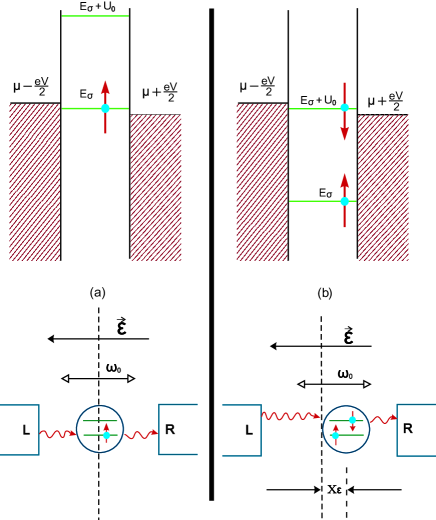
Figure 1: (Color online) Schematic diagram of electron transport through (a) uncharged and (b) charged nano-oscillator (electron charge e is negative).

Usually, a nano-oscillator is considered to be placed symmetrically between the leads. However, recently several works discussed the situation when there is an asymmetry in the lead-oscillator coupling produced either by the difference in the tunnel matrix elements Flensberg ; Fazio or by the spatial shift of the equilibrium oscillator position Milburn1 . In the latter case, it was theoretically proposed that, if the island is closer to one lead than to the other, the current through the structure depends exponentially on this spatial shift (with the tunnelling length $\lambda$), because the overlap integral of the electron wave functions in the island and in the leads, involved in the tunnel matrix elements, exponentially decreases with distance. In the model of Ref. Milburn1 , this small displacement, shifting the island close to one of the leads, was produced by the large magnetic field gradient acting on the spin of the nitrogen or phosphorus impurity incorporated into their model of a $C_{60}$ shuttle. Here we show that such displacement can be achieved naturally in the island without impurities with an excess electron in an electric field produced by the source-drain voltage or an external capacitor (see Fig. 1). Moreover, this kind of spatial asymmetry can be associated with the Jahn-Teller effect: when an orbital state of an ion is degenerate for symmetry reasons, the ligands will experience forces driving the system to a lower-symmetry configuration, lowering its energy. Consequently, the ligand position between the two ions is not symmetric and changes with the electron transfer from one ion to the other. Oscillations of such ligands, either as oxygen atoms in manganites Satpathy or rare-earth atoms in filled skutterudites Hotta , were analyzed jointly with the Jahn-Teller effect. However, the tunnelling length was assumed to be infinite in Refs. Satpathy ; Hotta and the dependence of the tunnel matrix elements on the oscillator position was not taken into account. Here we consider these effects and find a remarkably rich behavior of the conductance of nano-oscillators, if the matrix elements have an asymmetry as in Refs. Flensberg ; Fazio .

The present paper is organized as follows. Section II introduces the pertinent Hamiltonian including all interactions. The equations of motion for the electron creation/annihilation operators are derived in Sec. III. The equations for the electron populations and the populations correlator are derived and solved in Sec. IV. In Sec. V we obtain explicit expressions for the lead-to-lead current and discuss the dependence of the conductance on the system parameters. The conclusions of this work are presented in Sec. VII.

II Formulation

To examine electron transport through a moving island, we assume that the island has a single spatial state which can be populated by two electrons having opposing spin projections, $\sigma$ and $\bar{\sigma}$, with finite on-site Coulomb interaction ($U_{0}\neq\infty$). It should be noted that here we consider the situation where the coupling of the nano-oscillator to the leads is weak, so the Kondo-like correlations are not important. The Hamiltonian of this system is given by ($\alpha=L,R$ for left, right; $\sigma=1,2$ for spin up, down; $\bar{\sigma}=2,1$ )

$$H=\sum_{\sigma}E_{\sigma}a_{\sigma}^{+}a_{\sigma}+U_{0}a_{\sigma}^{+}\,a_{\sigma}\,a_{\bar{\sigma}}^{+}\,a_{\bar{\sigma}}+\sum_{k\alpha\sigma}E_{k\alpha\sigma}\,c_{k\alpha\sigma}^{+}\,c_{k\alpha\sigma}+H_{{\rm osc}}+H_{{\rm tun}},$$ (1)

where $a^{+}_{\sigma}$ ($a_{\sigma}$) are the creation (annihilation) operators for the electrons in the island and $c^{+}_{k\alpha\sigma}$ ($c_{k\alpha\sigma}$) are the creation (annihilation) operators with wavevector $k$ in the $\alpha$-lead. The tunneling term,

$$H_{{\rm tun}}=-\sum_{k\alpha\sigma}T_{k\alpha}\,w_{\alpha}(x)\,c_{k\alpha\sigma}^{+}\,a_{\sigma}\,+H.\,c.,$$ (2)

has tunneling amplitudes depending explicitly on the position $x$ of the island as

$$w_{\alpha}(x)=\exp\left(\frac{x}{\lambda_{\alpha}}\right)$$

with the tunneling lengths $\lambda_{L}=-\lambda$ and $\lambda_{R}=\lambda$ for the left and right leads, respectively. The Hamiltonian of the nanomechanical oscillator also contains the interaction between the charge stored in the oscillator and an effective electric field $\cal{E}$, as

$$H_{{\rm osc}}={p^{2}\over 2M}+{M\omega_{0}^{2}\,x^{2}\over 2}-e\,{\cal E}x\sum_{\sigma}N_{\sigma}.$$ (3)

This field ${\cal E}$ can be produced by the voltage applied to the leads, by the Jahn-Teller effect, or even by an independently controlled electric field, if the structure is placed inside an external capacitor. Here, $N_{\sigma}=a_{\sigma}^{+}\,a_{\sigma}$ is the electron population operator, and $M$ and $\omega_{0}$ are the effective mass and the resonant frequency of the nano-oscillator, respectively.

After the unitary transformation $U=\exp\left\{-ip\,\sum_{\sigma}x_{\cal{E}}\,N_{\sigma}\right\}$, where $x_{\cal{E}}=e\cal{E}$/$(M\omega_{0}^{2})$, we obtain the usual expression for the oscillator Hamiltonian, $H_{{\rm osc}}=p^{2}/2M+M\omega_{0}^{2}x^{2}/2$, and the modified electron operators,

$$a_{\sigma}^{\prime}=U^{+}a_{\sigma}U=e^{-ipx_{\sigma}}a_{\sigma},$$ (4)

and tunnel matrix elements,

$$w_{\alpha}^{\prime}(x)=w_{\alpha}(x+\sum_{\sigma^{\prime}}x_{\cal{E}}N_{\sigma^{\prime}}).$$ (5)

Using the properties of Fermi operators ($N_{\sigma}^{2}=N_{\sigma},\ a_{\sigma}N_{\sigma}=a_{\sigma},\ N_{\sigma}a_{\sigma}=0,\ ...$), we obtain

$$w_{\alpha}(x+x_{\cal{E}}(N_{\sigma}+N_{\bar{\sigma}})) = w_{\alpha\sigma}(x)+[w_{\alpha}(x+x_{\cal{E}})-w_{\alpha}(x)]N_{\sigma}$$

$$+[w_{\alpha}(x+x_{\cal{E}})-w_{\alpha}(x)]N_{\bar{\sigma}} + [w_{\alpha}(x+2x_{\cal{E}})-2w_{\alpha}(x+x_{\cal{E}})+w_{\alpha}(x)]N_{\sigma}N_{\bar{\sigma}},$$ (6)

and

$$a_{\sigma}w_{\alpha}(x+x_{\cal{E}}(N_{\sigma}+N_{\bar{\sigma}}))=a_{\sigma}w_{\alpha}(x+x_{\cal{E}})+A_{\sigma}[w_{\alpha}(x+2x_{\cal{E}})-w_{\alpha}(x+x_{\cal{E}})].$$ (7)

Here, we have introduced the Fermi operator $A_{\sigma}=N_{\bar{\sigma}}a_{\sigma}$. Accordingly, the tunneling term has a form

$$H_{{\rm tun}}=-\sum_{k\alpha\sigma}T_{k\alpha}\,c_{k\alpha\sigma}^{+}\,B_{\alpha\sigma}-H.\,c.,$$ (8)

where $B_{\alpha\sigma}$ is the Fermi operator given by

$$B_{\alpha\sigma}=a_{\sigma}(u_{\alpha}+v_{\alpha}\,N_{\bar{\sigma}}),$$ (9)

with the first term responsible for the electron tunneling from the unoccupied island and the second one describing the electron transfer through the double-populated level. Here,

$$u_{\alpha}=u_{\alpha}^{mn}\,\rho_{mn}\ \ \ {\rm and}\ \ \ v_{\alpha}=v_{\alpha}^{mn}\,\rho_{mn},$$ (10)

where

$$\rho_{mn}=|m\rangle\langle n|\ \ \ (m,n=0,1,..)$$ (11)

are the eigenstates of the mechanical oscillator Hamiltonian, and the matrix elements of the tunneling amplitudes are given by

$$u_{\alpha}^{mn}=\langle m|\ \exp\left(\frac{x}{\lambda_{\alpha}}\right)\exp(-ipx_{\cal{E}})\ |n\rangle$$ (12)

and

$$v_{\alpha}^{mn}=u_{\alpha}^{mn}\,\left[\exp\left(\frac{x}{\lambda_{\alpha}}\right)-1\right].$$ (13)

Equations (12,13) can be considered as a generalization of the Frank-Condon factors FC accounting for the overlap integral of the vibrational states before and after the transition. It is evident that the Frank-Condon factors are different for the first and second electrons entering the island because the center of the oscillations is shifted in the case of the charged island (see Fig. 1). It should be emphasized that by introducing the operators $B_{\alpha\sigma}$ we are able to derive the equations of motion analytically, without the use of the Hartree-Fock approximation, assuming only a weak  lead-island tunnelling coupling. From a general point of view, the method presented here is equivalent to the master equation approach.

III Equations of Motion

Equations of motion for the island electron operators obtained from the Hamiltonian, Eq. (1) are given by

$$i\dot{a}_{\sigma}=E_{\sigma}a_{\sigma}+U_{0}A_{\sigma}-\sum_{k\alpha\sigma}T_{k\alpha\sigma}^{*}(u_{\alpha\sigma}^{+}+v_{\alpha\sigma}^{+}N_{\bar{\sigma}})c_{k\alpha\sigma}+$$

$$\sum_{k\alpha\sigma}T_{k\alpha\bar{\sigma}}c_{k\alpha\bar{\sigma}}^{+}a_{\sigma}a_{\bar{\sigma}}v_{\alpha\bar{\sigma}}+\sum_{k\alpha\sigma}T_{k\alpha\bar{\sigma}}^{*}v_{\alpha\sigma}^{+}a_{\bar{\sigma}}^{+}a_{\sigma}c_{k\alpha\bar{\sigma}}$$ (14)

and

$$i\dot{A}_{\sigma}=(E_{\sigma}+U_{0})a_{\sigma}-\sum_{k\alpha\sigma}T_{k\alpha\sigma}^{*}(u_{\alpha\sigma}^{+}+v_{\alpha\sigma}^{+})N_{\bar{\sigma}}c_{k\alpha\sigma}+$$

$$\sum_{k\alpha\sigma}T_{k\alpha\bar{\sigma}}c_{k\alpha\bar{\sigma}}^{+}a_{\bar{\sigma}}a_{\sigma}u_{\alpha\bar{\sigma}}+\sum_{k\alpha\sigma}T_{k\alpha\bar{\sigma}}^{*}(u_{\alpha\bar{\sigma}}^{+}+v_{\alpha\bar{\sigma}}^{+})a_{\bar{\sigma}}^{+}a_{\sigma}c_{k\alpha\bar{\sigma}}.$$ (15)

Accordingly, equations for the ensemble averaged  island populations can be written as

$$\frac{d\langle N_{\sigma}\rangle}{dt}=-i\sum_{k\alpha\sigma}T_{k\alpha\sigma}\langle c_{k\alpha\sigma}^{+}B_{\alpha\sigma}\rangle+H.\,c.$$ (16)

and

$$\frac{d\langle{N}_{\sigma}N_{\bar{\sigma}}\rangle}{dt}=-i\sum_{k\alpha\sigma}T_{k\alpha\sigma}\langle c_{k\alpha\sigma}^{+}A_{\alpha\sigma}\rangle(\langle u_{\alpha\sigma}\rangle+\langle v_{\alpha\sigma}\rangle)-i\sum_{k\alpha\sigma}T_{k\alpha\bar{\sigma}}\langle c_{k\alpha\bar{\sigma}}^{+}A_{\alpha\bar{\sigma}}\rangle(\langle u_{\alpha\bar{\sigma}}\rangle+\langle v_{\alpha\bar{\sigma}}\rangle)+H.\,c.$$ (17)

The equation of motion for the electron operators in the leads are given by

$$i\dot{c}_{k\alpha\sigma}=E_{k\alpha\sigma}c_{k\alpha\sigma}-T_{k\alpha\sigma}B_{\alpha\sigma}.$$ (18)

In the case of weak lead-island tunnel coupling, the solution of this equation can be represented as

$$c_{k\alpha\sigma}(t)=c_{k\alpha\sigma}^{(0)}(t)-T_{k\alpha\sigma}\int dt_{1}\;g_{k\alpha\sigma}^{r}(t,t_{1})\;B_{\alpha\sigma}(t_{1}),$$ (19)

where $c_{k\alpha\sigma}^{(0)}(t)$ is the unperturbed electron operator and $g_{k\alpha\sigma}^{r}(t,t_{1})$ is the retarded Green function of the electrons in the leads, given by

$$g_{k\alpha\sigma}^{r}(t,t_{1})=-i\langle[c_{k\alpha\sigma}^{(0)}(t),c_{k\alpha\sigma}^{(0)+}(t_{1})]_{+}\rangle\theta(t-t_{1})=-ie^{-iE_{k\alpha\sigma}(\tau)}\theta(\tau),$$ (20)

where $[...,...]_{+}$ is the anticommutator, $\tau=t-t_{1}$, and $\theta(\tau)$ is the unit step function. It should be emphasized that the non-Markovian dynamics involved in Eq. (19) allows us to reveal manifestations of the oscillatory mechanical motion during the tunneling events.

IV Electron populations and populations correlator

IV.1 Free-evolution approximation

To determine electron populations in the island and the correlator of the populations having different spin projections, we substitute Eq. (19) into Eqs. (16,17). The correlators of the type $\langle c_{k\alpha\sigma}^{(0)+}(t)B_{\alpha\sigma}(t)\rangle$ can be rewritten using the formula

$$\sum_{k\alpha\sigma}T_{k\alpha\sigma}\langle c_{k\alpha\sigma}^{(0)+}(t)B_{\alpha\sigma}(t)\rangle=-\sum_{k\alpha\sigma}|T_{k\alpha\sigma}|^{2}\int^{t}_{-\infty}dt_{1}\langle c_{k\alpha\sigma}^{(0)+}(t)c_{k\alpha\sigma}^{(0)}(t_{1})\rangle\langle[B_{\alpha\sigma}(t),B^{+}_{\alpha\sigma}(t_{1})]_{+}\rangle.$$ (21)

To decouple the correlators for the electron operators in the island, we use the approximation of their free evolution, which is valid in the case of weak lead-island tunneling. The free evolutions of the operators $a_{\sigma},A_{\sigma},$ and $B_{\alpha\sigma}$ are given by

$$a_{\sigma}(t)=e^{-iE_{\sigma}\tau}[a_{\sigma}(t_{1})-(1-e^{-iU_{0}\tau})A_{\sigma}(t_{1})],$$ (22)

$$A_{\sigma}(t)=e^{-i(E_{\sigma}+U_{0})\tau}A_{\sigma}(t_{1}),$$ (23)

and

$$B_{\alpha\sigma}(t)=e^{-iE_{\sigma}\tau}[a_{\sigma}(t_{1})-A_{\sigma}(t_{1})]u_{\alpha\sigma}(t)+e^{-i(E_{\sigma}+U_{0})\tau}A_{\sigma}(t_{1})(u_{\alpha\sigma}+v_{\alpha\sigma})(t).$$ (24)

Accordingly,

$$\langle B_{\alpha\sigma}(t)B_{\alpha\sigma}^{+}(t_{1})\rangle=e^{-iE_{\sigma}\tau}\langle u_{\alpha\sigma}(t)u_{\alpha\sigma}^{+}(t_{1})\rangle\langle 1-N_{\sigma}-N_{\bar{\sigma}}+N_{\sigma}N_{\bar{\sigma}}\rangle+$$

$$e^{-i(E_{\sigma}+U_{0})\tau}\langle(u_{\alpha\sigma}(t)+v_{\alpha\sigma}(t))(u_{\alpha\sigma}^{+}(t_{1})+v_{\alpha\sigma}^{+}(t_{1}))\rangle\langle N_{\bar{\sigma}}-N_{\sigma}N_{\bar{\sigma}}\rangle,$$ (25)

and

$$\langle B_{\alpha\sigma}^{+}(t_{1})B_{\alpha\sigma}(t)\rangle=e^{-iE_{\sigma}\tau}\langle u_{\alpha\sigma}^{+}(t_{1})u_{\alpha\sigma}(t)\rangle\langle N_{\sigma}-N_{\sigma}N_{\bar{\sigma}}\rangle+$$

$$e^{-i(E_{\sigma}+U_{0})\tau}\langle(u_{\alpha\sigma}^{+}(t_{1})+v_{\alpha\sigma}^{+}(t_{1}))(u_{\alpha\sigma}(t)+v_{\alpha\sigma}(t))\rangle\langle N_{\sigma}N_{\bar{\sigma}}\rangle.$$ (26)

The free-evolution approximation can also be used to calculate the correlators of the mechanical operators. Using $\rho_{mn}(t)=e^{i\omega_{mn}(t-t_{1})}\rho_{mn}(t_{1})$, we obtain:

$$\langle u_{\alpha\sigma}(t)u_{\alpha\sigma}^{+}(t_{1})\rangle=\sum_{mn}|u_{\alpha\sigma}^{mn}|^{2}e^{i\omega_{mn}\tau}\langle\rho_{m}\rangle,$$

$$\langle u_{\alpha\sigma}^{+}(t)u_{\alpha\sigma}(t_{1})\rangle=\sum_{mn}|u_{\alpha\sigma}^{mn}|^{2}e^{-i\omega_{mn}\tau}\langle\rho_{n}\rangle,$$ (27)

where $\langle\rho_{n}\rangle=\langle\rho_{nn}\rangle$ is the steady-state distribution of the mechanical degrees of freedom and $\omega_{mn}=\epsilon_{m}-\epsilon_{n}=\omega_{0}(m-n)$.

IV.2 Electron occupations

In the absence of an external magnetic field, the averaged electron populations, $\langle N_{1}\rangle$ and $\langle N_{2}\rangle$, should be equal: $\langle N_{1}\rangle=\langle N_{2}\rangle=\langle N\rangle.$ As a result, we obtain the following equations for the averaged electron occupation $\langle N\rangle$ and for the correlation function of the populations with opposite spin projections, $\langle N_{1}N_{2}\rangle$,

$$\eta_{1}\langle N_{1}N_{2}\rangle=\eta_{2}\langle N\rangle,\ \ \eta_{3}\langle N\rangle+\eta_{4}\langle N_{1}N_{2}\rangle=\eta_{0},$$ (28)

having the simple solutions

$$\langle N\rangle=\frac{\eta_{0}\eta_{1}}{\eta_{1}\eta_{3}+\eta_{2}\eta_{4}},\ \ \langle N_{1}N_{2}\rangle=\frac{\eta_{0}\eta_{2}}{\eta_{1}\eta_{3}+\eta_{2}\eta_{4}}.$$ (29)

We introduce the following coefficients

$$\eta_{0}=\sum_{\alpha}\sum_{mn}\Gamma_{\alpha}|u_{\alpha}^{mn}|^{2}\langle\rho_{m}\rangle f_{\alpha}(E_{0}-\omega_{mn}),$$

$$\eta_{1}=\sum_{\alpha}\sum_{mn}\Gamma_{\alpha}|u_{\alpha}^{mn}|^{2}e^{2x_{\cal{E}}/\lambda_{\alpha}}[\langle\rho_{n}\rangle+\langle\rho_{m}-\rho_{n}\rangle f_{\alpha}(E_{0}+U_{0}-\omega_{mn})],$$

$$\eta_{2}=\sum_{\alpha}\sum_{mn}\Gamma_{\alpha}|u_{\alpha}^{mn}|^{2}e^{2x_{\cal{E}}/\lambda_{\alpha}}\langle\rho_{m}\rangle f_{\alpha}(E_{0}+U_{0}-\omega_{mn}),$$

$$\eta_{3}=\sum_{\alpha}\sum_{mn}\Gamma_{\alpha}|u_{\alpha}^{mn}|^{2}[\langle\rho_{n}\rangle+\langle\rho_{m}-\rho_{n}\rangle f_{\alpha}(E_{0}-\omega_{mn})+$$

$$\langle\rho_{m}\rangle f_{\alpha}(E_{0}-\omega_{mn})-e^{2x_{\cal{E}}/\lambda_{\alpha}}\langle\rho_{m}\rangle f_{\alpha}(E_{0}+U_{0}-\omega_{mn})],$$

$$\eta_{4}=\sum_{\alpha}\sum_{mn}\Gamma_{\alpha}|u_{\alpha}^{mn}|^{2}[\langle\rho_{n}-\rho_{m}\rangle f_{\alpha}(E_{0}-\omega_{mn})-$$

$$e^{2x_{\cal{E}}/\lambda_{\alpha}}\langle\rho_{n}-\rho_{m}\rangle f_{\alpha}(E_{0}+U_{0}-\omega_{mn})+(e^{2x_{\cal{E}}/\lambda_{\alpha}}-1)\langle\rho_{n}\rangle].$$ (30)

Here, $f_{\alpha}(E)$ are the electron Fermi distribution functions in the corresponding lead and $\langle...\rangle$ means ensemble averaging. In the wide-band limit, we can introduce the tunnel rate as

$$\Gamma_{\alpha\sigma}=2\pi\sum_{k}|T_{k\alpha\sigma}|^{2}\delta(\omega-E_{k\alpha\sigma}).$$ (31)

In this work, we examine the case of a very small source-drain voltage applied to the system, so the density matrix of the mechanical oscillator has the equilibrium form $(k_{B}=1)$

$$\rho_{m}=e^{-\hbar\omega_{0}m/T}\left(1-e^{-\hbar\omega_{0}/T}\right).$$ (32)

We plot the solutions, Eq. (29), as well as the second cumulant,

$$K_{N}=\langle N_{1}N_{2}\rangle-\langle N\rangle^{2},$$ (33)

in Fig. 2 as functions of the separation between the energy of the island level $E_{\sigma}$ and the equilibrium chemical potential $\mu$ of the leads. The following set of parameters, associated with $C_{60}$, was chosen Park1 : the charging energy, $U_{0}=270$ meV, the fundamental frequency, $\hbar\omega_{0}=5$ meV, and the fundamental uncertainty of the oscillator position

$$r_{0}=\sqrt{\hbar/2M\omega_{0}}=3.8\ \textrm{pm}.$$

The magnetic field is taken to be zero (so $E_{\sigma}=E_{\bar{\sigma}}$), $T=77$ K, $eV=0.5$ meV, and $\lambda=4$ pm. It is evident from Fig. 2 that when the electron energy level on the island becomes smaller than $\mu$ (modulo thermal broadening), the island is single-populated and, when the energy separation between $E_{\sigma}$ and $\mu$ is larger than the charging energy, the island is double-populated, as expected. It should be emphasized that although the ensemble averaged values of both electron populations are nonzero in the case of single occupation, the population correlator is zero, meaning that the electron having only one of the spin projections can be found in the specific sample. This Pauli repulsion also manifests itself in the negative value of the cumulant $K_{N}$ in the single-occupation regime. It should be also noted that the functional dependencies of Fig. 2 do not depend on the value of $x_{\cal{E}}$ and the asymmetry of the couplings to the left and right leads.

V Electron current and conductance

The current flow of electrons having $\sigma$-projection of the spin from the $\alpha$-lead can be defined as

$$I_{\alpha\sigma}=e\frac{d}{dt}\sum_{k}\langle c_{k\alpha\sigma}^{+}c_{k\alpha\sigma}\rangle=ie\sum_{k}T_{k\alpha\sigma}\langle c_{k\alpha\sigma}^{+}B_{\alpha\sigma}\rangle+H.\,c.$$ (34)

Using the same approximations as in the previous section, we obtain

$$I_{\alpha}=e\Gamma_{\alpha}\sum_{mn}|u_{\alpha}^{mn}|^{2}\left\{(1-f_{\alpha}(E_{0}-\omega_{mn}))\langle N-N_{1}N_{2}\rangle\langle\rho_{n}\rangle\right.$$

$$-f_{\alpha}(E_{0}-\omega_{mn})\langle 1-2N_{0}+N_{1}N_{2}\rangle\langle\rho_{m}\rangle$$

$$+e^{2x_{\cal{E}}/\lambda_{\alpha}}[(1-f_{\alpha}(E_{0}+U_{0}-\omega_{mn}))\langle N_{1}N_{2}\rangle\langle\rho_{n}\rangle$$

$$\left.-f_{\alpha}(E_{0}+U_{0}-\omega_{mn})\langle N-N_{1}N_{2}\rangle\langle\rho_{m}\rangle]\right\}\ .$$ (35)

The associated conductance,

$$G=2\ \frac{I_{L}}{V},$$ (36)

is presented in Fig. 3 as a function of $(E_{0}-\mu)$ and $x_{\cal{E}}$, using the same parameters as in Fig. 2 with coupling constants $h\Gamma_{L}$ = 0.1 meV and $h\Gamma_{R}$ = 0.002 meV and temperatures (a) $T=4$ K and (b) $T=77$ K. The projections of the three-dimensional plots unto both the “$G$ versus $(E_{\sigma}-\mu)$” and “$G$ versus $x_{\cal{E}}$” planes are shown in Fig. 3(c). One can see from Fig. 3 that the magnitudes of the conductance peaks, associated with the first and second electrons entering the island, are only equal to each other for $x_{\cal{E}}=0$ (conventional Coulomb blockade case). Moreover, the conductance through the charged island is drastically enhanced at positive moderate values of $x_{\cal{E}}$. It should be noted that the electric field-induced shift would not produce a conductance enhancement for the immobile  island because the exponential increase of the tunnel matrix element between the island and one of the leads is compensated by the same exponential decrease of the tunnel matrix element coupling to the other lead. However, for the mobile  island, these matrix elements are averaged over the island oscillatory motion and the shift is not cancelled out. This is even more pronounced for the charged island where the center of the oscillations is already shifted by the presence of the first electron. Formally, the account of the oscillatory mechanical motion during the tunneling events becomes possible due to the non-Markovian character of the equation of motion. The dependence of the conductance peaks on $x_{\cal{E}}$ has a Gaussian form (coming from the Frank-Condon factors) with the centers shifted to two different positive values of $x_{\cal{E}}$. With increasing temperature, the conductance peaks become broader and the shift is increased, as seen in Fig. 3. This shift can be attributed to the phonon-blockade effect discussed in Refs. Flensberg ; FC . It should be noted that the bias-voltage independent displacement $x_{\cal{E}}$ can be created, for example, by nearby charge impurities, image charges, device geometry, etc. McC1 .

We also examine the temperature dependence of the conductance peak magnitude. For the immobile island, one can expect either no temperature dependence, in the case of quantum-mechanical tunneling, or thermal-activation dependence, in the case of over-the-barrier hopping transport. However, deviations from such behaviors were observed both in transport through single molecules Ratner2 and in the resistivity of manganites Noginova1 . Theoretically, it was shown that either the mechanical motion of the nanoconductor or coupling to the quantized thermal modes Smirnov1 ; Lundin1 can lead to exotic types of temperature dependence. These can be seen in Fig. 4 for various values of $\lambda$, at $x_{\cal{E}}=0$. It should be noted that the curves are identical for both peaks in this case. For nonzero $x_{\cal{E}}$, the temperature dependence becomes even more complicated for small $\lambda$, as can be seen in Fig. 5(a) and 5(b) for the charged and uncharged shuttle, respectively, because of the temperature-induced shift of the peak position (see Fig. 3). It should be emphasized that the functional dependencies at small $\lambda$ are very different for the two conduction peaks, with the peak for the second electron being almost an order of magnitude larger.

The current $I_{\alpha\sigma}$ through the shuttle is extremely sensitive to the value of $\lambda$, because it appears in several exponents of Eq. (35). It is evident from Fig. 4 that the smaller $\lambda$ is, the larger the conductance of the system becomes. Therefore, the quality of the leads plays a more important role in the electrical properties of nano-oscillators than in most standard electronic devices.

VI Conclusions

In conclusion, we have examined electron transport through a mobile island which can contain one or two electrons. We have derived the equations of motion for the electron creation/annihilation operators and have been able to evaluate them (without using the Hartree-Fock approximation) by introducing a complex Fermi operator $B_{\alpha\sigma}$, Eq. (9). Based on this microscopic approach, the equations for the island populations and the correlator of the populations have been derived and solved. They are involved in the expression for the electron current through the structure, also obtained microscopically. We have shown that in the presence of an external electric field (produced either by the voltage applied to the system, by the Jahn-Teller effect in the molecular junctions, or by an external capacitor), and an asymmetry in the coupling of the island to the leads, the conductance of the second electron entering the charged island is greatly enhanced. The temperature dependence of the conductance has been also discussed.

This work was supported in part by the National Security Agency, Laboratory of Physical Sciences, Army Research Office, JSPS CTC Program, and National Science Foundation grant No. EIA-0130383.

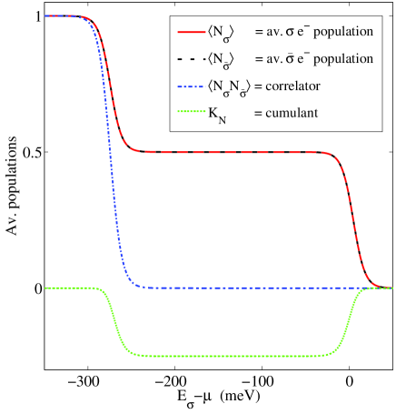
Figure 2: (Color online) Electron populations (for spin up, $\sigma=1$, in red, for spin down, $\sigma=2$, in dashed black), populations correlator (dotted-dashed intermediate purple curve), and cumulant (green dotted curve at the bottom) as functions of the energy of the nano-oscillator electron state.

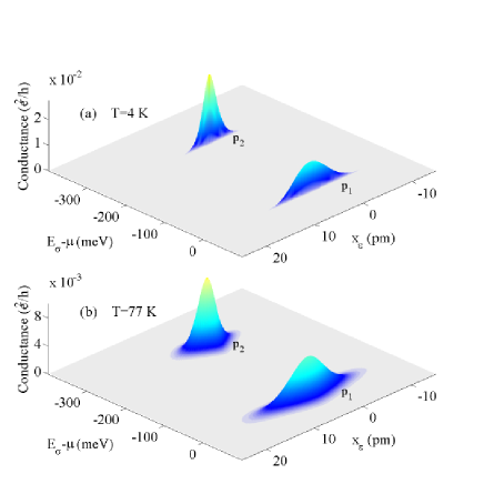
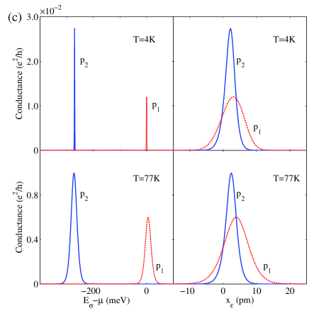
Figure 3: (Color online) Conductance of the nano-oscillator as a function of the state energy $(E_{\sigma}-\mu)$ and the oscillator shift $x_{\cal E}$ in an external electric field ${\cal E}$, with a tunneling length $\lambda=4$ pm, $h\Gamma_{L}$ = 0.1 meV and $h\Gamma_{R}$ = 0.002 meV for (a) $T=4$ K and (b) $T=77$ K. (c) Left: projections to the “$G$ versus $(E_{\sigma}-\mu)$” plane. Right: projections to the “$G$ versus $x_{\cal E}$” plane. The dashed red (continuous blue) peak p₁ (p₂) denotes the conductance peak at $E_{\sigma}=\mu$ ($E_{\sigma}=\mu-U_{0}$). When $x_{\cal E}=0$, p₁ and p₂ have an equal conductance, corresponding to the usual Coulumb blockade results.

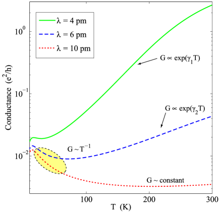
Figure 4: (Color online) Temperature dependence of the conductance $G(T)$ for various tunneling lengths $\lambda$ and for an oscillator shift $x_{\cal E}=0$. The yellow (shadowed) ellipse is the low-temperature regime where $G\sim T^{-1}$.

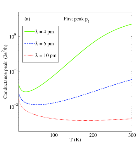
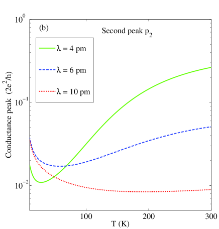
Figure 5: (Color online) Temperature dependence of the conductance $G(T)$ (for various tunneling lengths $\lambda$ and for an oscillator shift $x_{\cal E}=5$ pm) for (a) p₁ at $E_{\sigma}=\mu$ and (b) p₂ at $E_{\sigma}=\mu-U_{0}$. The conductance can vary orders of magnitude for small changes in $\lambda$.

References

• (1) For recent reviews on nano-oscillators and molecular junctions, see, e.g., R. I. Shekhter, Yu. Galperin, L. Y. Gorelik, A. Isacsson, and M. Jonson, J. Phys.: Condens. Matter 15, R441 (2003); M. Blencowe, Phys. Rep. 395, 159, 2004; M. Galperin, M. A. Ratner, and A. Nitzan, cond-mat/0612085.
• (2) L. Y. Gorelik, A. Isacsson, M. V. Voinova, B. Kasemo, R. I. Shekhter, and M. Jonson, Phys. Rev. Lett. 80, 4526 (1998); C. Weiss and W. Zwerger, Europhys. Lett. 47, 97 (1999); D. Mozyrsky and I. Martin, Phys. Rev. Lett. 89, 018301 (2002); A. D. Armour and A. MacKinnon, Phys. Rev. B 66, 035333 (2002); T. Novotny, A. Donarini, and A.-P. Jauho, Phys. Rev. Lett. 90, 256801 (2003); D. Fedorets, Phys. Rev. B 68, 033106 (2003); D. Fedorets, L. Y. Gorelik, R. I. Shekhter, and M. Jonson, Phys. Rev. Lett. 92, 166801 (2004); Y. Xue and M. A. Ratner, Phys. Rev B. 70, 155408 (2004).
• (3) K. D. McCarthy, N. Prokof’ev, and M. T. Tuominen, Phys. Rev. B 67, 245415 (2003).
• (4) L.F. Wei, Y.X. Liu, C.P. Sun, F. Nori, Phys. Rev. Lett. 97, 237201 (2006); S. Savel’ev, A.L. Rakhmanov, X. Hu, A. Kasumov, F. Nori, Phys. Rev. B 75, 165417 (2007).
• (5) H. Park, J. Park, A. K. L. Lim, A. H. Anderson, A. P. Alivisatos, and P. L. McEuen, Nature 407, 58 (2000).
• (6) A. Erbe, C. Weiss, W. Zwerger, and R. H. Blick, Phys. Rev. Lett. 87, 096106 (2001); D. V. Scheible and R. H. Blick, Appl. Phys. Lett. 84, 4632 (2004); Y. Majima, Y. Azuma, and K. Nagano, Appl. Phys. Lett. 87, 163110 (2005).
• (7) A. Yu. Smirnov, L. G. Mourokh, and N. J. M. Horing, Phys. Rev. B 67, 115312 (2003).
• (8) A. Yu. Smirnov, L. G. Mourokh, and N. J. M. Horing, Phys. Rev. B 69, 155310 (2004).
• (9) S. Braig and K. Flensberg, Phys. Rev. B 68, 205324 (2003).
• (10) F. Pistolesi and R. Fazio, Phys. Rev. Lett. 94, 036806 (2005).
• (11) J. Twamley, D. W. Utami, H.-S. Goan, and G. Milburn, New J. Phys. 8, 63 (2006).
• (12) S. Satpathy, Solid St. Comm. 112, 195 (1999).
• (13) T. Hotta, Phys. Rev. Lett. 96, 197201 (2006).
• (14) A. Mitra, I. Aleiner, and A. J. Millis, Phys. Rev. B 69, 245302 (2004); J. Koch and F. von Oppen, Phys. Rev. Lett. 94, 206804 (2005); H. Hübner and T. Brandes, arXiv: 0705.2728.
• (15) W. B. Davis, M. A. Ratner, and M. R. Wasiliewsky, J. A. Chem. Soc. 123, 7877 (2001).
• (16) N. Noginova, G. B. Loutts, E. S. Gillman, V. A. Atsarkin, and A. A. Verevkin, Phys. Rev. B 63 174414 (2001); N. Noginova, private communications.
• (17) U. Lundin and R. H. McKenzie, Phys. Rev. B 66, 075303 (2002).
Refer to caption