Two-dimensional spin-filtered chiral network model for the $\mathbb{Z}^{\ }_{2}$ quantum spin-Hall effect

Abstract

The effects of static disorder on the $\mathbb{Z}^{\ }_{2}$ quantum spin-Hall effect for non-interacting electrons propagating in two-dimensional space are studied numerically. A two-dimensional time-reversal symmetric network model is constructed to account for the effects of static disorder on the propagation of non-interacting electrons subjected to spin-orbit couplings. This network model is different from past network models belonging to the symplectic symmetry class in that the propagating modes along the links of the network can be arranged into an odd number of Kramers doublet. It is found that (1) a two-dimensional metallic phase of finite extent is embedded in a $\mathbb{Z}^{\ }_{2}$ insulating phase in parameter space and (2) the quantum phase transitions between the metallic and $\mathbb{Z}^{\ }_{2}$ insulating phases belong to the conventional symplectic universality class in two space dimensions.

I Introduction

An early triumph of quantum mechanics applied to the theory of solids was the understanding that, in the thermodynamic limit, the metallic state can be distinguished from the insulating state based on the energy spectrum of non-interacting electrons subject to the (static) periodic crystalline potential. The Bloch insulating state occurs when the chemical potential falls within the energy gap between the electronic Bloch bands while the metallic state follows otherwise.

It took another 50 years with the experimental discovery of the integer quantum Hall effectReviewIQHE to realize that a more refined classification of the Bloch insulating state follows from the sensitivity of occupied Bloch states to changes in the boundary conditions. A two-dimensional electron gas subjected to a strong magnetic field turns into a quantum Hall insulating state characterized by a quantized Hall conductance in units of $e^{2}/h$.Laughlin81 ; Halperin82 ; Thouless82 ; Avron83 ; Kohmoto85 ; Niu85 ; Arovas88 ; Hatsugai93 The topological texture of the quantum Hall insulating state manifests itself through the existence of chiral edge states:Halperin82 energy eigenstates that propagate in one direction along the boundary of a sample with strip geometry. On the other hand, the topologically trivial Bloch insulating state is insensitive to modification of boundary conditions and, therefore, it does not support gapless edge states in a strip geometry. The breaking of time-reversal symmetry by the magnetic field in the integer quantum Hall effect implies the chirality of edge states: all edge states propagate in the same direction. Chiral edge states thus cannot be back-scattered into counter propagating edge states by impurities. For this reason the quantization of the Hall conductance is insensitive to the presence of (weak) disorder.Halperin82 (Strong disorder destroys the very existence of edge states.)

The (global) breaking of time-reversal symmetry is not, strictly speaking, necessary for integer quantum Hall-like physics. As a thought experiment, one can consider, for example, a noninteracting two-component electronic gas with each component subjected to a magnetic-like field of equal magnitude but opposite direction.Freedman04 Each (independent) component is then characterized by its quantized Hall conductance. The arithmetic average of the two quantized Hall conductances vanishes while their difference is quantized in units of $2e^{*2}/h$ with $e^{*}$ the effective conserved charge. Bernevig and Zhang in Ref. Bernevig05, suggested along these lines that, for some semiconductors with time-reversal symmetric noninteracting Hamiltonians, the role of the magnetic field is played by the intrinsic spin-orbit coupling while the quantum number that distinguishes the two components of the two-dimensional noninteracting electronic gas is the electronic spin.Bernevig05 If so, the quantized Hall conductance for the electric charge (arithmetic average) vanishes while the quantized Hall conductance for the spin (difference) is nonvanishing (see Fig. 1).

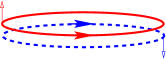
Figure 1: (Color online:) In the proposal of Ref. Bernevig05, , a spin-up edge state (full line) and a spin-down edge state (dashed line) at the boundary of a two-dimensional electronic droplet propagate with opposite velocities. The quantized Hall conductance for the charge vanishes while that for the spin is nonvanishing.

In the proposal of Bernevig and Zhang, independent quantization of the Hall conductance for each spin requires two independent $U(1)$ conserved currents. The first one follows from charge conservation. The second one follows from conservation of the spin quantum number perpendicular to the interface in which the electrons are confined. However, while the intrinsic spin-orbit coupling breaks the $SU(2)$ spin symmetry down to its $U(1)$ subgroup, the underlying symmetry responsible for the quantization of the spin-Hall conductance in Ref. Bernevig05, , other spin-orbit couplings such as the Rashba spin-orbit coupling break this leftover $U(1)$ spin symmetry. This is not to say that an unquantized quantum spin Hall effect cannot be present if the counterpropagating edge states survive the breaking of the residual $U(1)$ spin symmetry. However, a physical mechanism different from the one protecting the integer quantum Hall effect must then be invoked for these edge states to be robust against (weak) disorder.Zirnbauer92 ; Brouwer96 ; Suzuura02a ; Suzuura02b ; Takane04 ; Kane05a ; Kane05b ; Sheng05 ; Cenke06 ; CongjunWu06 ; Sheng06

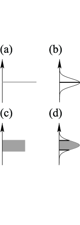
Figure 2: Qualitative plot of the bulk single-particle density of state (DOS) as a function of the chemical potential for (a) the integer quantum Hall effect without disorder, (b) the integer quantum Hall effect with weak disorder, (c) the $\mathbb{Z}^{\ }_{2}$ quantum spin-Hall state without disorder, and (d) the $\mathbb{Z}^{\ }_{2}$ quantum spin-Hall state with weak disorder. The chemical potential runs along the vertical axis while the DOS runs along the horizontal axis. The gray and white in these figures denote extended and localized states, respectively. The black straight lines in (b) and (d) denote the critical energies at which a quantum phase transition takes place between two Hall insulating states for (b) and between a metallic and an insulating state for (d).

Kane and Mele showed in Refs. Kane05a, and Kane05b, that a noninteracting tight-binding Hamiltonian inspired from graphene, with a staggered chemical potential and with translation invariant intrinsic and extrinsic (Rashba) spin-orbit couplings, realizes a time-reversal symmetric insulating state that they dubbed the $\mathbb{Z}^{\ }_{2}$ quantum spin-Hall state, provided the chemical potential lies within the bulk spectral gap (see Fig. 2). Although the $SU(2)$ spin symmetry is completely broken in most of coupling space, parameter space can nevertheless be divided into two regions depending on whether the number of Kramers doublet localized at the edges in a strip geometry is even or odd. The dispersion of one Kramers doublet edge state must necessarily cross the gap in the bulk of the sample when the number of Kramers doublet edge state is odd, in which case it supports an intrinsic quantum spin-Hall effect: an electric field induces a spin accumulation on the edges transverse to the direction of the electric field. This insulating state with an odd number of Kramers edge state defines the $\mathbb{Z}^{\ }_{2}$ quantum spin-Hall state. It displays a topological texture different from that of the integer quantum Hall state.Kane05b ; Sheng06 ; Roy06 ; Moore06 The insulating state with an even number of Kramers edge state is a conventional Bloch insulator.

The effect of disorder is to fill the gap in the bulk spectrum of the (clean) $\mathbb{Z}^{\ }_{2}$ quantum spin-Hall state. Sufficiently strong disorder is expected to wash out the $\mathbb{Z}^{\ }_{2}$ quantum spin-Hall state by removing the edge states very much in the same way as strong disorder does in the integer quantum Hall effect. On the other hand, Kane and Mele have argued that the $\mathbb{Z}^{\ }_{2}$ quantum spin-Hall state is robust to a weak time-reversal symmetric disorder, as a single Kramers doublet cannot undergo back-scattering by a time-reversal symmetric impurity. Both expectations were confirmed by a numerical study of (i) the four-probe Landauer-Büttiker and Kubo formulaSheng05 and of (ii) the spectral flow induced by changes in the twisted boundary conditions.Sheng06 By appealing to the symplectic symmetry of the Kane-Mele Hamiltonian, tuning the value of the chemical potential away from the tails of the disorder-broaden bands towards their center should trigger a disorder-induced transition to a metallic state (see the two mobility edges below and above the metallic state in Fig. 2).Hikami80 Onoda, Avishai, and Nagaosa have raised the possibility that the topological nature of the insulating phase might affect critical properties at this transition.Onoda06 Using standard techniquesMacKinnon83 to investigate the existence of mobility edges in tight-binding Hamiltonian perturbed by on-site disorder (here the Kane-Mele Hamiltonian with random on-site energies distributed with a box distribution), Onoda et al. deduced the existence of a mobility edge separating the $\mathbb{Z}^{\ }_{2}$ quantum spin-Hall state from a metallic state characterized by the exponent $\nu\approx 1.6$ for the diverging localization length. This exponent is different from the value $2.5\lesssim\nu\lesssim 2.8$ Merkt98 ; Asada02 that characterizes the conventional mobility edge in the two-dimensional symplectic universality class.

Figure 3: A network model is a collection of equipotential lines (of the disorder potential) and nodes. Equipotential lines are closed in the bulk and possibly open at the boundaries. In this paper, equipotential lines are the boundaries of identical squares with rounded corners while nodes are the midpoints between adjacent rounded corners. Edge states propagate anticlockwise (full lines) or clockwise (dashed lines) along equipotential lines if their spin is up or down, respectively. Each pair of edge state along an equipotential line can be arranged into a single Kramers doublet. Edge states belonging two two different equipotential line can exchange their momenta or spin at the nodes of the network such as S or $\textsf{S}^{\prime}$. Each node is thus assigned a $4\times 4$ unitary scattering matrix. Two independent copies of the Chalker-Coddington network model are obtained in the limit in which all the $4\times 4$ scattering matrices are diagonal with respect to the spin degrees of freedom.

Critical properties at the plateau transition in the integer quantum Hall effect are the same for two very different microscopic models. There is the effective tight-binding model with random off-diagonal matrix elements in the basis of Landau wave functions describing the lowest Landau level.Huckestein90 ; Huckestein95 There is the Chalker-Coddington network model valid for disorder potentials that vary smoothly on the scale of the cyclotron length.Chalker88 This agreement supports the notion that, for the problem of Anderson localization, disorder-induced continuous quantum phase transitions fall into universality classes determined by dimensionality, intrinsic symmetry, and topology. Furthermore, some network models have provided useful theoretical insights into the problem of Anderson localization and some have even been tractable analytically.Kramer05 The purpose of this paper is to construct a network model that realizes a quantum critical point separating the $\mathbb{Z}^{\ }_{2}$ quantum spin-Hall state from a metallic state. From this point of view, the network model for the two-dimensional symplectic universality class introduced in Ref. Merkt98, is unsatisfactory as it is built from an even number (two) of Kramers doublets propagating along the links of the network. Instead, the network model that we define in Sec. II has a single Kramers doublet propagating along the links of the network. Spin is a good quantum number along the links of the network so that the spin-up and spin-down components of the Kramers doublet can be assigned opposite velocities (chiralities). Scattering takes place at the nodes of the network. If the scattering matrix is diagonal in spin space, the network model realizes the proposal of Bernevig and Zhang: two copies of the Chalker-Coddington network model for the integer quantum Hall effect arranged so as not to break (global) time-reversal symmetry (see Fig. 1). However, we will only demand that the scattering matrix at a node respects time-reversal symmetry, i.e., it can completely break spin-rotation symmetry. Randomness is introduced through a spin-independent $U(1)$ random phase along the links. We also treat the cases of random and non-random scattering matrices at the nodes. In either cases, our spin-filtered chiral network model captures a continuous quantum phase transition between the $\mathbb{Z}^{\ }_{2}$ quantum spin-Hall state and the metallic state. We find in Sec. III the scaling exponent $\nu\approx 2.7$ for the localization length that is different from the exponent $\nu\approx 1.6$ seen by Onoda et al. but agrees with the conventional scaling exponent in the two-dimensional symplectic universality class.

II Definition

To represent the effect of static disorder on the coherent propagation of electronic waves constrained to a two-dimensional plane and subject to a strong magnetic field perpendicular to it, Chalker and Coddington introduced a chiral network model in Ref. Chalker88, . The Chalker-Coddington network model makes three assumptions. The disorder is smooth relative to the characteristic microscopic scale: the cyclotron length. Equipotential lines of the disorder potential define the boundaries of mesoscopic quantum Hall droplets along which chiral edge states propagate coherently. Edge states belonging to distinct equipotential lines can only undergo a unitary scattering process by which momenta is exchanged provided the distance between the two equipotential lines is of order of the cyclotron length. Such instances are called nodes of the network model.

We are seeking a network model that describes coherent propagation of electronic waves in a random medium that preserves time-reversal symmetry but breaks spin-rotation symmetry, in short a symplectic network model. A second condition is that the number of edge states that propagate along equipotential lines can be arranged into an odd number of Kramers doublet. We choose the number of Kramers doublet to be one for simplicity. A third condition is that the symplectic network model reduces to two independent Chalker-Coddington models in some region of parameter space. The symplectic network model from Ref. Merkt98, does not fulfill the last two conditions.

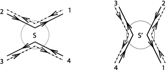
Figure 4: There are two nonequivalent nodes $\mathsf{S}$ and $\mathsf{S}^{\prime}$ from the point of view of the transfer matrix. Spin-up (full line) and spin down (dashed line) are good quantum numbers on the links but need not be conserved by the scattering at the nodes.

Given the last condition, it is natural to start with spin-filtered edge states moving along equipotential lines of the disorder potential depicted as squares with rounded corners as is done in Fig. 3. The third condition on the symplectic network model is then satisfied when all the $4\times 4$ unitary scattering matrices at nodes of the network do not couple edge states represented by the arrows along the full lines with edge states represented by the arrows along the dashed lines in Fig. 3. The first two conditions are otherwise satisfied when all the scattering matrices at the nodes of the network model from Fig. 3 are the most general $4\times 4$ unitary matrices that respect time-reversal symmetry. Without loss of generality we choose a node of type $\mathsf{S}$ from Fig. 3. The most general $4\times 4$ unitary scattering matrix that respects time-reversal symmetry is given by

$$\begin{split}&\begin{pmatrix}\psi^{(\mathrm{o})}_{1\uparrow}\\ \psi^{(\mathrm{o})}_{2\downarrow}\\ \psi^{(\mathrm{o})}_{3\uparrow}\\ \psi^{(\mathrm{o})}_{4\downarrow}\end{pmatrix}=S\begin{pmatrix}\psi^{(\mathrm{i})}_{2\uparrow}\\ \psi^{(\mathrm{i})}_{1\downarrow}\\ \psi^{(\mathrm{i})}_{4\uparrow}\\ \psi^{(\mathrm{i})}_{3\downarrow}\end{pmatrix},\\ &S=\left(\begin{array}[]{cc}r\sigma^{\ }_{0}&tQ\\ -tQ^{{\dagger}}&r\sigma^{\ }_{0}\end{array}\right),\ \left(\begin{array}[]{cc}\sigma^{\ }_{2}&0\\ 0&\sigma^{\ }_{2}\end{array}\right)S^{*}\left(\begin{array}[]{cc}\sigma^{\ }_{2}&0\\ 0&\sigma^{\ }_{2}\end{array}\right)=S^{\dagger},\\ &r=\tanh x,\qquad t=\frac{1}{\cosh x},\\ &Q={i}\sigma^{\ }_{0}\cos\theta\sin\varphi^{\ }_{1}+\sigma^{\ }_{1}\sin\theta\cos\varphi^{\ }_{2}\\ &\hphantom{Q=}-\sigma^{\ }_{2}\sin\theta\sin\varphi^{\ }_{2}+\sigma^{\ }_{3}\cos\theta\cos\varphi^{\ }_{1},\end{split}$$ (1)

with the labeling of incoming and outgoing scattering states given in Fig. 4. The structure displayed by Eq. (1) can be understood as follows. First, the amplitude for an incoming spin-filtered edge state not to tunnel must be spin-independent and thus parametrized by the single real number $r$. Second, the strength of quantum tunneling at a node can be parametrized by the positive-valued transmission amplitude $t$ that multiplies the purely imaginary quaternion $Q$. The purely imaginary quaternion acts on the spin-1/2 degrees of freedom through the unit $2\times 2$ matrix $\sigma^{\ }_{0}$ and the Pauli matrices $\sigma^{\ }_{1,2,3}$ and must therefore depend on four real parameters. Third, the local gauge transformation $S\to U^{{\dagger}}\,S\,U$ with $U=\mathrm{diag}\left(\begin{array}[]{cccc}e^{+{i}\phi^{\ }_{1}}&e^{-{i}\phi^{\ }_{1}}&e^{+{i}\phi^{\ }_{2}}&e^{-{i}\phi^{\ }_{2}}\end{array}\right)$ can absorb the dependence of $Q$ on the two independent phase shifts $0\leq\varphi^{\ }_{1,2}<2\pi$ compatible with time-reversal symmetry. At last unitarity delivers the constraints $r^{2}+t^{2}=1$ and $QQ^{{\dagger}}=\sigma^{\ }_{0}$. Up to an overall sign of $S$ and a local gauge transformation, $S$ can thus be parametrized by

$$\big{\{}(x,\theta)\,\big{|}\,0\leq x\leq\infty,\qquad 0\leq\theta\leq\pi/2\big{\}}.$$ (2)

The boundary $x=\infty$ for which the transmission amplitude vanishes and the scattering matrix is diagonal defines the classical limit of the network model. Quantum tunneling between neighboring plaquettes in Fig. 3 is very weak when $x\gg 1$. In this limit, the network model can be interpreted as follows. The host $\mathbb{Z}^{\ }_{2}$ quantum spin-Hall state, i.e., the translation invariant bulk state that supports an odd number of Kramers doublet edge states in a confined geometry free of disorder, breaks down into droplets of $\mathbb{Z}^{\ }_{2}$ quantum spin-Hall states separated by smooth random potential barriers. To appreciate the role played by the parameter $0\leq\theta\leq\pi/2$, we now consider different values of $x$ and $\theta$ on the boundary of parameter space. To this end, it is more convenient to replace the scattering matrix by two transfer matrices.

Nodes of type S in Figs. 3 and 4 are assigned the transfer matrix $\widetilde{\mathcal{M}}$,

$$\begin{split}&\left(\begin{array}[]{c}\psi^{\ }_{1\uparrow}\\ \psi^{\ }_{1\downarrow}\\ \psi^{\ }_{4\uparrow}\\ \psi^{\ }_{4\downarrow}\end{array}\right)=\widetilde{\mathcal{M}}\left(\begin{array}[]{c}\psi^{\ }_{2\uparrow}\\ \psi^{\ }_{2\downarrow}\\ \psi^{\ }_{3\uparrow}\\ \psi^{\ }_{3\downarrow}\end{array}\right),\qquad\widetilde{\mathcal{M}}=U\,\mathcal{M}\,U^{{\dagger}},\\ &U=\mathrm{diag}\left(\begin{array}[]{cccc}e^{+\frac{i}{2}(\varphi^{\ }_{1}+\varphi^{\ }_{2})}&e^{-\frac{i}{2}(\varphi^{\ }_{1}+\varphi^{\ }_{2})}&e^{-\frac{i}{2}(\varphi^{\ }_{1}-\varphi^{\ }_{2})}&e^{+\frac{i}{2}(\varphi^{\ }_{1}-\varphi^{\ }_{2})}\end{array}\right),\\ &\mathcal{M}=\frac{2}{\cosh 2x-\cos 2\theta}\begin{pmatrix}\sinh x\ \cosh x&\sin\theta\ \cos\theta&\sinh x\ \cos\theta&\cosh x\ \sin\theta\\ -\sin\theta\ \cos\theta&\sinh x\ \cosh x&-\cosh x\ \sin\theta&\sinh x\ \cos\theta\\ \sinh x\ \cos\theta&\cosh x\ \sin\theta&\sinh x\ \cosh x&\sin\theta\ \cos\theta\\ -\cosh x\ \sin\theta&\sinh x\ \cos\theta&-\sin\theta\ \cos\theta&\sinh x\ \cosh x\end{pmatrix}.\end{split}$$ (3a)

Nodes of type $$\textsf{S}^{\prime} \widetilde{\mathcal{M}}^{\prime}$$ in Fig. 3 are assigned the transfer matrix ,

$$\begin{split}&\left(\begin{array}[]{c}\psi^{\ }_{2\uparrow}\\ \psi^{\ }_{2\downarrow}\\ \psi^{\ }_{1\uparrow}\\ \psi^{\ }_{1\downarrow}\end{array}\right)=\widetilde{\mathcal{M}}^{\prime}\left(\begin{array}[]{c}\psi^{\ }_{3\uparrow}\\ \psi^{\ }_{3\downarrow}\\ \psi^{\ }_{4\uparrow}\\ \psi^{\ }_{4\downarrow}\end{array}\right),\qquad\widetilde{\mathcal{M}}^{\prime}=U^{\ }_{1}\,\mathcal{M}^{\prime}\,U^{\ }_{2},\\ &U^{\ }_{1}=\mathrm{diag}\left(\begin{array}[]{cccc}e^{+\frac{i}{2}(\varphi^{\ }_{1}+\varphi^{\ }_{2})}&e^{-\frac{i}{2}(\varphi^{\ }_{1}+\varphi^{\ }_{2})}&e^{+\frac{i}{2}(\varphi^{\ }_{1}+\varphi^{\ }_{2})}&e^{-\frac{i}{2}(\varphi^{\ }_{1}+\varphi^{\ }_{2})}\end{array}\right),\\ &U^{\ }_{2}=\mathrm{diag}\,\left(\begin{array}[]{cccc}e^{+\frac{i}{2}(\varphi^{\ }_{1}-\varphi^{\ }_{2})}&e^{-\frac{i}{2}(\varphi^{\ }_{1}-\varphi^{\ }_{2})}&e^{+\frac{i}{2}(\varphi^{\ }_{1}-\varphi^{\ }_{2})}&e^{-\frac{i}{2}(\varphi^{\ }_{1}-\varphi^{\ }_{2})}\end{array}\right),\\ &\mathcal{M}^{\prime}=\begin{pmatrix}-\cosh x\ \cos\theta&\sinh x\ \sin\theta&\sinh x\ \cos\theta&-\cosh x\ \sin\theta\\ -\sinh x\ \sin\theta&-\cosh x\ \cos\theta&\cosh x\ \sin\theta&\sinh x\ \cos\theta\\ -\sinh x\ \cos\theta&\cosh x\ \sin\theta&\cosh x\ \cos\theta&-\sinh x\ \sin\theta\\ -\cosh x\ \sin\theta&-\sinh x\ \cos\theta&\sinh x\ \sin\theta&\cosh x\ \cos\theta\end{pmatrix}.\end{split}$$ (3b)

Here, the convention for initial and final scattering states is given in Fig. 4. One verifies that, for all values of $0\leq\varphi^{\ }_{1,2}<2\pi$, $0\leq x\leq\infty$, and $0\leq\theta\leq\pi/2$ that parametrize $\widetilde{\mathcal{M}}$ and $\widetilde{\mathcal{M}}^{\prime}$, the conditions for pseudo-unitary

$$\mathcal{A}\begin{pmatrix}+\sigma^{\ }_{3}&0\\ 0&-\sigma^{\ }_{3}\end{pmatrix}\mathcal{A}^{\dagger}=\begin{pmatrix}+\sigma^{\ }_{3}&0\\ 0&-\sigma^{\ }_{3}\end{pmatrix}$$ (4)

and time-reversal symmetry

$$\begin{pmatrix}i\sigma^{\ }_{2}&0\\ 0&i\sigma^{\ }_{2}\end{pmatrix}\mathcal{A}\begin{pmatrix}-i\sigma^{\ }_{2}&0\\ 0&-i\sigma^{\ }_{2}\end{pmatrix}=\mathcal{A}^{*}$$ (5)

hold ($\mathcal{A}=\mathcal{M}$ or $\mathcal{M}^{\prime}$).

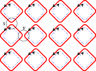
Figure 5: (Color online:) The network model at $\theta=0$ decouples into two networks depicted by the thick (red) and thin (blue) lines. Full and dashed lines distinguish propagation along the links of the networks of up and down spins, respectively.

Along the boundary $\theta=0$, the transfer matrices (3a) and (3b) reduce to

$$\mathcal{M}=\begin{pmatrix}\coth x&0&1/\sinh x&0\\ 0&\coth x&0&1/\sinh x\\ 1/\sinh x&0&\coth x&0\\ 0&1/\sinh x&0&\coth x\end{pmatrix}$$ (6a)

and

$$\mathcal{M}^{\prime}=\begin{pmatrix}-\cosh x\ &0&\sinh x&0\\ 0&-\cosh x&0&\sinh x\\ -\sinh x&0&\cosh x&0\\ 0&-\sinh x&0&\cosh x\end{pmatrix},$$ (6b)

respectively. As is depicted in Fig. 5, up and down spins have decoupled into two independent Chalker-Coddington models, each of which describes the integer quantum Hall plateau transition. Whenever $x=0$ or $x=\infty$ either $\mathcal{M}$ or $\mathcal{M}^{\prime}$ is diagonal so that edge states cannot escape the equipotential lines encircling the local extrema of the disorder potential. These are strongly insulating phases characterized by different integer topological (Chern) numbers; one for each spin direction. Across the plateau transition the number of edge states changes by one for each spin, and so does the number of Kramers doublet edge mode. This implies that the two insulating phases are distinct in the $\mathbb{Z}^{\ }_{2}$ classification. Quantum tunneling is strongest at the integer quantum Hall transition defined by the condition $\mathcal{M}\sim\mathcal{M}^{\prime}$ for which $x^{\ }_{\mathrm{cc}}=\ln(1+\sqrt{2})$. (By $\sim$ is meant equality in magnitude of all matrix elements.)

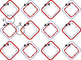
Figure 6: (Color online:) The network model at $\theta=\pi/2$ decouples into two networks depicted by the thick (red) and thin (blue) lines. Full and dashed lines distinguish propagation along the links of the networks of up and down spins, respectively.

Along the boundary $\theta=\pi/2$, the transfer matrices (3a) and (3b) reduce to

$$\mathcal{M}=\begin{pmatrix}\tanh x&0&0&1/\cosh x\\ 0&\tanh x&-1/\cosh x&0\\ 0&1/\cosh x&\tanh x&0\\ -1/\cosh x&0&0&\tanh x\end{pmatrix}$$ (7a)

and

$$\mathcal{M}^{\prime}=\begin{pmatrix}0&\sinh x&0&-\cosh x\\ -\sinh x&0&\cosh x&0\\ 0&\cosh x&0&-\sinh x\\ -\cosh x&0&\sinh x&0\end{pmatrix},$$ (7b)

respectively. The network model has decoupled into two independent network models as is depicted in Fig. 6. The $U(1)$ residual spin-rotation symmetry at $\theta=0$ is maximally broken by $\theta=\pi/2$. When $x=\infty$, $\mathcal{M}$ becomes diagonal while $\mathcal{M}^{\prime}$ is off-diagonal so that edge states cannot escape the equipotential lines encircling the local extrema of the disorder potential. The point $x=0$ is dominated by quantum tunneling since $\mathcal{M}\sim\mathcal{M}^{\prime}$ are then both anti-diagonal. (By $\sim$ is meant equality in magnitude of all matrix elements.) Furthermore, at $x=0$, propagation of Kramers doublets is ballistic along decoupled one-dimensional chiral channels. Each network model depicted in Fig. 6 belongs to the unitary universality class (without topological term) when $\theta=\pi/2$ and $0\leq x\leq\infty$. We thus anticipate an unstable fixed point at $x=0$ describing a metallic phase and an insulating phase for $x>0$.

Along the boundary $x=0$, the transfer matrices (3a) and (3b) reduce to

$$\mathcal{M}=\begin{pmatrix}0&\cot\theta&0&1/\sin\theta\\ -\cot\theta&0&-1/\sin\theta\ &0\\ 0&1/\sin\theta&0&\cot\theta\\ -1/\sin\theta&0&-\cot\theta&0\end{pmatrix}$$ (8a)

and

$$\mathcal{M}^{\prime}=\begin{pmatrix}-\cos\theta&0&0&-\sin\theta\\ 0&-\cos\theta&\sin\theta&0\\ 0&\sin\theta&\cos\theta&0\\ -\sin\theta&0&0&\cos\theta\end{pmatrix},$$ (8b)

respectively. The network model has decoupled into two independent network models as is depicted in Fig. 7. When $\theta=0$, $\mathcal{M}$ is off-diagonal while $\mathcal{M}^{\prime}$ is diagonal yielding a strongly insulating phase. The point $\theta=\pi/2$ is dominated by quantum tunneling since $\mathcal{M}\sim\mathcal{M}^{\prime}$ are then both anti-diagonal. (By $\sim$ is meant equality in magnitude of all matrix elements.) Furthermore, at $\theta=\pi/2$, propagation of Kramers doublets is ballistic along decoupled one-dimensional chiral channels. Each network model depicted in Fig. 7 belongs to the unitary universality class (without topological term) when $x=0$ and $0\leq\theta\leq\pi/2$. We thus anticipate an unstable fixed point at $\theta=\pi/2$ describing a metallic phase and an insulating phase for $0\leq\theta<\pi/2$.

Observe that the duality relation

$$\tanh x=\cos\theta$$ (9a)

implies that

$$\begin{split}&\mathcal{M}(x=0,\theta)\sim\mathcal{M}^{\prime}(x,\theta=\pi/2),\\ &\mathcal{M}^{\prime}(x=0,\theta)\sim\mathcal{M}(x,\theta=\pi/2).\end{split}$$ (9b)

(By $\sim$ is meant equality in magnitude of all matrix elements.)

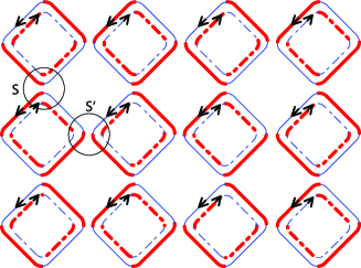
Figure 7: (Color online:) The network model at $x=0$ decouples into two networks depicted by the thick (red) and thin (blue) lines. Full and dashed lines distinguish propagation along the links of the networks of up and down spins, respectively.

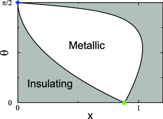
Figure 8: (Color online:) Expected phase diagram from the analysis of the network model along the boundaries of parameter space (2). The fixed point denoted by a filled (green) square along the boundary $\theta=0$ is the unstable quantum critical point located at $x^{\ }_{\mathrm{cc}}=\ln(1+\sqrt{2})$ separating two insulating phases in the Chalker-Coddington model. The fixed point denoted by the filled (blue) rhombus at the upper left corner is the unstable metallic phase. The shape of the metallic phase is controlled by the symmetry crossover between the unitary and symplectic symmetry classes.

From the analysis of the network model on the boundaries of parameter space, we deduce the qualitative phase diagram shown in Fig. 8. The numerics of Sec. III confirm the overall topology of this phase diagram.

The definition of the two-dimensional spin-filtered chiral network model for the $\mathbb{Z}^{\ }_{2}$ quantum spin-Hall effect is completed by specifying the boundary conditions. These are dictated by the numerical method that we shall use in Sec. III. Following MacKinnon and Kramer, we seek the transfer matrix of a long but narrow sample connected at both ends to semi-infinite ideal metallic leads. To minimize finite size effects, we impose periodic boundary conditions in the transverse direction. The transfer matrix is then a $4M\times 4M$ pseudo-unitary matrix that maps $4M$ plane waves from the left lead into $4M$ plane waves from the right lead that we define as follows. First, we consider a slice of the sample that we label by the integer $n=1,2,\ldots,N$ as is depicted in Fig. 9a ($N\gg 4M$). We assign to this slice the $4M\times 4M$ pseudo-unitary matrix $\mathcal{M}^{\ }_{\mathrm{sl}}(n)$,

$$\begin{split}&\mathcal{M}^{\ }_{\mathrm{sl}}(n):=\mathcal{M}^{\ }_{\mathsf{S}^{\prime}}(n)\ U^{(2)}_{\mathrm{sl}}(n)\ \mathcal{M}^{\ }_{\mathsf{S}}(n)\ U^{(1)}_{\mathrm{sl}}(n),\\ &U^{(1)}_{\mathrm{sl}}(n)=\mathrm{diag}\begin{pmatrix}e^{+i\phi^{(1)}_{1}(n)}&e^{-i\phi^{(1)}_{1}(n)}&\cdots&e^{+i\phi^{(1)}_{2M}(n)}&e^{-i\phi^{(1)}_{2M}(n)}\end{pmatrix},\\ &\mathcal{M}^{\ }_{\mathsf{S}}(n)=\begin{pmatrix}\mathcal{M}^{\ }_{00}(n)&0&\cdots&0&\mathcal{M}^{\ }_{0M}(n)\\ 0&\mathcal{M}^{\ }_{1}(n)&0&\cdots&0\\ \vdots&\ddots&\ddots&\ddots&\vdots\\ 0&\cdots&0&\mathcal{M}^{\ }_{M-1}(n)&0\\ \mathcal{M}^{\ }_{M0}(n)&0&\cdots&0&\mathcal{M}^{\ }_{MM}(n)\end{pmatrix},\\ &U^{(2)}_{\mathrm{sl}}(n)=\mathrm{diag}\begin{pmatrix}e^{+i\phi^{(2)}_{1}(n)}&e^{-i\phi^{(2)}_{1}(n)}&\cdots&e^{+i\phi^{(2)}_{2M}(n)}&e^{-i\phi^{(2)}_{2M}(n)}\end{pmatrix},\\ &\mathcal{M}^{\ }_{\mathsf{S}^{\prime}}(n)=\mathrm{diag}\begin{pmatrix}\mathcal{M}^{\prime}_{1}(n)&\cdots&\mathcal{M}^{\prime}_{M}(n)\end{pmatrix}.\end{split}$$ (10a)

Here, $$\mathcal{M}^{\ }_{m}(n) m=1,\ldots,M-1 \mathcal{M}^{\prime}_{m}(n) m=1,\ldots,M$$ with and with are given by Eqs. (3a) and (3b), respectively, while we have imposed periodic boundary conditions in the transverse direction with the choice

$$\mathcal{M}_{00}(n)=\mathcal{M}_{MM}(n)=\frac{2}{\cosh 2x-\cos 2\theta}\begin{pmatrix}\sinh x\cosh x&\sin\theta\cos\theta\\ -\sin\theta\cos\theta&\sinh x\cosh x\end{pmatrix},$$ (10b)

$$\mathcal{M}_{0M}(n)=\mathcal{M}_{M0}(n)=\frac{2}{\cosh 2x-\cos 2\theta}\begin{pmatrix}\sinh x\cos\theta&\sin\theta\cosh x\\ -\sin\theta\cosh x&\sinh x\cos\theta\end{pmatrix}.$$ (10c)

The phases $$\phi^{(l)}_{m}(n) l=1,2 m=1,\ldots,2M n=1,\ldots,N 0 2\pi$$ with , , and take values between and . Second, we assign to the quasi-one dimensional network model depicted in Fig. 9b the transfer matrix

$$\mathcal{M}^{\ }_{\mathrm{tot}}:=\prod_{n=1}^{N}\mathcal{M}^{\ }_{\mathrm{sl}}(n).$$ (10d)

This completes the definition of the two-dimensional spin-filtered chiral network model for the $\mathbb{Z}^{\ }_{2}$ quantum spin-Hall effect.

We close Sec. II by showing that $\mathcal{M}^{\ }_{\mathrm{tot}}$ belongs to the Lie group $SO^{*}(4M)$. By construction, flux conservation,

$$\mathcal{M}^{\ }_{\mathrm{tot}}\,\Sigma_{3}\,\mathcal{M}^{{\dagger}}_{\mathrm{tot}}=\Sigma^{\ }_{3},\qquad\Sigma^{\ }_{3}=\begin{pmatrix}\sigma^{\ }_{3}&0\\ 0&-\sigma^{\ }_{3}\end{pmatrix}\otimes I^{\ }_{M},$$ (11)

and time-reversal symmetry,

$$\Sigma^{\ }_{2}\,\mathcal{M}^{\ }_{\mathrm{tot}}\,\Sigma^{T}_{2}=\mathcal{M}^{*}_{\mathrm{tot}},\qquad\Sigma^{\ }_{2}=i\sigma^{\ }_{2}\otimes I^{\ }_{2M},$$ (12)

where $I^{\ }_{2M}$ is the $2M\times 2M$ unit matrix hold. It follows from Eq. (12) that

$$\mathcal{M}^{{\dagger}}_{\mathrm{tot}}=\Sigma^{\ }_{2}\,\mathcal{M}^{T}_{\mathrm{tot}}\,\Sigma^{T}_{2}.$$ (13)

Substituting Eq. (13) into Eq. (11) yields

$$\begin{split}&\mathcal{M}^{\ }_{\mathrm{tot}}\,\Sigma^{\ }_{1}\,\mathcal{M}^{T}_{\mathrm{tot}}=\Sigma^{\ }_{1},\\ &\Sigma^{\ }_{1}=\Sigma^{\ }_{3}\Sigma^{\ }_{2}=\begin{pmatrix}\sigma^{\ }_{1}&0\\ 0&-\sigma^{\ }_{1}\end{pmatrix}\otimes I^{\ }_{M}.\end{split}$$ (14)

We introduce the matrix

$$A=\frac{1}{\sqrt{2}}\begin{pmatrix}\sigma^{\ }_{2}+\sigma^{\ }_{3}&0\\ 0&\sigma^{\ }_{2}-\sigma^{\ }_{3}\end{pmatrix}\otimes I^{\ }_{M},$$ (15)

and write $\Sigma^{\ }_{1}=-iAA^{T}$. Equation (14) then reads

$$\widehat{\mathcal{M}}^{\ }_{\mathrm{tot}}\,\widehat{\mathcal{M}}^{T}_{\mathrm{tot}}=1,\qquad\widehat{\mathcal{M}}^{\ }_{\mathrm{tot}}=A\,\mathcal{M}^{\ }_{\mathrm{tot}}\,A,$$ (16)

where we have used the identity $A^{2}=1$. We can rewrite Eq. (11) in terms of $\widehat{\mathcal{M}}^{\ }_{\mathrm{tot}}$,

$$\begin{split}&\widehat{\mathcal{M}}^{\ }_{\mathrm{tot}}\,\Sigma^{\ }_{2}\,\widehat{\mathcal{M}}^{{\dagger}}_{\mathrm{tot}}=\Sigma^{\ }_{2},\\ &iA\,\Sigma^{\ }_{3}\,A=\begin{pmatrix}i\sigma^{\ }_{2}&0\\ 0&i\sigma^{\ }_{2}\end{pmatrix}\otimes I^{\ }_{M}=\Sigma^{\ }_{2}.\end{split}$$ (17)

With an orthogonal transformation that exchanges rows and columns, we can bring $\Sigma^{\ }_{2}$ into the form,

$$O\,\Sigma^{\ }_{2}\,O^{T}=\begin{pmatrix}0&I^{\ }_{2M}\\ -I^{\ }_{2M}&0\end{pmatrix}=J^{\ }_{2M}.$$ (18)

We thus conclude that $O\,\widehat{\mathcal{M}}^{\ }_{\mathrm{tot}}\,O^{T}$ is an element of the group $SO^{*}(4M)$ defined by the conditions,

$$g\,J^{\ }_{2M}\,g^{{\dagger}}=J^{\ }_{2M},\quad g\,g^{T}=I^{\ }_{4M},\quad g\in GL(4M,\mathbb{C}).$$ (19)

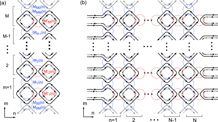
Figure 9: (Color online:) (a) A slice of the network model assuming periodic boundary conditions in the transverse direction, here represented by the gray links. (b) Wire geometry of the network model.

III Numerics

This section is devoted to a numerical study of the dependence of the smallest Lyapunov exponent of the transfer matrix $\mathcal{M}^{\ }_{\mathrm{tot}}$ defined in Eq. (10), as a function of the width $M$ of the quasi-one dimensional network model. Although $\mathcal{M}^{\ }_{\mathrm{tot}}$ is taken from a statistical ensemble that we will specify below, Lyapunov exponents are self-averaging random variables for an infinitely long quasi-one dimensional network model, $N\to\infty$.Johnston83 ; Brouwer96

The eigenvalues of the $4M\times 4M$ Hermitian matrix $\mathcal{M}^{{\dagger}}_{\mathrm{tot}}\,\mathcal{M}^{\ }_{\mathrm{tot}}$ are doubly degenerate and written as $\exp(\pm 2X_{j})$ with $0<X_{1}<X_{2}<\ldots<X_{M}$. The localization length $\xi^{\ }_{M}$ is then given by

$$\xi^{\ }_{M}=\lim_{N\to\infty}\frac{N}{X_{1}}.$$ (20)

The localization length $\xi^{\ }_{M}$ is a finite and self-averaging length scale that controls the exponential decay of the Landauer conductance for any fixed width $M$ of the infinitely long quasi-one dimensional network model, as the transfer matrix (10) belongs to the group $SO^{*}(4M)$.Brouwer96 It is of course impossible to study infinitely long quasi-one dimensional network models numerically and we shall approximate $\xi^{\ }_{M}$ with $\xi^{\ }_{M,N}$ obtained from the Lyapunov exponents of a finite but long quasi-one dimensional network model made of $N$ slices. In our numerics we have set $N=5\times 10^{5}\sim 8\times 10^{6}$.

As shown by MacKinnon and Kramer,MacKinnon83 criticality in two dimensions can be accessed from the dependence of the normalized localization length

$$\Lambda:=\xi^{\ }_{M}/M$$ (21)

on the width $M$ of the quasi-one dimensional network model. For example, if $\xi$ denotes the two-dimensional localization length and if $\xi$ diverges according to the power law

$$\xi\sim|z-z^{\ }_{c}|^{-\nu}$$ (22)

upon tuning of a single microscopic parameter $z$ close to its critical value $z^{\ }_{c}$, the singular part of $\Lambda$ as $M\to\infty$ should be given by a scaling functionSlevin99

$$\Lambda\sim F(\chi M^{1/\nu},\zeta M^{y},\ldots).$$ (23)

Here, $\chi$ and $\zeta$ are the single relevant and dominant irrelevant scaling variables, respectively.Cardy96 The largest irrelevant scaling exponent satisfies $y<0$. We assume that $F$ can be expanded in powers of $\zeta M^{y}$ and $\chi M^{1/\nu}$,

$$\begin{split}\Lambda\sim&\,\sum_{p=0}^{\infty}\sum_{q=0}^{\infty}F^{\ }_{p,q}\zeta^{p}\chi^{q}M^{py+q/\nu}\end{split}$$ (24)

where $F^{\ }_{p,q}\in\mathbb{R}$ are the expansion coefficients. We also assume that the relevant scaling variable $\chi$ is linearly related to $|z-z^{\ }_{c}|$ while the irrelevant scaling variable $\zeta$ is a constant in the vicinity of the critical point. Finally, for any given $0\leq\theta\leq\pi/2$ from the scattering matrix (1), we identify the microscopic parameter $z$ as the parameter $0\leq x\leq\infty$. This motivates the scaling ansatz

$$\begin{split}\Lambda=&\,\sum_{q=0}^{3}f^{(\theta)}_{0,q}\left(x-x^{(\theta)}_{c}\right)^{q}M^{q/\nu}\\ &\,+\sum_{q=0}^{2}f^{(\theta)}_{1,q}\left(x-x^{(\theta)}_{c}\right)^{q}M^{y+q/\nu}\end{split}$$ (25a)

with the 10 real-valued fitting parameters

$$\nu,\ y,\ x^{(\theta)}_{c},\ \Lambda^{(\theta)}_{c}:=f^{(\theta)}_{0,0},$$ (25b)

and

$$f^{(\theta)}_{0,1},\ f^{(\theta)}_{0,2},\ f^{(\theta)}_{0,3},\ f^{(\theta)}_{1,0},\ f^{(\theta)}_{1,1},\ f^{(\theta)}_{1,2}.$$ (25c)

Observe that single-parameter scaling is obeyed by

$$\Lambda^{\prime}:=\Lambda-\sum_{p=1}^{\infty}\sum_{q=0}^{\infty}F^{\ }_{p,q}\zeta^{p}\chi^{q}M^{py+q/\nu},$$ (26)

or, in practice,

$$\Lambda^{\prime}:= \,\Lambda-\sum_{q=0}^{2}f^{(\theta)}_{1,q}\left(x-x^{(\theta)}_{c}\right)^{q}M^{y+q/\nu}$$

$$= \,\sum^{3}_{q=0}f^{(\theta)}_{0,q}\left(x-x^{(\theta)}_{c}\right)^{q}M^{q/\nu}.$$ (27)

The values taken by the width $M$ of the quasi-one dimensional network model are $M=4,\,8,\,16,\,32,\,64$. To reduce the statistical error, average over $16$ different realizations of the disorder potential are calculated for any given ${M,x,\theta}$ when $\theta$ is not random and ${M,x}$ otherwise.

The disorder potential is modeled in two different ways, i.e., we introduce disorder in the transfer matrix (10) as follows. Case I: $0\leq\theta\leq\pi/2$ and $0\leq x\leq\infty$ are the same for all nodes and randomness is introduced by taking all the phases $\phi^{(l)}_{m}(n)$ with $l=1,2$, $m=1,\ldots,2M$, and $n=1,\ldots,N$ to be independently and uniformly distributed between $0$ and $2\pi$. Case II: in addition to the randomness in the phases $\phi^{(l)}_{m}(n)$ we allow $\theta$ to be independently distributed with the probability $\sin(2\theta)$ between $0$ and $\pi/2$ at each node of the network. As before, $0\leq x\leq\infty$ is the same for all nodes.

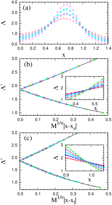
Figure 10: (Color online:) (a) Normalized localization length $\Lambda$ as a function of $x$ at fixed $\theta=3\pi/16$ for the widths $M=4$ (crosses), $M=8$ (open squares), $M=16$ (filled squares), $M=32$ (open circles), and $64$ (filled circles) of the quasi-one dimensional network. Error bars are much smaller than symbol sizes. There are two values of $x$ ($x^{\ }_{s}\approx 0.46$ and $x^{\ }_{l}\approx 0.97$) for which $\Lambda$ does not appear to depend on $M$. (b) A fit of the data shown in (a) with the help of the one-parameter scaling ansatz (27) when $x$ is close to $x^{\ }_{s}$. Inset: A blow up of (a) in the vicinity of $x^{\ }_{s}$. (c) A fit of the data shown in (a) with the help of the one-parameter scaling ansatz (27) when $x$ is close to $x^{\ }_{l}$. Inset: A blow up of (a) in the vicinity of $x^{\ }_{l}$.

Table 1: Critical exponent, normalized localization length, and (minimal) node parameter $x_{s}$ as a function of $\theta$. The poor agreement at $\theta=\pi/4$ is probably due to the presence of a large crossover length scale near the boundary $x=0$.

$\theta$	$\nu$	$\Lambda_{c}$	$x_{s}$
$\pi/8$	$2.85\pm 0.30$	$1.87\pm 0.09$	$0.667\pm 0.004$
$3\pi/16$	$2.77\pm 0.16$	$1.86\pm 0.02$	$0.465\pm 0.001$
$7\pi/32$	$2.73\pm 0.05$	$1.90\pm 0.01$	$0.244\pm 0.001$
$\pi/4$ *	$2.17\pm 0.21$	$1.82\pm 0.01$	$0.016\pm 0.001$

Table 2: Critical exponent, normalized localization length, and (maximal) node parameter $x_{l}$ as a function of $\theta$.

$\theta$	$\nu$	$\Lambda_{c}$	$x_{l}$
$\pi/8$	$2.78\pm 0.19$	$1.94\pm 0.10$	$0.972\pm 0.004$
$3\pi/16$	$2.73\pm 0.08$	$1.87\pm 0.03$	$0.970\pm 0.002$
$\pi/4$	$2.65\pm 0.06$	$1.84\pm 0.01$	$0.970\pm 0.002$
$3\pi/8$	$2.85\pm 0.10$	$1.78\pm 0.06$	$0.982\pm 0.002$

III.1 Case I: Randomness on the links only

We found two unstable fixed points on the boundaries of parameter space (2) and the expected phase diagram was shown in Fig. 8. Boundary $x=\infty$ realizes an insulating phase. Boundary $\theta=0$ realizes the plateau transition at $x^{\ }_{\mathrm{cc}}=\ln(1+\sqrt{2})$ between two Hall insulating phases in the integer quantum Hall effect. Boundaries $x=0$ and $\theta=\pi/2$ realize the unitary universality class with its insulating phase terminating at the unstable metallic point $(x,\theta)=(0,\pi/2)$. Any critical point close to the last three boundaries is difficult to identify numerically as characteristic crossover length scales between different universality classes become very large. A related difficulty comes about from the fact that the characteristic disorder strength can remain stronger than the characteristic strength of the spin-rotation symmetry breaking away from the boundary $\theta=0$ of parameter space.Ando89 For this reason, we use the scaling ansatz (27) to search for the phase boundaries in the interior of parameter space (2).

For illustration, we present in Fig. 10(a) the $x$ dependence of the normalized localization length $\Lambda$ for the fixed values of $\theta=3\pi/16$ and $M=4,8,16,32$. It is seen that $\Lambda$ increases with increasing $M$ for $x$ between $0.5$ and $0.9$. For fixed $0.5<x<0.9$, this is either the signature for an extended state or that for a localized state whose localization length is larger than the maximal width of the quasi-one dimensional network model. Conversely, for $x$ smaller than $0.5$ or larger than $0.9$, $\Lambda$ decreases with increasing $M$, i.e., this is the signature of a localized state. There appears to be two values of $x$, that we denote with $x^{\ }_{s}<x^{\ }_{l}$, for which $\Lambda$ does not depend on $M=4,8,16,32$, and hence are good candidates for a pair of critical points separating a metallic from an insulating phase. The inset of Fig. 10(b) [Fig. 10(c)] magnifies the dependence of $\Lambda$ on $M=4,8,16,32,64$ close to $x^{\ }_{s}$ ($x^{\ }_{l})$. On this scale $x^{\ }_{s}$ remains well-defined but not $x^{\ }_{l}$. We attribute the absence of a single crossing point $x^{\ }_{l}$ in the inset of Fig. 10(c) to a large contribution from an irrelevant scaling variable. This hypothesis is verified in Figs. 10(b) and 10(c) where the single-parameter dependence of $\Lambda^{\prime}$ on the scaling variable $M^{1/\nu}|x-x^{\ }_{s}|$ and $M^{1/\nu}|x-x^{\ }_{l}|$, respectively, is demonstrated (we found the value $y\approx-1$ for the largest irrelevant scaling exponent). The values of $\nu$, $\Lambda^{\ }_{c}$, $x^{\ }_{s}$, and $x^{\ }_{l}$ obtained from the scaling ansatz (27) for different values of $\theta$ can be found in Tables 1 and 2. The values that we obtain for $\nu$ and $\Lambda^{\ }_{c}$ are consistent with those for the standard two-dimensional symplectic universality class.Merkt98 ; Asada02 Our numerical map of the phase boundaries separating the metallic from the insulating phase in the parameter space (2) is shown in Fig. 11. The shape of the metallic region in Fig. 11 is controlled by the crossover from the unitary to the symplectic symmetry class.

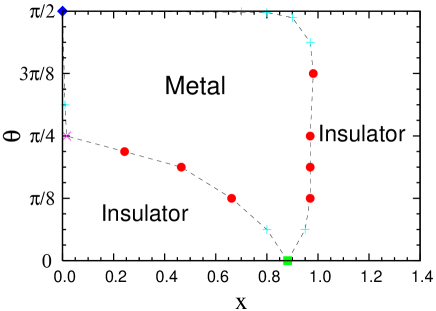
Figure 11: (Color online:) Phase diagram for the network model in the parameter space (2). The location of a critical point denoted by a filled (red) circle follows from the scaling ansatz (27). That denoted by a cross is a rougher estimate due to large symmetry crossover effects. The critical points denoted by a filled (green) square and a filled (blue) rhombus correspond to the critical points of the Chalker-Coddington network model and the unstable metallic fixed point from the unitary universality class, respectively. Dashed lines are guide to the eye.

The dependence of the normalized localization length $\Lambda$ on $\theta$ in the insulating regimes $x<\ln(1+\sqrt{2})$ and $x>\ln(1+\sqrt{2})$ are different as is shown in Fig. 12. In the small $\theta$ insulating regime $x<\ln(1+\sqrt{2})$ of Fig. 11, $\Lambda$ is an increasing function of $\theta$ for fixed $x$ and $M$, as is expected from the proximity of a phase boundary to a metallic phase. In the insulating regime $x>1>\ln(1+\sqrt{2})$ of Fig. 11, $\Lambda$ depends weakly on $\theta$ for fixed $x$ and $M$, as is expected from a strongly localized regime. When $x$ is held fixed at the Chalker-Coddington critical point $x^{\ }_{\mathrm{cc}}=\ln(1+\sqrt{2})$. $\Lambda$ is an increasing function of $\theta$ at fixed $M$ while $\Lambda$ is an increasing function of $M$ at fixed $\theta$. This is the expected behavior assuming that any finite $\theta$ drives the critical point $(x,\theta)=\big{(}\ln(1+\sqrt{2}),0\big{)}$ into a metallic phase. The duality relation (9) is also verified numerically in Fig. 12.

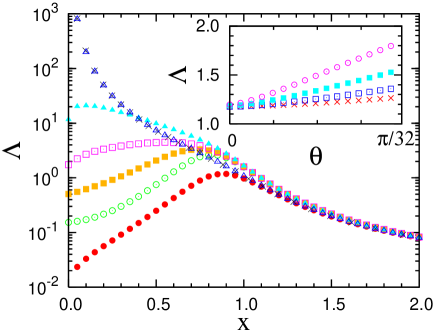
Figure 12: (Color online:) Logarithm of the normalized localization length $\Lambda$ as a function of $x$ at fixed $M=16$ for $\theta=0$ (filled circles), $\pi/8$ (open circles), $3\pi/16$ (filled squares), $\pi/4$ (open squares), $3\pi/8$ (filled triangles), and $\pi/2$ (open triangles). The duality relation (9) is verified by plotting the dependence of $\ln\Lambda$ on $\theta$ when $x=0$ and $M=16$ (crosses) as a function of $x=\mathrm{arctanh}(\cos\theta)$. Inset: Dependence of $\Lambda$ on $\theta$ for $x=\ln(1+\sqrt{2})$ and $M=4$ (crosses), $M=8$ (open squares), $M=16$ (filled squares), and $M=32$ (open circles).

III.2 Case II: Randomness on the links and nodes

Following Asada et al. in Ref. Asada02, , we expect that corrections due to irrelevant scaling variables should be reduced by choosing $\theta$ to be independently distributed between $0$ and $\pi/2$ with the probability $\sin(2\theta)$ for all nodes of the network. As is illustrated with Fig. 13, a metallic phase exists when $0.05<x<1.0$. There are two quantum critical points $x^{\ }_{s}<x^{\ }_{l}$ separating the metallic phase $x^{\ }_{s}<x<x^{\ }_{l}$ from the insulating phase. The scaling analysis must account for an irrelevant scaling variable with $y\approx-1$ in the vicinity of $x^{\ }_{s}$. In the vicinity of $x^{\ }_{l}$ a single-parameter scaling analysis suffices. Both scaling analysis, summarized in Table 3, imply that the critical points $x^{\ }_{s}\approx 0.05$ and $x^{\ }_{l}\approx 0.97$ belong to the standard symplectic universality class.

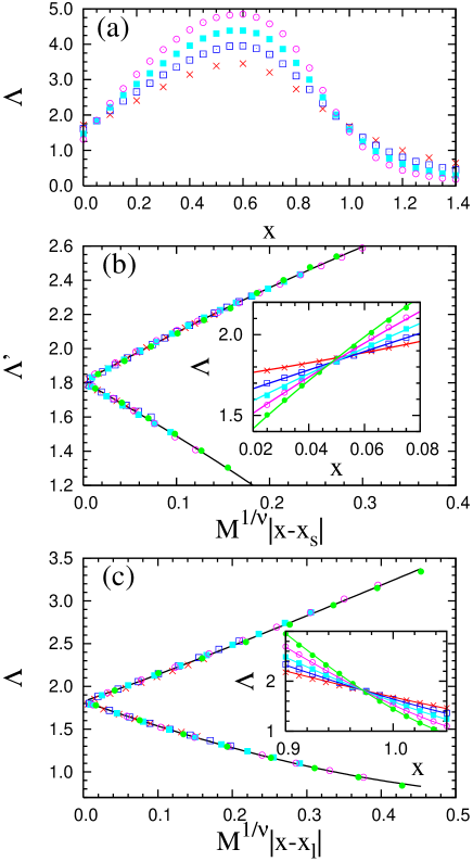
Figure 13: (Color online:) (a) Normalized localization length $\Lambda$ as a function of $x$ with a random $\theta$ for the widths $M=4$ (times), $M=8$ (open squares), $M=16$ (filled squares), $M=32$ (open circles), and $64$ (filled circles) of the quasi-one dimensional network. Error bars are much smaller than symbol sizes. There are two values of $x$ ($x^{\ }_{s}\approx 0.05$ and $x^{\ }_{l}\approx 0.97$) for which $\Lambda$ does not appear to depend on $M$. (b) A fit of the data shown in (a) with the help of the one-parameter scaling ansatz (27) (whereby $f^{(\theta)}_{q,q}\to f^{\ }_{q,q}$ for all $p,q\in\mathbb{N}$) when $x$ is close to $x^{\ }_{s}$. Inset: A blow up of (a) in the vicinity of $x^{\ }_{s}$. (c) A fit of the data shown in (a) with the help of the one-parameter scaling ansatz (25a) (whereby $f^{(\theta)}_{0,q}\to f^{\ }_{0,q}$ and $f^{(\theta)}_{1,q}=0$ for all $q\in\mathbb{N}$) when $x$ is close to $x^{\ }_{l}$. Inset: A blow up of (a) in the vicinity of $x^{\ }_{l}$.

Table 3: Critical exponent, normalized localization length, and node parameter when $\theta$ is distributed between $0$ and $\pi/2$.

	$\nu$	$\Lambda_{c}$	$x_{c}$
$x_{s}$	$2.74\pm 0.12$	$1.81\pm 0.01$	$0.047\pm 0.001$
$x_{l}$	$2.68\pm 0.06$	$1.82\pm 0.01$	$0.971\pm 0.001$

IV Summary

We have constructed and studied a two-dimensional spin-filtered chiral network model for the $\mathbb{Z}^{\ }_{2}$ quantum spin-Hall effect. Disorder has been implemented in two distinct ways. The quantum phase transitions between the insulating and metallic state are found to be characterized by the scaling exponent $\nu\approx 2.7$ for the diverging localization length. This value is consistent with that found in previous numerical studies of the two-dimensional metal to insulator transition in the symplectic universality class.Merkt98 ; Asada02 We did not find the value $\nu\approx 1.6$, recently observed by Onoda et al. in Ref. Onoda06, , that was interpreted as the signature of a new universality class at the transition between the $\mathbb{Z}^{\ }_{2}$ quantum spin-Hall insulating and the metallic state.

It is important to remember the similarities and differences between our network model and the lattice model studied in Ref. Onoda06, . Common to the two models is that, in the absence of disorder, they support a host $\mathbb{Z}^{\ }_{2}$ quantum spin-Hall state (a host $\mathbb{Z}^{\ }_{2}$ insulator for brevity) whereby an odd number of Kramers doublet edge states cause an accumulation of spin at the edges under an applied electric field. The crucial difference lies in the spatial correlation of the disorder potential added to the host $\mathbb{Z}^{\ }_{2}$ insulator. On the one hand, in Ref. Onoda06, disorder is introduced as a random on-site potential that has no spatial correlation. On the other hand, our network model is obtained by perturbing the host $\mathbb{Z}^{\ }_{2}$ insulator with a spatially smooth disorder potential that breaks the host $\mathbb{Z}^{\ }_{2}$ insulator into droplets of $\mathbb{Z}^{\ }_{2}$ insulators. The network model can thus be viewed as a coarse-grained effective model for $\mathbb{Z}^{\ }_{2}$ insulating droplets that are weakly coupled through quantum tunneling.

The intrinsic symmetry (time reversal) respected by the statistical ensemble of random Hamiltonians or scattering matrices is not changed by the range of the spatial correlation of the disorder. The hypothesis of universality would then suggest that the same critical scaling should be observed at the localization-delocalization transitions in the lattice model of Ref. Onoda06, and in our network model. The apparent violation of the universality by the two numerical results can be reconciled if one assumes that there is a long crossover length scale beyond which microscopic differences between the two models become irrelevant. Corrections from irrelevant scaling variables may strongly depend on the range of the disorder potential, as in the case of the plateau transition in the second Landau level,Huckestein94 and it could well be that the system sizes studied in Ref. Onoda06, were not large enough. Verification of this scenario is left for future work.

The fact that our network model is built out of two Chalker-Coddington network models coupled in a time-reversal invariant way has important consequences. Criticality in each Chalker-Coddington network model can be encoded by the field theory of a single (two-components) Dirac fermion coupled to a random vector potential, a random mass, and a random scalar potential.Ho96 It then follows by continuity (for small enough $\theta$) that the two lines of critical points emerging from the Chalker-Coddington critical point in Fig. 11 can be encoded by a field theory for two flavors of Dirac fermions. It is their coupling by disorder that prevents the emergence of a time-reversal symmetric and topologically driven quantum critical behavior.Ostrovsky07 ; Ryu07

References

- (1) For a review, see The Quantum Hall Effect, edited by R. E. Prange and S. M. Girvin (Springer-Verlag, Berlin, 1990).
- (2) R. B. Laughlin, Phys. Rev. B 23, 5632 (1981).
- (3) B. I. Halperin, Phys. Rev. B 25, 2185 (1982).
- (4) D. J. Thouless, M. Kohmoto, M. P. Nightingale, and M. den Nijs, Phys. Rev. Lett. 49, 405 (1982).
- (5) J. E. Avron, R. Seiler, and B. Simon, Phys. Rev. Lett. 51, 51 (1983).
- (6) M. Kohmoto, Ann. Phys. (N.Y.) 160, 355 (1985).
- (7) Qian Niu, D. J. Thouless, and Yong-Shi Wu, Phys. Rev. B 31, 3372 (1985).
- (8) Daniel P. Arovas, R. N. Bhatt, F. D. M. Haldane, P. B. Littlewood, and R. Rammal, Phys. Rev. Let. 60, 619 (1988).
- (9) Yasuhiro Hatsugai, Phys. Rev. Lett. 71, 3697 (1993).
- (10) M. Freedman, C. Nayak, K. Shtengel, Kevin Walker, and Zhenghan Wang, Ann. of Phys. (N.Y.) 310, 428 (2004).
- (11) B. Andrei Bernevig, Shou-Cheng Zhang, Phys. Rev. Lett. 96, 106802 (2006).
- (12) M. R. Zirnbauer, Phys. Rev. Lett. 69, 1584 (1992).
- (13) P. W. Brouwer and K. Frahm, Phys. Rev. B 53, 1490 (1996).
- (14) H. Suzuura and T. Ando, Phys. Rev. Lett. 89, 266603 (2002).
- (15) T. Ando and H. Suzuura, J. Phys. Soc. Jpn. 71, 2753 (2002).
- (16) Y. Takane, J. Phys. Soc. Jpn. 73, 9 (2004); 1430 (2004); 2366 (2004).
- (17) C. L. Kane and E. J. Mele, Phys. Rev. Lett. 95, 226801 (2005).
- (18) C. L. Kane and E. J. Mele, Phys. Rev. Lett. 95, 146802 (2005).
- (19) L. Sheng, D. N. Sheng, C. S. Ting, and F. D. M. Haldane, Phys. Rev. Lett. 95, 136602 (2005).
- (20) Cenke Xu, J. E. Moore, Phys. Rev. B 73, 045322 (2006).
- (21) Congjun Wu, B. Andrei Bernevig, Shou-Cheng Zhang, Phys. Rev. Lett. 96, 106401 (2006).
- (22) D. N. Sheng, Z. Y. Weng, L. Sheng, and F. D. M. Haldane, Phys. Rev. Lett. 97, 036808 (2006).
- (23) R. Roy, cond-mat/0604211 (unpublished).
- (24) J. E. Moore and L. Balents, Phys. Rev. B 73, 045322 (2006).
- (25) S. Hikami, A. I. Larkin and Y. Nagaoka: Prog. Theor. Phys. 63, 707 (1980).
- (26) M. Onoda, Y. Avishai, and N. Nagaosa, Phys. Rev. Lett. 98, 076802 (2007).
- (27) A. MacKinnon and B. Kramer, Z. Phys. B 53, 1 (1983).
- (28) R. Merkt, M. Janssen, and B. Huckestein, Phys. Rev. B 58, 4394 (1998); see also K. Minakuchi, ibid. 58, 9627 (1998).
- (29) Y. Asada, K. Slevin, and T. Ohtsuki, Phys. Rev. Lett. 89, 256601 (2002); Phys. Rev. B 70, 035115 (2004).
- (30) B. Huckestein and B. Kramer, Phys. Rev. Lett. 64, 1437 (1990); H. Aoki and T. Ando, ibid. 54, 831 (1985).
- (31) For a review see, for example, B. Huckestein, Rev. Mod. Phys. 67, 357 (1995).
- (32) J. T. Chalker and P. D. Coddington, J. Phys. C 21, 2665 (1988).
- (33) For a review, see B. Kramer, T. Ohtsuki, and S. Kettemann, Phys. Rep. 417, 211 (2005).
- (34) R. J. Johnston and H. Kunz, J. Phys. C: Solid State Phys. 16, 3895 (1983).
- (35) See K. Slevin and T. Ohtsuki, Phys. Rev. Lett. 82, 382 (1999) and references therein.
- (36) Scaling variables are linear combinations of the microscopic couplings that linearize the renormalizaton group flow in the vicinity of the critical point, see for example J. Cardy, Scaling and Renormalization in Statistical Physics, (Cambridge University Press, Cambridge, 1996), Chap. 3.
- (37) T. Ando, Phys. Rev. B 40, 5325 (1989).
- (38) B. Huckestein, Phys. Rev. Lett. 72, 1080 (1994).
- (39) C.-M. Ho and J. T. Chalker, Phys. Rev. B 54, 8708 (1996).
- (40) P. M. Ostrovsky, I. V. Gornyi, and A. D. Mirlin, Phys. Rev. Lett. 98, 256801 (2007).
- (41) S. Ryu, C. Mudry, H. Obuse, and A. Furusaki, cond-mat/0702529 [Phys. Rev. Lett. (to be published)].