Mean field thermodynamics of a spin-polarized spherically trapped Fermi gas at unitarity

Abstract

We calculate the mean-field thermodynamics of a spherically trapped Fermi gas with unequal spin populations in the unitarity limit, comparing results from the Bogoliubov-de Gennes equations and the local density approximation. We follow the usual mean-field decoupling in deriving the Bogoliubov-de Gennes equations and set up an efficient and accurate method for solving these equations. In the local density approximation we consider locally homogeneous solutions, with a slowly varying order parameter. With a large particle number these two approximation schemes give rise to essentially the same results for various thermodynamic quantities, including the density profiles. This excellent agreement strongly indicates that the small oscillation of order parameters near the edge of trap, sometimes interpreted as spatially inhomogeneous Fulde-Ferrell-Larkin-Ovchinnikov states in previous studies of Bogoliubov-de Gennes equations, is a finite size effect. We find that a bimodal structure emerges in the density profile of the minority spin state at finite temperature, as observed in experiments. The superfluid transition temperature as a function of the population imbalance is determined, and is shown to be consistent with recent experimental measurements. The temperature dependence of the equation of state is discussed.

I Introduction

There has been considerable recent experimental progress in creating strongly interacting ultra-cold atomic Fermi gases. A primary tool for the manipulation of these systems is the use of Feshbach resonances, through which the magnitude and sign of the inter-atomic interaction can be tuned arbitrarily by an external magnetic field. For a two-component (i.e., spin 1/2) Fermi gas with equal spin populations, it has been expected for some time that the system will undergo a smooth crossover from Bardeen-Cooper-Schrieffer (BCS) superfluidity to a Bose-Einstein condensate (BEC) of tightly bound pairs. This scenario has now been confirmed unambiguously by some recent measurements on both dynamical and thermodynamical properties jila ; mit2004 ; duke2004 ; ins2004a ; hui2004 ; ins2004b ; duke2005 ; mit2005 .

Since the population in each spin state can also be adjusted with high accuracy mit2006a ; mit2006b ; mit2006c ; rice , a subtle question of particular interest is the ground state of a spin-polarized Fermi gas with different particle numbers in the spin up and down states. As conventional BCS pairing requires an equal number of atoms for each spin component, exotic forms of pairing are necessary in order to accommodate a finite spin population imbalance. There are several scenarios suggested in the weakly coupling BCS limit for a uniform gas, including the spatially modulated Fulde-Ferrell-Larkin-Ovchinnikov (FFLO) state fflo , the breached pairing bp or Sarma superfluidity sarma ; wu ; pao , and phase separation bedaque . In the strong coupling, BCS-BEC crossover regime, a variety of mean-field phase diagrams have been also proposed son ; yang ; sheehy ; hui2006 ; xiaji1 ; bulgac1 ; mannarelli ; chien1 ; parish . However, no clear consensus on the true ground state of spin-polarized fermionic superfluidity has been reached as yet casalbuoni ; dfs ; carlson ; he ; caldas ; ho2006 ; gu ; iskin ; yip1 .

Recent investigations mit2006a ; mit2006b ; mit2006c ; rice on atomic ⁶Li gases with tunable population imbalance open up intriguing possibilities for solving this long-standing problem. These experimental observations have attracted intense theoretical interest chevy ; yi ; silva ; haquea ; yip2 ; imambekov ; martikainen ; chien2 ; bulgac2 ; gubbels ; mizushima ; castorina ; kinnunen ; machida ; jensen . We note that there is no firm experimental evidence for the various non-standard superfluid states mentioned earlier, which involve homogeneous spin-polarized environments. Various interesting phenomena have been demonstrated experimentally, in optical traps of different shapes and sizes:

(A)

A shell structure is observed in the density profiles by Zwierlein et al mit2006b , with a bimodal distribution at finite temperature, suggesting an interior core of a BCS superfluid phase with an outer shell of the normal component. As a result, the thermal wing may provide a direct route to thermometry, in an environment where temperature is often difficult to calibrate reliably.

(B)

With increasing spin-polarization, the gas shows a quantum phase transition from the superfluid to normal state. Close to the broad Feshbach resonance of ⁶Li at $B\simeq 833$ G, a critical polarization $P_{c}=0.70(3)$ has been determined at low temperatures. Here, the relative polarization is $P=(N_{\uparrow}-N_{\downarrow})/(N_{\uparrow}+N_{\downarrow})$ where $N_{\sigma}$ is the number of spin up or down atoms. The value of $P_{c}$ decreases with increased temperature.

(C)

A similar shell structure is also identified by Partridge et al rice , in an experimental trap configuration with a very large aspect ratio. However, this bimodal structure disappears below a threshold polarization of $P_{*}\sim$ $0.10$.

To make quantitative contact with the current experimental findings, it is crucial to take into account the trapping potential that is necessary to prevent the atoms from escaping. Therefore, the theoretical analysis is more complicated. The simplest way to incorporate the effect of the trap is to use a local density approximation (LDA), where the system is treated locally as being homogeneous, with spatial variation included via a local chemical potential that includes the trap potential. Although this method has been extensively used to study the density profiles of spin-polarized Fermi gases chevy ; yi ; silva ; haquea ; yip2 ; imambekov ; martikainen ; chien2 ; bulgac2 ; gubbels , its validity has never been thoroughly examined.

Alternatively, within the mean-field approximation, one may adopt the Bogoliubov-de Gennes (BdG) equations, which include the full spatially varying trap potential from the outsetmizushima ; castorina ; kinnunen ; machida ; jensen . It has been claimed that the solution of BdG equations includes FFLO states with spatially varying order parameter castorina ; kinnunen ; machida ; jensen . However, the only evidence for this statement is the observation that in such solutions the sign and amplitude of the order parameter or gap function exhibit a small oscillation near the edge of traps.

In this paper, we perform a comparative study of the thermodynamic properties of a trapped, spin-polarized Fermi gas, by using both the mean-field BdG equations and the LDA. While neither method is exact, since pairing fluctuations beyond the mean-field approximation are neglected, this comparison can give insight into the consequences of the different types of approximation in common use. As the most interesting experiments were in the BCS-BEC crossover regime, we focus on the on-resonance situation. In this regime - sometimes called the unitary limit ho2004 , the $s$-wave scattering length diverges.

The purpose of this work is three-fold. First of all, we have developed an efficient and accurate hybrid method for solving the mean-field BdG equations, based on the combined use of a mode expansion in a finite basis for low-lying states, together with a semiclassical approximation for the highly excited modes beyond a suitably chosen energy cut-off. The cut-off is then varied to check the accuracy of the hybrid approach. As a consequence, we are able to consider a Fermi gas with a large number of atoms ($\sim 10^{5}$) that is of the same order as in experiment.

The second purpose is to use this gain in efficiency to perform a detailed check on the accuracy of the LDA description in comparison with the BdG results. It is worth noting that, unlike previous theoretical work, we do not include the Hartree term in the BdG equations, since this should be unitarity limited in the BCS-BEC crossover regime mit2003 . For a sufficiently large number of atoms, we find an excellent agreement between these two approximation schemes. In particular, small oscillations of the order parameter at the edge of traps which were reported previously, tend to vanish as the number of particles rises. Therefore, we interpret this as a finite size effect, rather than the appearance of a spatially modulated FFLO state.

Finally, various thermodynamical quantities are calculated. The observed bimodal structure in the density distribution of the minority spin component is reproduced theoretically. The transition temperature is determined as a function of the spin population imbalance, and is found to qualitatively match the available experimental data. The temperature dependence of the equation of state is also discussed.

The paper is organized as follows. In the next section, we present the theoretical model for a spin-polarized, trapped Fermi gas. In Sec. III and Sec. IV, we explain the LDA formalism, and then describe in detail how we solve the BdG equations. The relationship between these two methods is explored. In Sec. V, a detailed comparison between LDA and BdG calculations is performed. Results for various thermodynamical quantities are shown. Their dependence on the population imbalance and on the temperature are studied. Sec. VI gives our conclusions and some final remarks.

II Models

We consider a spherically trapped spin-polarized Fermi gas at the BCS-BEC crossover point, as found near a molecular Feshbach resonance. In general, a system like this requires a detailed consideration of molecule formation channelsKherunts , but near a broad Feshbach resonance, the bound molecular state has a very low populationHulet1 . Accordingly, the system can be described approximately by a single channel Hamiltoniandiener ; xiaji ,

$${\cal H} = \sum\limits_{\sigma}\int d^{3}{\bf r}\Psi_{\sigma}^{+}\left({\bf r}\right)\left[-\frac{\hbar^{2}}{2m}{\bf\nabla}^{2}+V\left({\bf r}\right)-\mu_{\sigma}\right]\Psi_{\sigma}\left({\bf r}\right)$$ (1)

$$+ U\int d^{3}{\bf r}\Psi_{\uparrow}^{+}\left({\bf r}\right)\Psi_{\downarrow}^{+}\left({\bf r}\right)\Psi_{\downarrow}\left({\bf r}\right)\Psi_{\uparrow}\left({\bf r}\right),$$

where the pseudospins $\sigma=\uparrow,\downarrow$ denote the two hyperfine states, and $\Psi_{\sigma}\left({\bf r}\right)$ is the Fermi field operator that annihilates an atom at position ${\bf r}$ in the spin $\sigma$ state. The number of total atoms is $N=N_{\uparrow}+N_{\downarrow}$. Two different chemical potentials, $\mu_{\uparrow,\downarrow}=\mu\pm\delta\mu$, are introduced to take into account the population imbalance $\delta N=N_{\uparrow}-N_{\downarrow}$, $V\left({\bf r}\right)=m\omega^{2}r^{2}/2$ is the isotropic harmonic trapping potential with the oscillation frequency $\omega$, and $U$ is the bare inter-atomic interaction strength. We now describe the LDA and BdG theories.

III Local density approximation

If the number of particles becomes very large, it is natural to assume that the gas can be divided into many locally uniform sub-systems with a local chemical potential yi . Then, within the LDA, the trap terms in the Hamiltonian Eq. (1) are absorbed into the chemical potential, so that we have effective space-dependent chemical potentials,

$$\mu_{\uparrow}\left({\bf r}\right) = \mu_{\uparrow}-V\left({\bf r}\right),$$

$$\mu_{\downarrow}\left({\bf r}\right) = \mu_{\downarrow}-V\left({\bf r}\right).$$ (2)

Note that the local chemical potential difference $\delta\mu\left({\bf r}\right)=\left[\mu_{\uparrow}\left({\bf r}\right)-\mu_{\downarrow}\left({\bf r}\right)\right]/2=\delta\mu$ is always a constant, but the average $\mu\left({\bf r}\right)=\left[\mu_{\uparrow}\left({\bf r}\right)+\mu_{\downarrow}\left({\bf r}\right)\right]/2$ decreases parabolically away from the center of trap.

III.1 Effective Hamiltonian

If the global potentials $\mu_{\uparrow}$ and $\mu_{\downarrow}$ are fixed, we can consider a locally uniform Fermi gas in a cell at position r with local chemical potentials $\mu_{\uparrow}\left({\bf r}\right)$ and $\mu_{\downarrow}\left({\bf r}\right)$, whose Hamiltonian takes the form,

$${\cal H}\left({\bf r}\right) = \sum_{{\bf k}\sigma}\left[\frac{\hbar^{2}k^{2}}{2m}-\mu_{\sigma}\left({\bf r}\right)\right]c_{{\bf k}\sigma}^{+}c_{{\bf k\sigma}}$$ (3)

$$+ U\sum_{{\bf kk}^{\prime}{\bf p}}c_{{\bf k}\uparrow}^{+}c_{{\bf p}-{\bf k}\downarrow}^{+}c_{{\bf p}-{\bf k}^{\prime}\downarrow}c_{{\bf k}^{\prime}\uparrow}.$$

Here $c_{{\bf k}\sigma}$ represents the annihilation operator for an atom with kinetic energy $\hbar^{2}k^{2}/(2m)$. For simplicity we restrict ourself to homogeneous superfluid states for the locally uniform cell, i.e., the local order parameter has zero center-of-mass momentum. By taking the mean-field approximation, an order parameter of Cooper pairs $\Delta\left({\bf r}\right)=U\sum_{{\bf k}}\left\langle c_{{\bf k}\downarrow}c_{-{\bf k}\uparrow}\right\rangle$ is therefore introduced, whose value depends on position owing to the spatial dependence of $\mu_{\uparrow}\left({\bf r}\right)$ and $\mu_{\downarrow}\left({\bf r}\right)$. The local Hamiltonian (3) then becomes,

$${\cal H}_{mf}\left({\bf r}\right) = \sum_{{\bf k}\sigma}\left[\frac{\hbar^{2}k^{2}}{2m}-\mu_{\sigma}\left({\bf r}\right)\right]c_{{\bf k}\sigma}^{+}c_{{\bf k\sigma}}-\frac{\Delta^{2}\left({\bf r}\right)}{U}$$ (4)

$$- \Delta\left({\bf r}\right)\sum_{{\bf k}}\left[c_{{\bf k}\downarrow}c_{-{\bf k}\uparrow}+h.c.\right]\,.$$

We have neglected the Hartree terms $U\sum_{{\bf k}}\left\langle c_{{\bf k}\uparrow}^{+}c_{{\bf k}\uparrow}\right\rangle$ and $U\sum_{{\bf k}}\left\langle c_{{\bf k}\downarrow}^{+}c_{{\bf k}\downarrow}\right\rangle$ in this mean-field factorization. Their absence is owing to the following reasons:

• The use of contact interactions leads to an unphysical ultraviolet divergence, and requires a renormalization that expresses the bare parameter $U$ in terms of the observed or renormalized value $\left(4\pi\hbar^{2}a/m\right)^{-1}$, i.e.,

  $$\frac{m}{4\pi\hbar^{2}a}=\frac{1}{U}+\sum_{{\bf k}}\frac{1}{2\epsilon_{{\bf k}}},$$ (5)

  where $a$ is the back-ground $s$-wave scattering length between atoms, and $\epsilon_{{\bf k}}=\hbar^{2}k^{2}/\left(2m\right)$. Generically, this renormalization requires an infinitely small bare parameter, in order to compensate the ultraviolet divergence in the summation $\sum_{{\bf k}}1/2\epsilon_{{\bf k}}$. Therefore, strictly speaking, within a mean-field approximation the Hartree terms should vanish identically.

• For weak couplings, one may indeed obtain Hartree terms like $(4\pi\hbar^{2}a/m)n_{\uparrow,\downarrow}$. With renormalization, these corrections are beyond mean-field, and are effective only in the deep BCS limit. Towards the unitarity limit with increasing scattering length, they are no longer the leading corrections and become even divergent. Higher order terms are needed in order to remove the divergence at unitarity. For example, one may use Páde approximations in the equation of stateHeiselberg0 . Thus, throughout the BCS-BEC crossover region, the neglect of the Hartree terms is not an unreasonable approximation.

The above mean-field Hamiltonian can be solved by the standard Bogoliubov transformationBdG . The resulting mean-field thermodynamic potential has the form,

$$\Omega_{mf}\left({\bf r}\right) = -\frac{m}{4\pi\hbar^{2}a}\Delta^{2}\left({\bf r}\right)+\sum_{{\bf k}}\left[\xi_{{\bf k}}-E_{{\bf k}}+\frac{\Delta^{2}\left({\bf r}\right)}{2\epsilon_{{\bf k}}}\right]$$ (6)

$$+ \frac{1}{\beta}\sum_{{\bf k}}\left[\ln f\left(-E_{{\bf k}+}\right)+\ln f\left(-E_{{\bf k}-}\right)\right],$$

where $f\left(x\right)=\left[\exp\left(\beta x\right)+1\right]^{-1}$ is the Fermi distribution function ($\beta=1/k_{B}T$), and $E_{{\bf k}\pm}=E_{{\bf k}}\pm\delta\mu\left({\bf r}\right)$ are the quasiparticle energies with $E_{{\bf k}}=\left[\xi_{{\bf k}}^{2}+\Delta^{2}\left({\bf r}\right)\right]^{1/2}$ and $\xi_{{\bf k}}=\hbar^{2}k^{2}/2m-\mu\left({\bf r}\right)$. Given local potentials $\mu\left({\bf r}\right)$ and $\delta\mu\left({\bf r}\right)$, we determine the value of order parameters $\Delta\left({\bf r}\right)$ by minimizing the thermodynamic potential, i.e., $\partial\Omega_{mf}\left({\bf r}\right)/\partial\Delta\left({\bf r}\right)=0,$ or explicitly,

$$\frac{m}{4\pi\hbar^{2}a}=\sum_{{\bf k}}\left[\frac{1}{2\epsilon_{{\bf k}}}-\frac{1-f\left(E_{{\bf k}+}\right)-f\left(E_{{\bf k}-}\right)}{2E_{{\bf k}}}\right]\,.$$ (7)

We note that a non-BCS superfluid solution, the so-called Sarma state sarma ; wu ; pao , may arise in solving the gap equation (7). However, on the BCS side such solution suffers from the instabilities with respect to either the phase separation or a finite-momentum paired FFLO phase wu . Further, the Sarma state is not energetically favorable hui2006 , and thereby will be discarded automatically in the numerical calculations.

III.2 Thermodynamic Quantities

Once the local order parameter is fixed, it is straightforward to calculate the various thermodynamic quantities. The local particle densities are calculated according to, $n_{\uparrow\text{ }}\left({\bf r}\right)=-\partial\Omega_{mf}\left({\bf r}\right)/\partial\mu_{\uparrow}\left({\bf r}\right)$ and $n_{\downarrow\text{ }}\left({\bf r}\right)=-\partial\Omega_{mf}\left({\bf r}\right)/\partial\mu_{\downarrow}\left({\bf r}\right)$, or,

$$n_{\uparrow}\left({\bf r}\right) = \sum_{{\bf k}}\left[\frac{E_{{\bf k}}+\xi_{{\bf k}}}{2E_{{\bf k}}}f\left(E_{{\bf k}-}\right)+\frac{E_{{\bf k}}-\xi_{{\bf k}}}{2E_{{\bf k}}}f\left(-E_{{\bf k}+}\right)\right],$$

$$n_{\downarrow}\left({\bf r}\right) = \sum_{{\bf k}}\left[\frac{E_{{\bf k}}+\xi_{{\bf k}}}{2E_{{\bf k}}}f\left(E_{{\bf k}+}\right)+\frac{E_{{\bf k}}-\xi_{{\bf k}}}{2E_{{\bf k}}}f\left(-E_{{\bf k}-}\right)\right],$$ (8)

while the entropy and the energy are determined, respectively, by

$$S\left({\bf r}\right) = -k_{B}\sum\limits_{{\bf k,}\alpha=\pm}\left[f\left(E_{{\bf k}\alpha}\right)\ln f\left(E_{{\bf k}\alpha}\right)\right.$$ (9)

$$+ \left.f\left(-E_{{\bf k}\alpha}\right)\ln f_{j}\left(-E_{{\bf k}\alpha}\right)\right],$$

and,

$$E\left({\bf r}\right)=\Omega_{mf}\left({\bf r}\right)+TS({\bf r})+\mu_{\uparrow}n_{\uparrow}\left({\bf r}\right)+\mu_{\downarrow}n_{\downarrow}\left({\bf r}\right).$$ (10)

Then, the integration over the whole space gives rise to,

$$N\left(\mu,\delta\mu\right) = \int d^{3}{\bf r}\left[n_{\uparrow\text{ }}\left({\bf r}\right)+n_{\downarrow\text{ }}\left({\bf r}\right)\right]{\bf,}$$

$$\delta N\left(\mu,\delta\mu\right) = \int d^{3}{\bf r}\left[n_{\uparrow\text{ }}\left({\bf r}\right)-n_{\downarrow\text{ }}\left({\bf r}\right)\right]{\bf,}$$ (11)

and $S=\int d^{3}{\bf r}S\left({\bf r}\right)$, $E=\int d^{3}{\bf r}E\left({\bf r}\right)$. The global chemical potentials $\mu$ and $\delta\mu$ should be adjusted to satisfy $N\left(\mu,\delta\mu\right)=N$, and $\delta N\left(\mu,\delta\mu\right)=\delta N$. The numerical calculation thereby involves an iterative procedure.

We note that, on physical grounds, a general picture can be drawn for the density profiles silva . Near the center of the trap, where $\delta\mu$ is small compared to $\mu\left({\bf r}\right)$, the densities of the two spin states are forced to be equal and we have a BCS core extended up to a radius $R_{BCS}$. Outside this radius a normal state is more favorable than a superfluid phase. At zero temperature, the Thomas-Fermi radius of the minority (spin down atoms) and majority (spin up atoms) are given by $R_{TF}^{(1)}=\left[2\left(\mu-\delta\mu\right)/\left(m\omega^{2}\right)\right]^{1/2}$ and $R_{TF}^{(2)}=\left[2\left(\mu+\delta\mu\right)/\left(m\omega^{2}\right)\right]^{1/2}$, respectively, as we neglect the interactions between the two components in the normal state.

We finally remark that this entire approach is less accurate at Feshbach resonance, and especially on the BEC side of resonance, where it becomes essential to include quantum fluctuations beyond the mean-field approximationhld .

IV The Bogoliubov-de Gennes mean-field theory

We next consider the Bogoliubov-de Gennes theory of an inhomogeneous Fermi gas, starting from the Heisenberg equation of motion of Hamiltonian (1) for $\Psi_{\uparrow}\left({\bf r},t\right)$ and $\Psi_{\downarrow}\left({\bf r},t\right)$:

$$i\hbar\frac{\partial\Psi_{\uparrow}}{\partial t} = \left[-\frac{\hbar^{2}}{2m}{\bf\nabla}^{2}+V-\mu_{\uparrow}\right]\Psi_{\uparrow}+U\Psi_{\downarrow}^{+}\Psi_{\downarrow}\Psi_{\uparrow},$$

$$i\hbar\frac{\partial\Psi_{\downarrow}}{\partial t} = \left[-\frac{\hbar^{2}}{2m}{\bf\nabla}^{2}+V-\mu_{\downarrow}\right]\Psi_{\downarrow}-U\Psi_{\uparrow}^{+}\Psi_{\downarrow}\Psi_{\uparrow}.$$ (12)

IV.1 Mean-field approximation

Within the mean-field approximation as before, we replace the terms $U\Psi_{\downarrow}^{+}\Psi_{\downarrow}\Psi_{\uparrow}$ and $U\Psi_{\uparrow}^{+}\Psi_{\downarrow}\Psi_{\uparrow}$ by their respective mean-field approximations $U\Psi_{\downarrow}\Psi_{\uparrow}\Psi_{\downarrow}^{+}=-\Delta({\bf r})\Psi_{\downarrow}^{+}+Un_{\downarrow}({\bf r})\Psi_{\uparrow}$ and $U\Psi_{\downarrow}\Psi_{\uparrow}\Psi_{\uparrow}^{+}=-\Delta({\bf r})\Psi_{\uparrow}^{+}+Un_{\uparrow}({\bf r})\Psi_{\downarrow}$, where we define a gap function $\Delta({\bf r})=-U\langle\Psi_{\downarrow}\Psi_{\uparrow}\rangle$ and $n_{\sigma}({\bf r})=\langle\Psi_{\sigma}^{+}\Psi_{\sigma}\rangle$. The Hartree terms $Un_{\sigma}({\bf r})$ are infinitely small in the mean-field treatment due to the regularization of the bare interaction $U\rightarrow 0$, as discussed in greater detail below. We keep them in the derivation at the moment for clarity. The above decoupling thus leads to,

$$i\hbar\frac{\partial\Psi_{\uparrow}}{\partial t} = \left[{\cal H}_{\uparrow}^{s}-\mu_{\uparrow}\right]\Psi_{\uparrow}-\Delta({\bf r})\Psi_{\downarrow}^{+},$$

$$i\hbar\frac{\partial\Psi_{\downarrow}}{\partial t} = \left[{\cal H}_{\uparrow}^{s}-\mu_{\downarrow}\right]\Psi_{\downarrow}+\Delta({\bf r})\Psi_{\uparrow}^{+},$$ (13)

where ${\cal H}_{\sigma}^{s}=-\hbar^{2}{\bf\nabla}^{2}/\left(2m\right)+V\left({\bf r}\right)+Un_{\bar{\sigma}}\left({\bf r}\right)$. We solve the equation of motion by the insertion of the standard Bogoliubov transformation:

$$\Psi_{\uparrow} = \sum\limits_{j}\left[u_{j\uparrow}\left({\bf r}\right)c_{j\uparrow}e^{-iE_{j\uparrow}t/\hbar/}+v_{j\downarrow}^{*}\left({\bf r}\right)c_{j\downarrow}^{+}e^{iE_{j\downarrow}t/\hbar}\right],$$

$$\Psi_{\downarrow}^{+} = \sum\limits_{j}\left[u_{j\downarrow}^{*}\left({\bf r}\right)c_{j\downarrow}^{+}e^{iE_{j\downarrow}t/\hbar}-v_{j\uparrow}\left({\bf r}\right)c_{j\uparrow}e^{-iE_{j\uparrow}t/\hbar}\right]\,.$$ (14)

This yields the well-known BdG equations for the Bogoliubov quasiparticle wave functions $u_{j\sigma}\left({\bf r}\right)$ and $v_{j\sigma}\left({\bf r}\right)$ with excitation energies $E_{j\sigma}$,

$$\left[\begin{array}[]{cc}{\cal H}_{\sigma}^{s}-\mu_{\sigma}&\Delta({\bf r})\\ \Delta^{*}({\bf r})&-{\cal H}_{\bar{\sigma}}^{s}+\mu_{\bar{\sigma}}\end{array}\right]\left[\begin{array}[]{c}u_{j\sigma}\left({\bf r}\right)\\ v_{j\sigma}\left({\bf r}\right)\end{array}\right] = E_{j\sigma}\left[\begin{array}[]{c}u_{j\sigma}\left({\bf r}\right)\\ v_{j\sigma}\left({\bf r}\right)\end{array}\right],$$ (22)

where $u_{j\sigma}\left({\bf r}\right)$ and $v_{j\sigma}\left({\bf r}\right)$ are normalized by $\int d{\bf r(}\left|u_{j\sigma}\left({\bf r}\right)\right|^{2}+\left|v_{j\sigma}\left({\bf r}\right)\right|^{2})=1$. The number densities of different hyperfine states $n_{\uparrow}\left({\bf r}\right)=\left\langle\Psi_{\uparrow}^{+}\Psi_{\uparrow}\right\rangle$ and $n_{\downarrow}\left({\bf r}\right)=\left\langle\Psi_{\downarrow}^{+}\Psi_{\downarrow}\right\rangle$, and the BCS Cooper-pair condensate $\Delta({\bf r})=-U\langle\Psi_{\downarrow}\Psi_{\uparrow}\rangle$, can then be written as,

$$n_{\sigma}\left({\bf r}\right) = \frac{1}{2}\sum_{j}\left[\left|u_{j\sigma}\right|^{2}f\left(E_{j\sigma}\right)+\left|v_{j\bar{\sigma}}\right|^{2}f\left(-E_{j\bar{\sigma}}\right)\right],$$

$$\Delta({\bf r}) = \frac{U}{2}\sum_{j}\left[v_{j\uparrow}^{*}u_{j\uparrow}f\left(E_{j\uparrow}\right)-u_{j\downarrow}v_{j\downarrow}^{*}f\left(-E_{j\downarrow}\right)\right],$$ (23)

where the statistical averages $\langle c_{j\sigma}^{+}c_{j\sigma}\rangle=f\left(E_{j\sigma}\right)$ and $\langle c_{j\sigma}c_{j\sigma}^{+}\rangle=f\left(-E_{j\sigma}\right)$ have been used.

The solutions of the BdG equations contain both positive and negative excitation energies. Thus, to avoid double counting, a factor of half appears in the summation in Eq. (23). Furthermore, the presence of the chemical potential difference breaks the particle-hole symmetry and therefore leads to different quasiparticle wave functions for the two components. One can easily identify that there is a one to one correspondence between the solution for the spin up and spin down energy levels, i.e.,

$$E_{j\sigma}\leftrightarrow-E_{j\bar{\sigma}},$$ (24)

and

$$\left[\begin{array}[]{c}u_{j\sigma}\left({\bf r}\right)\\ v_{j\sigma}\left({\bf r}\right)\end{array}\right]\leftrightarrow\left[\begin{array}[]{c}-v_{j\bar{\sigma}}^{*}\left({\bf r}\right)\\ +u_{j\bar{\sigma}}^{*}\left({\bf r}\right)\end{array}\right].$$ (25)

By exploiting this symmetry of the BdG equations, therefore, we need to solve the BdG equations for the spin up part only. This has the following form after removing the spin index, i.e., we let $u_{j}\left({\bf r}\right)=u_{j\uparrow}\left({\bf r}\right)$ and $v_{j}\left({\bf r}\right)=v_{j\uparrow}\left({\bf r}\right)$, to give:

$$\left[\begin{array}[]{cc}{\cal H}_{\uparrow}^{s}-\mu_{\uparrow}&\Delta({\bf r})\\ \Delta^{*}({\bf r})&-{\cal H}_{\downarrow}^{s}+\mu_{\downarrow}\end{array}\right]\left[\begin{array}[]{c}u_{j}\left({\bf r}\right)\\ \upsilon_{j}\left({\bf r}\right)\end{array}\right]=E_{j}\left[\begin{array}[]{c}u_{j}\left({\bf r}\right)\\ \upsilon_{j}\left({\bf r}\right)\end{array}\right].$$ (26)

IV.2 Hybrid BdG Technique

We now wish to address the issue of how to use the BdG equations in a practical numerical application. Accordingly, the density distributions and the gap function can be rewritten as,

$$n_{\uparrow}\left({\bf r}\right) = \sum_{j}\left|u_{j}\left({\bf r}\right)\right|^{2}f\left(E_{j}\right),$$

$$n_{\downarrow}\left({\bf r}\right) = \sum_{j}\left|v_{j}\left({\bf r}\right)\right|^{2}f\left(-E_{j}\right),$$

$$\Delta({\bf r}) = U\sum_{j}u_{j}\left({\bf r}\right)v_{j}^{*}\left({\bf r}\right)f\left(E_{j}\right).$$ (27)

Eqs. (26) and (27) can then be solved self-consistently, with the constraints that

$$N\left(\mu,\delta\mu\right)=\int d^{3}{\bf r}\left[n_{\uparrow\text{ }}\left({\bf r}\right)+n_{\downarrow\text{ }}\left({\bf r}\right)\right]{\bf=}N,$$ (28)

and

$$\delta N\left(\mu,\delta\mu\right)=\int d^{3}{\bf r}\left[n_{\uparrow\text{ }}\left({\bf r}\right)-n_{\downarrow\text{ }}\left({\bf r}\right)\right]{\bf=}\delta N.$$ (29)

In any practical calculation, due to computational limitations, one has to truncate the summation over the quasiparticle energy levels. For this purpose, we introduce a hybrid strategy by introducing a high-energy cut-off $E_{c}$, above which the local density approximation may be adoptedreidl for sufficiently high-lying states. Following this approach, we then have,

$$n_{\uparrow}\left({\bf r}\right) = n_{\uparrow,d}\left({\bf r}\right)+n_{\uparrow,c}\left({\bf r}\right),$$

$$n_{\downarrow}\left({\bf r}\right) = n_{\downarrow,d}\left({\bf r}\right)+n_{\downarrow,c}\left({\bf r}\right),$$

$$\Delta({\bf r}) = \Delta_{d}({\bf r})+\Delta_{c}({\bf r}),$$ (30)

where,

$$n_{\uparrow,d}\left({\bf r}\right) = \sum_{\left|E_{j}\right|<E_{c}}\left|u_{j}\left({\bf r}\right)\right|^{2}f\left(E_{j}\right),$$

$$n_{\uparrow,c}\left({\bf r}\right) = \sum_{\left|E_{j}\right|>E_{c}}\left|u_{j}\left({\bf r}\right)\right|^{2}f\left(E_{j}\right),$$

$$n_{\downarrow,d}\left({\bf r}\right) = \sum_{\left|E_{j}\right|<E_{c}}\left|v_{j}\left({\bf r}\right)\right|^{2}f\left(-E_{j}\right),$$

$$n_{\downarrow,c}\left({\bf r}\right) = \sum_{\left|E_{j}\right|>E_{c}}\left|v_{j}\left({\bf r}\right)\right|^{2}f\left(-E_{j}\right),$$ (31)

and

$$\Delta_{d}({\bf r}) = U\sum_{\left|E_{j}\right|<E_{c}}u_{j}\left({\bf r}\right)v_{j}^{*}\left({\bf r}\right)f\left(E_{j}\right),$$

$$\Delta_{c}({\bf r}) = U\sum_{\left|E_{j}\right|>E_{c}}u_{j}\left({\bf r}\right)v_{j}^{*}\left({\bf r}\right)f\left(E_{j}\right).$$ (32)

We consider below separately the contributions from the quasi-continuous high-lying states ($\left|E_{j}\right|>E_{c}$) and discrete low-energy states ($\left|E_{j}\right|<E_{c}$). This allows us to take into account the spatial variation of the low-lying trapped quasiparticle wave functions, without having to treat all high-energy states in this formalism.

IV.3 LDA for high-lying states

For the BdG equations (26), the local density approximation is the leading order of a semiclassical approximation and amounts to setting

$$u_{j}\left({\bf r}\right) \rightarrow u\left({\bf k,r}\right)\exp\left[i{\bf k\cdot r}\right],$$

$$\text{ }v_{j}\left({\bf r}\right) \rightarrow v\left({\bf k,r}\right)\exp\left[i{\bf k\cdot r}\right],$$

$$E_{j} \rightarrow E\left({\bf k}\right),$$ (33)

where $u\left({\bf k,r}\right)$ and $v\left({\bf k,r}\right)$ are normalized by $\left|u\left({\bf k,r}\right)\right|^{2}+\left|v\left({\bf k,r}\right)\right|^{2}=1$, and the level index “$j$” has now been replaced by a wave vector ${\bf k}$. So the equations in (26) are reduced to the algebraic form

$$\left[\begin{array}[]{cc}{\cal H}_{\uparrow}^{s}\left({\bf k},{\bf r}\right)-\mu_{\uparrow}&\Delta({\bf r})\\ \Delta^{*}({\bf r})&-{\cal H}_{\downarrow}^{s}\left({\bf k},{\bf r}\right)+\mu_{\downarrow}\end{array}\right]\left[\begin{array}[]{c}u_{{\bf k}}\\ v_{{\bf k}}\end{array}\right]=E\left({\bf k}\right)\left[\begin{array}[]{c}u_{{\bf k}}\\ v_{{\bf k}}\end{array}\right],$$ (34)

where the quasi-classical single particle Hamiltonian is

$${\cal H}_{\sigma}^{s}\left({\bf k},{\bf r}\right)=\hbar^{2}k^{2}/\left(2m\right)+V\left({\bf r}\right)+Un_{\bar{\sigma}}\left({\bf r}\right)\,\,.$$ (35)

We obtain two branches of the excitation spectra, $E\left({\bf k,+}\right)=E_{{\bf k}}-\delta\mu-U[n_{\uparrow}({\bf r})-n_{\downarrow}({\bf r})]/2\$, and $E\left({\bf k,-}\right)=E_{{\bf k}}+\delta\mu+U[n_{\uparrow}({\bf r})-n_{\downarrow}({\bf r})]/2$, which may be interpreted as the particle and hole contributions, respectively. Here $E_{{\bf k}}=\left[\xi_{{\bf k}}^{2}+\Delta^{2}({\bf r})\right]^{1/2}$ and $\xi_{{\bf k}}=\hbar^{2}k^{2}/2m+V({\bf r})-\mu+Un({\bf r})/2$. Note that consistent with the definition in Sec. III, we have reversed the sign of the excitation spectrum of the hole branch, that is, for the particle branch $E\left({\bf k}\right)=+E\left({\bf k,+}\right)$, while for holes $E\left({\bf k}\right)=-E\left({\bf k,-}\right)$. The eigenfunctions of the two branch solutions are, respectively,

$$u_{{\bf k}}^{2} = \frac{1}{2}\left(1+\frac{\xi_{{\bf k}}}{E_{{\bf k}}}\right),\text{ }$$

$$v_{{\bf k}}^{2} = \frac{1}{2}\left(1-\frac{\xi_{{\bf k}}}{E_{{\bf k}}}\right),\text{ }$$

$$u_{{\bf k}}v_{{\bf k}}^{*} = +\frac{\Delta({\bf r})}{2E_{{\bf k}}},$$ (36)

and

$$u_{{\bf k}}^{2} = \frac{1}{2}\left(1-\frac{\xi_{{\bf k}}}{E_{{\bf k}}}\right),\text{ }$$

$$v_{{\bf k}}^{2} = \frac{1}{2}\left(1+\frac{\xi_{{\bf k}}}{E_{{\bf k}}}\right),\text{ }$$

$$u_{{\bf k}}v_{{\bf k}}^{*} = -\frac{\Delta({\bf r})}{2E_{{\bf k}}},$$ (37)

Thus, above the energy cut-off, the quasi-continuous contribution of high-lying states to the density profiles and the gap function can be obtained by,

$$n_{\uparrow,c}\left({\bf r}\right) = \sum\limits_{E\left({\bf k,+}\right)>Ec}\frac{f\left[E\left({\bf k,+}\right)\right]}{2}\left(1+\frac{\xi_{{\bf k}}}{E_{{\bf k}}}\right)$$

$$+\sum\limits_{E\left({\bf k,-}\right)>Ec}\frac{f\left[-E\left({\bf k,-}\right)\right]}{2}\left(1-\frac{\xi_{{\bf k}}}{E_{{\bf k}}}\right),$$

$$n_{\downarrow,c}\left({\bf r}\right) = \sum\limits_{E\left({\bf k,+}\right)>Ec}\frac{f\left[-E\left({\bf k,+}\right)\right]}{2}\left(1-\frac{\xi_{{\bf k}}}{E_{{\bf k}}}\right)$$ (38)

$$+\sum\limits_{E\left({\bf k,-}\right)>Ec}\frac{f\left[E\left({\bf k,-}\right)\right]}{2}\left(1+\frac{\xi_{{\bf k}}}{E_{{\bf k}}}\right),$$

and

$$\Delta_{c}({\bf r}) = U\sum\limits_{E\left({\bf k,+}\right)>Ec}\frac{\Delta({\bf r})}{2E_{{\bf k}}}f\left[E\left({\bf k,+}\right)\right]$$ (39)

$$- U\sum\limits_{E\left({\bf k,-}\right)>Ec}\frac{\Delta({\bf r})}{2E_{{\bf k}}}f\left[-E\left({\bf k,-}\right)\right].$$

It is worth noting that if we reduce the energy cut-off $E_{c}$ to zero, we recover the LDA expressions for the density profiles in Sec. III (see, for example, Eq. (8) ). Moreover, Eq. (39) reduces to the LDA gap equation (7).

At the other extreme, for a sufficiently large energy cut-off ($\beta E_{c}\gg 1$), we may discard the Fermi distribution function in Eqs. (38)-(39). As a result we have the following simplified gap equations for the above cut-off LDA contributions:

$$n_{\uparrow,c}\left({\bf r}\right) = \sum\limits_{E\left({\bf k,-}\right)>Ec}\frac{1}{2}\left(1-\frac{\xi_{{\bf k}}}{E_{{\bf k}}}\right),$$

$$n_{\downarrow,c}\left({\bf r}\right) = \sum\limits_{E\left({\bf k,+}\right)>Ec}\frac{1}{2}\left(1-\frac{\xi_{{\bf k}}}{E_{{\bf k}}}\right),$$ (40)

and

$$\Delta_{c}({\bf r})=U\sum\limits_{E\left({\bf k,-}\right)>Ec}\left[-\frac{\Delta({\bf r})}{2E_{{\bf k}}}\right].$$ (41)

IV.4 BdG equations for low-lying states

Let us now turn to the low-lying states by solving the BdG equations (26). As we consider a spherical trap, it is convenient to label the Bogoliubov quasiparticle wave functions $u_{j}\left({\bf r}\right)$ and $v_{j}\left({\bf r}\right)$ in terms of the usual quantum numbers $j=\{nlm\}$, and write,

$$u_{j}\left({\bf r}\right) = \frac{u_{nl}\left(r\right)}{r}Y_{lm}\left(\theta,\varphi\right),$$

$$\text{ }v_{j}\left({\bf r}\right) = \frac{v_{nl}\left(r\right)}{r}Y_{lm}\left(\theta,\varphi\right).$$ (42)

Here $u_{nl}\left(r\right)/r$ and $v_{nl}\left(r\right)/r$ are the standard radial wave functions, and $Y_{lm}\left(\theta,\varphi\right)$ is the spherical harmonic function. The BdG equations are then given by,

$$\left[\begin{array}[]{cc}{\cal H}_{\uparrow}^{s}\left(l\right)-\mu_{\uparrow}&\Delta({\bf r})\\ \Delta({\bf r})&-{\cal H}_{\downarrow}^{s}\left(l\right)+\mu_{\downarrow}\end{array}\right]\left[\begin{array}[]{c}u_{nl}\\ v_{nl}\end{array}\right]=E_{nl}\left[\begin{array}[]{c}u_{nl}\\ v_{nl}\end{array}\right],$$ (43)

where

$${\cal H}_{\sigma}^{s}\left(l\right)=\frac{-\hbar^{2}}{2m}\left[\frac{d^{2}}{dr^{2}}+\frac{l\left(l+1\right)}{r^{2}}\right]+V\left(r\right)+Un_{\bar{\sigma}}(r)$$ (44)

is the single particle Hamiltonian in the $l$ sector. We solve these equations by expanding $u_{nl}\left(r\right)$ and $v_{nl}\left(r\right)$ with respect to the eigenfunctions $\phi_{\alpha l}\left(r\right)$ of a 3D harmonic oscillator radial Hamiltonian, ${\cal H}_{osc}\left(l\right)=-\hbar^{2}/\left(2m\right)\left[d^{2}/dr^{2}+l\left(l+1\right)/r^{2}\right]+V\left(r\right)$ . These have energy eigenvalues $\epsilon_{\alpha l}=(2\alpha+l+3/2)\hbar\omega$, and the resulting expansion is:

$$u_{nl}\left(r\right) = \sum_{\alpha}A_{nl}^{\alpha}\phi_{\alpha l}\left(r\right),$$

$$v_{nl}\left(r\right) = \sum_{\alpha}B_{nl}^{\alpha}\phi_{\alpha l}\left(r\right).$$ (45)

The problem is then converted to obtain the eigenvalues and eigenstate of a symmetric matrix,

$$\left[\begin{array}[]{cc}\epsilon_{\alpha l\uparrow}\delta_{\alpha\beta}+M_{\alpha\beta}^{\uparrow}&\Delta_{\alpha\beta}\\ \Delta_{\alpha\beta}&-\epsilon_{\alpha l\downarrow}\delta_{\alpha\beta}-M_{\alpha\beta}^{\downarrow}\end{array}\right]\left[\begin{array}[]{l}A_{nl}^{\beta}\\ B_{nl}^{\beta}\end{array}\right]=E_{nl}\left[\begin{array}[]{l}A_{nl}^{\alpha}\\ B_{nl}^{\alpha}\end{array}\right],$$ (46)

where, we have defined $\epsilon_{\alpha l\sigma}=\epsilon_{\alpha l}-\mu_{\sigma}$, and:

$$\Delta_{\alpha\beta} = \int dr\phi_{\alpha l}\left(r\right)\Delta\left({\bf r}\right)\phi_{\beta l}\left(r\right),$$

$$M_{\alpha\beta}^{\uparrow} = \int dr\phi_{\alpha l}\left(r\right)Un_{\downarrow}({\bf r})\phi_{\beta l}\left(r\right),$$

$$M_{\alpha\beta}^{\downarrow} = \int dr\phi_{\alpha l}\left(r\right)Un_{\uparrow}({\bf r})\phi_{\beta l}\left(r\right).$$ (47)

We note that the renormalization condition $u_{nl}\left(r\right)$ and $v_{nl}\left(r\right)$, $\int dr\left[u_{nl}^{2}\left(r\right)+v_{nl}^{2}\left(r\right)\right]\equiv 1$, is strictly satisfied, since $\sum_{\alpha}\left(A_{nl}^{\alpha}\right)^{2}+\left(B_{nl}^{\alpha}\right)^{2}=1$. Once $u_{nl}\left(r\right)$ and $v_{nl}\left(r\right)$ are obtained, we calculate the gap equation for the low-lying states ($\left|E_{nl}\right|\leq E_{c}$) and the corresponding number equations:

$$\Delta_{d}({\bf r}) = U\sum\limits_{nl}\frac{2l+1}{4\pi r^{2}}u_{nl}\left(r\right)v_{nl}\left(r\right)f\left(E_{nl}\right)\text{,}$$

$$n_{\uparrow,d}\left({\bf r}\right) = \sum\limits_{nl}\frac{2l+1}{4\pi r^{2}}u_{nl}^{2}\left(r\right)f\left(E_{nl}\right),\text{ }$$

$$n_{\downarrow,d}\left({\bf r}\right) = \sum\limits_{nl}\frac{2l+1}{4\pi r^{2}}v_{nl}^{2}\left(r\right)f\left(-E_{nl}\right).$$ (48)

IV.5 Regularization of the bare interaction $U$

We now must replace the bare interaction $U$ by the corresponding s-wave scattering length, using standard renormalization techniques. The combination of expressions (41) and (48) gives the full gap equation,

$$\frac{\Delta({\bf r})}{U}=\sum_{\left|E_{j}\right|<E_{c}}u_{j}\left({\bf r}\right)v_{j}^{*}\left({\bf r}\right)f\left(E_{j}\right)-\sum\limits_{E\left({\bf k,-}\right)>Ec}\frac{\Delta({\bf r})}{2E_{{\bf k}}},$$ (49)

which is formally ultraviolet divergent due to the use of the contact potential. However, the form of the second term on the right side of the equation suggests a simple regularization procedure. We substitute $1/U=\left(4\pi\hbar^{2}a/m\right)^{-1}-\sum_{{\bf k}}1/2\epsilon_{{\bf k}}$ into the above equation and obtain,

$$\frac{m}{4\pi\hbar^{2}a}\Delta({\bf r}) = \sum_{\left|E_{j}\right|<E_{c}}u_{j}\left({\bf r}\right)v_{j}^{*}\left({\bf r}\right)f\left(E_{j}\right)$$ (50)

$$+ \sum_{{\bf k}}\frac{\Delta({\bf r})}{2\epsilon_{{\bf k}}}-\sum\limits_{E\left({\bf k,-}\right)>Ec}\frac{\Delta({\bf r})}{2E_{{\bf k}}}.$$

Thus we may rewrite the gap equation in terms of an effective coupling constant $U_{eff}\left({\bf r}\right)$, i.e.,

$$\Delta({\bf r})=U_{eff}\left({\bf r}\right)\sum_{\left|E_{j}\right|<E_{c}}u_{j}\left({\bf r}\right)v_{j}^{*}\left({\bf r}\right)f\left(E_{j}\right),$$ (51)

where we have introduced an effective coupling constant $U_{eff}\left({\bf r}\right)$ defined so that:

$$\frac{1}{U_{eff}\left({\bf r}\right)}=\frac{m}{4\pi\hbar^{2}a}-\left[\sum_{{\bf k}}\frac{1}{2\epsilon_{{\bf k}}}-\sum\limits_{E\left({\bf k,-}\right)>Ec}\frac{1}{2E_{{\bf k}}}\right].$$ (52)

The ultraviolet divergence now cancels in the bracketed expression. The effective coupling constant $U_{eff}\left({\bf r}\right)$ will depend on the cut-off energy. However, the resulting gap in Eq. (51) is essentially cut-off independent.

The use of the uniform regularization relation $1/U=\left(4\pi\hbar^{2}a/m\right)^{-1}-\sum_{{\bf k}}1/2\epsilon_{{\bf k}}$ leads to an infinitely small bare interaction coupling. One therefore has to replace $U$ by zero anywhere if there is no ultraviolet divergence in the summations. As mentioned earlier, this replacement is the proper treatment within mean-field theory. Certainly, this procedure neglects the Hartree correction, which is of importance in the deep BCS regime. However, around the unitarity regime of interest here, the usual expression for the Hartree correction becomes divergent, and requires a more rigorous theoretical treatment which shows that it is no longer significantHeiselberg0 . Consistent with this treatment, we note that these mean-field Hartree shifts are not observed experimentally in the energy spectra in the BCS-BEC crossover regime mit2003 . In other words, the Hartree terms should be unitarity limited at crossover.

It is important to point that in principle, the regularization procedure proposed above is equivalent to the use of a pseudopotential, as suggested by Bruun and co-workers bruun . However, the pseudopotential regularization involves a calculation of the regular part of the Green function associated with the single particle Hamiltonian ${\cal H}_{s}$ and is numerically inefficient. Alternative simplified regularization procedures have also been introduced by Bulgac and Yu bulgac3 , and Grasso and Urban grasso . Our prescription (52) may be regarded as a formal improvement of these regularization procedures.

IV.6 Summary of BdG formalism

We now summarize the BdG formalism, by converting the summation over the momentum ${\bf k}$ in the high-lying levels to a continuous integral of the energy.

We find that the total spin densities are given by:

$$n_{\uparrow}\left({\bf r}\right) = \sum_{\left|E_{nl}\right|<E_{c}}\frac{2l+1}{4\pi r^{2}}u_{nl}^{2}\left(r\right)f\left(E_{nl}\right)$$

$$+ \int_{E_{c}}^{\infty}d\epsilon n_{\uparrow,c}\left(\epsilon,{\bf r}\right),$$

$$n_{\downarrow}\left({\bf r}\right) = \sum_{\left|E_{nl}\right|<E_{c}}\frac{2l+1}{4\pi r^{2}}v_{nl}^{2}\left(r\right)f\left(-E_{nl}\right)$$ (53)

$$+ \int_{E_{c}}^{\infty}d\epsilon n_{\downarrow,c}\left(\epsilon,{\bf r}\right),$$

with a modified gap equation of:

$$\frac{\Delta({\bf r})}{U_{eff}\left({\bf r}\right)} = \sum_{\left|E_{nl}\right|<E_{c}}\frac{2l+1}{4\pi r^{2}}u_{nl}\left(r\right)v_{nl}\left(r\right)f\left(E_{nl}\right).$$ (54)

The above-cutoff contributions are given by:

$$n_{\uparrow,c}\left(\epsilon,{\bf r}\right) = \frac{\sqrt{2}m^{3/2}}{4\pi^{2}\hbar^{3}}\left[\frac{\epsilon+\delta\mu}{\sqrt{\left(\epsilon+\delta\mu\right)-\Delta^{2}({\bf r})}}-1\right]$$

$$\times \left[\sqrt{\left(\epsilon+\delta\mu\right)-\Delta^{2}({\bf r})}+\mu-V\right]^{1/2},$$

$$n_{\downarrow,c}\left({\bf r}\right) = \frac{\sqrt{2}m^{3/2}}{4\pi^{2}\hbar^{3}}\left[\frac{\epsilon-\delta\mu}{\sqrt{\left(\epsilon-\delta\mu\right)-\Delta^{2}({\bf r})}}-1\right]$$ (55)

$$\times \left[\sqrt{\left(\epsilon-\delta\mu\right)-\Delta^{2}({\bf r})}+\mu-V\right]^{1/2},$$

and the value under the square root is understood to be non-negative. Moreover, in an integral form the effective coupling takes the form,

$$\frac{1}{U_{eff}\left({\bf r}\right)}=\frac{m}{4\pi\hbar^{2}a}-\frac{k_{c}}{2\pi^{2}}-\frac{\sqrt{2}m^{3/2}}{4\pi^{2}\hbar^{3}}\int_{E_{c}}^{\infty}d\epsilon f\left(\epsilon,{\bf r}\right),$$ (56)

where,

$$k_{c} = \left[\sqrt{\left(E_{c}-\delta\mu\right)-\Delta^{2}({\bf r})}+\mu-V\right]^{1/2},$$

$$f\left(\epsilon,{\bf r}\right) = \frac{\left[\sqrt{\left(\epsilon-\delta\mu\right)-\Delta^{2}({\bf r})}+\mu-V\right]^{1/2}}{\sqrt{\left(\epsilon-\delta\mu\right)-\Delta^{2}({\bf r})}}$$ (57)

$$\times \left[\frac{\epsilon-\delta\mu}{\sqrt{\left(\epsilon-\delta\mu\right)-\Delta^{2}({\bf r})}+\mu-V}-1\right].$$

The radial wavefunctions in Eqs. (53) and (54) are calculated by solving the eigenvalue problem (46). As the matrix involves the gap function, a self-consistent iterative procedure is necessary. For a given number of atoms ($N=N_{\uparrow}+N_{\downarrow}$ and $\delta N=N_{\uparrow}-N_{\downarrow}$), temperature and s-wave scattering length, we:

1. start with the LDA results or a previously determined better estimate for $\Delta\left({\bf r}\right)$,

2. solve Eq. (56) for the effective coupling constant,

3. then solve Eq. (46) for all the radial states up to the chosen energy cut-off to find $u_{nl}\left(r\right)$ and $v_{nl}\left(r\right)$, and

4. finally determine an improved value for the gap function from Eq. (54).

During the iteration, the density profiles $n_{\uparrow\text{ }}\left({\bf r}\right)$ and $n_{\downarrow\text{ }}\left({\bf r}\right)$ are updated. The chemical potentials $\mu$ and $\delta\mu$ are also adjusted slightly in each iterative step to enforce the number-conservation condition that $\int_{0}^{\infty}dr4\pi r^{2}\left[n_{\uparrow\text{ }}\left({\bf r}\right)+n_{\downarrow\text{ }}\left({\bf r}\right)\right]{\bf=}N$ and $\int_{0}^{\infty}dr4\pi r^{2}\left[n_{\uparrow\text{ }}\left({\bf r}\right)-n_{\downarrow\text{ }}\left({\bf r}\right)\right]{\bf=}\delta N$, when final convergence is reached. To make contact with the experimental observed density profiles mit2006b ; rice , we calculate the axial and radial column densities,

$$n_{\uparrow}\left(\rho\right) = \int_{-\infty}^{\infty}dzn_{\uparrow}\left(\sqrt{\rho^{2}+z^{2}}\right),$$

$$n_{\downarrow}\left(\rho\right) = \int_{-\infty}^{\infty}dzn_{\downarrow}\left(\sqrt{\rho^{2}+z^{2}}\right),$$ (58)

and

$$n_{\uparrow}\left(z\right) = \int_{0}^{\infty}2\pi\rho d\rho n_{\uparrow}\left(\sqrt{\rho^{2}+z^{2}}\right),$$

$$n_{\downarrow}\left(z\right) = \int_{0}^{\infty}2\pi\rho d\rho n_{\downarrow}\left(\sqrt{\rho^{2}+z^{2}}\right).$$ (59)

IV.7 Entropy and energy

Apart from the density profiles and gap function, we can also determine the entropy and total energy of the imbalanced Fermi gas, by using the expressions:

$$S = -k_{B}\sum_{nl}\left(2l+1\right)\left[f\left(E_{nl}\right)\ln f\left(E_{nl}\right)\right.$$ (60)

$$\left.+f\left(-E_{nl}\right)\ln f\left(-E_{nl}\right)\right],$$

and

$$E=\int d^{3}{\bf r}\left\{\sum_{\sigma}\left[\Psi_{\sigma}^{+}\left({\bf r}\right){\cal H}_{\sigma}^{s}\Psi_{\sigma}\left({\bf r}\right)\right]-\frac{\left|\Delta({\bf r})\right|^{2}}{U}\right\}.$$ (61)

The energy can further be written as,

$$E = \left[\mu_{\uparrow}N_{\uparrow}+\mu_{\downarrow}N_{\downarrow}-\frac{m}{4\pi\hbar^{2}a}\int d^{3}{\bf r}\left|\Delta\right|^{2}\right]$$ (62)

$$+ \sum_{j}E_{j}\left[f\left(E_{j}\right)-\int d^{3}{\bf r}\left|v_{j}\right|^{2}\right]$$

$$+ \int d^{3}{\bf r}\sum_{{\bf k}}\frac{\left|\Delta\right|^{2}}{2\epsilon_{{\bf k}}},$$

where we have replaced the bare interaction $U$ by the s-wave scattering length. The contribution of the high-energy part to the entropy is essentially zero.

For the total energy, we must take into account both the low-lying states and the high-lying states. Therefore, we divide the energy into two parts $E=E_{d}+E_{c}$, where

$$E_{d} = \left[\mu_{\uparrow}N_{\uparrow}+\mu_{\downarrow}N_{\downarrow}-\frac{m}{4\pi\hbar^{2}a}\int_{0}^{\infty}dr4\pi r^{2}\left|\Delta\right|^{2}\right]$$ (63)

$$+ \sum_{\left|E_{nl}\right|<E_{c}}(2l+1)E_{nl}\left[f\left(E_{nl}\right)-\int_{0}^{\infty}drv_{nl}^{2}\left(r\right)\right],$$

and

$$E_{c} = \int d^{3}{\bf r}\frac{1}{2}\left[-\sum\limits_{E\left({\bf k,+}\right)>Ec}\left(1-\frac{\xi_{{\bf k}}}{E_{{\bf k}}}\right)E\left({\bf k,+}\right)\right.$$ (64)

$$- \left.\sum\limits_{E\left({\bf k,-}\right)>Ec}E\left({\bf k,-}\right)\left(1-\frac{\xi_{{\bf k}}}{E_{{\bf k}}}\right)+\sum_{{\bf k}}\frac{\left|\Delta\right|^{2}}{\epsilon_{{\bf k}}}\right].$$

By converting the summation into an integral, we obtain $E_{c}=\int_{0}^{\infty}dr4\pi r^{2}E_{c}\left({\bf r}\right)$, where

$$E_{c}\left({\bf r}\right) = \frac{\left|\Delta({\bf r})\right|^{2}}{2}\left\{\frac{k_{c,1}}{2\pi^{2}}+\frac{k_{c,2}}{2\pi^{2}}\right.$$ (65)

$$- \left.\int_{E_{c}}^{\infty}d\epsilon\left[E_{c,1}\left(\epsilon,{\bf r}\right)+E_{c,2}\left(\epsilon,{\bf r}\right)\right]\right\},$$

$$k_{c,1} = \left[\sqrt{\left(E_{c}+\delta\mu\right)-\Delta^{2}({\bf r})}+\mu-V\left({\bf r}\right)\right]^{1/2},$$

$$k_{c,2} = \left[\sqrt{\left(E_{c}-\delta\mu\right)-\Delta^{2}({\bf r})}+\mu-V\left({\bf r}\right)\right]^{1/2},$$ (66)

and

$$E_{c,1}\left(\epsilon,{\bf r}\right) = \frac{\sqrt{2}m^{3/2}}{2\pi^{2}\hbar^{3}}\frac{\left[E_{+}+\mu-V\left({\bf r}\right)\right]^{1/2}}{E_{+}}$$

$$\times \left[\frac{\epsilon}{\epsilon+\delta\mu+E_{+}}-\frac{\left(\epsilon+\delta\mu\right)/2}{E_{+}+\mu-V\left({\bf r}\right)}\right],$$

$$E_{c,2}\left(\epsilon,{\bf r}\right) = \frac{\sqrt{2}m^{3/2}}{2\pi^{2}\hbar^{3}}\frac{\left[E_{-}+\mu-V\left({\bf r}\right)\right]^{1/2}}{\sqrt{\left(\epsilon-\delta\mu\right)-\Delta^{2}({\bf r})}}$$ (67)

$$\times \left[\frac{\epsilon}{\epsilon-\delta\mu+E_{-}}-\frac{\left(\epsilon-\delta\mu\right)/2}{E_{-}+\mu-V\left({\bf r}\right)}\right],$$

where $E_{\pm}=\sqrt{\left(\epsilon\pm\delta\mu\right)-\Delta^{2}({\bf r})}$.

V Numerical results and discussions

To be concrete, we will focus on the on-resonance (unitarity) situation in our numerical calculation, in which the $s$-wave scattering length goes to infinity. It will be convenient to use “trap units”, i.e.,

$$m=\omega=\hbar=k_{B}=1.$$ (68)

Therefore, the length and energy will be measured in units of the harmonic oscillator length $a_{ho}=\left[\hbar/\left(m\omega\right)\right]^{1/2}$ and $\hbar\omega$, respectively. The temperature is then taken in units of $\hbar\omega/k_{B}$. It is also illustrative to define some characteristic scales, considering a spherically trapped ideal Fermi gas with equal populations in two hyperfine states (i.e., $N_{\uparrow}=N_{\downarrow}=N/2$). At zero temperature, a simple LDA treatment of the harmonic potential leads to a Fermi energy $E_{F}=\left(3N\right)^{1/3}\hbar\omega$ and a Fermi temperature $T_{F}=\left(3N\right)^{1/3}\hbar\omega/k_{B}$. Accordingly, the Thomas-Fermi (TF) radius of the gas is $r_{TF}=\left(24N\right)^{1/6}a_{ho}$, and the central density for a single species is $n_{TF}(0)=\left(24N\right)^{1/2}/\left(3\pi^{2}\right)a_{ho}^{-3}$.

In a uniform situation, the universality argument gives $\mu=\xi\epsilon_{F}$ in the unitary limit ho2004 , where $\epsilon_{F}=\hbar^{2}k_{F}^{2}/(2m)$ with a Fermi wavelength $k_{F}=\left(3\pi^{2}n\right)^{1/3}$. The mean-field BCS theory predicts $\xi\approx 0.59$. Therefore, a better mean-field estimate of the chemical potential and the TF radius for a trapped unitarity Fermi gas will be $\mu_{TF,unitarity}=\xi^{1/2}E_{F}$ and $r_{TF,unitarity}=\xi^{1/4}r_{TF}$.

For most calculations, we use a number of total atoms $N=20000$, which is one or two orders of magnitude smaller than in current experiments. We take a cut-off energy $E_{c}=64\hbar\omega$, which is already large enough because of the high efficiency of our hybrid strategy. Typically we solve the BdG equations (46) within the subspace $n<n_{\max}=72$ and $l<l_{\max}=120$. The value of $n_{\max}$ and $l_{\max}$ is determined in such a way that the subspace contains all the energy levels below $E_{c}$. The calculations usually take a few hours for a single run in a single-core computer with 3.0GHz CPU, for a given set of parameters $T$, $N$, $\delta N$, and $4\pi\hbar^{2}a/m$. Further increase of the number of total atoms to $10^{5}$ or $10^{6}$ is possible, but very time-consuming.

Below we will present some numerical results. In particular we will examine the validity of the LDA at zero temperature and at finite temperature. We analyse some previous suggestions of the apparent appearance of the FFLO states in the mean-field BdG theory. Finally, we will investigate the thermodynamical behavior of the spin-polarized Fermi gas.

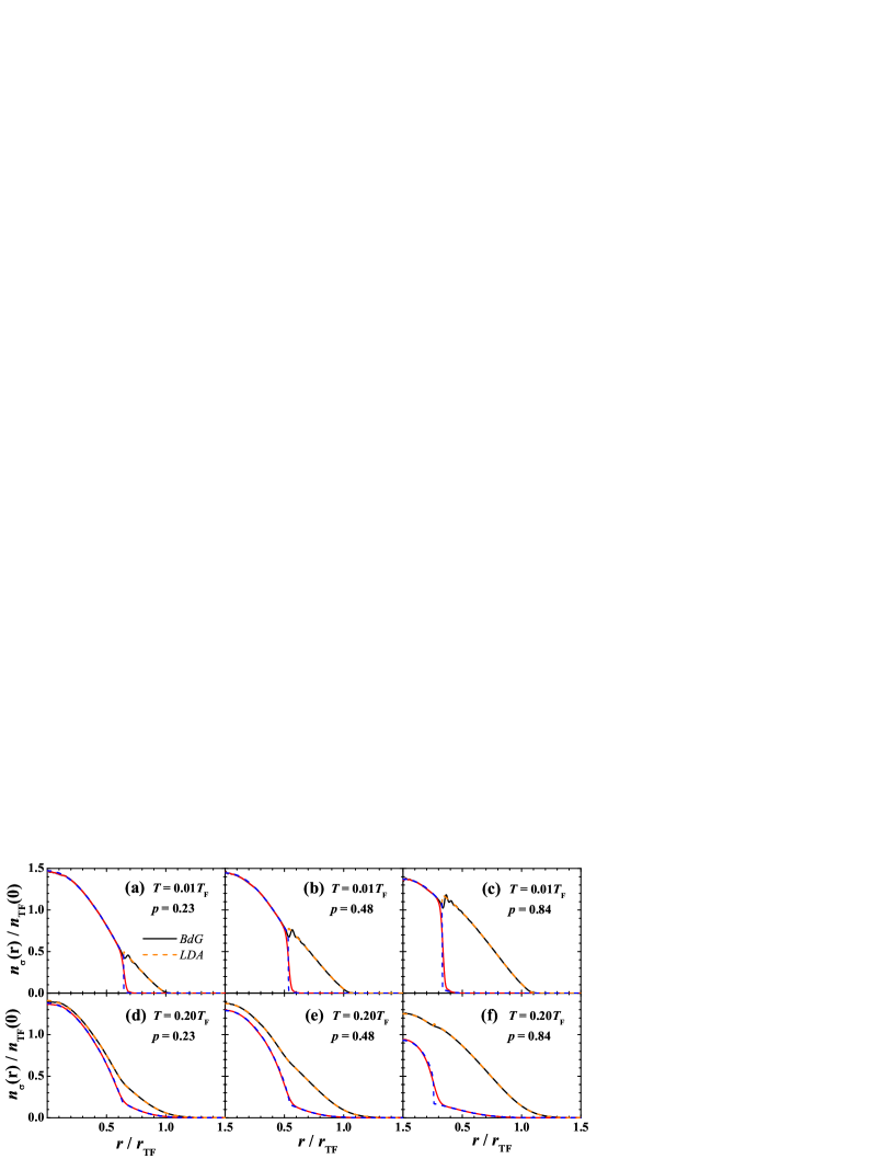
Figure 1: (color online). Density profiles of spin up and spin down atoms for a spin-polarized unitary Fermi gas at different population imbalances and temperatures, as indicated in the figures. The number of total atoms is $N=20000$. The density profiles are normalized by the Thomas-Fermi center density of an ideal symmetric Fermi gas with the same number of total atoms $n_{TF}(0)=\left(24N\right)^{1/2}a_{ho}^{-3}/\left(3\pi^{2}\right)$, while the length is renormalized by the corresponding Thomas-Fermi radius $r_{TF}=\left(24N\right)^{1/6}a_{ho}$. The solid lines and dashed lines refer to the BdG results and LDA results, respectively.

V.1 LDA versus BdG

We present in Fig. 1 the density profiles of two spin states at temperatures $T=0.01T_{F\text{ }}$ and $T=0.20T_{F\text{ }}$ for different population imbalances $P=\left(N_{\uparrow}-N_{\downarrow}\right)/\left(N_{\uparrow}+N_{\downarrow}\right)=0.23$, $0.48$ and $0.84$ as indicated. The results from the BdG and LDA approaches are plotted using solid lines and dashed lines, respectively. There is an apparent phase separation phenomenon, with a superfluid inner core and normal shell outside, which is in consistent with the recent experimental observation by Zwierlein et al. mit2006b and Partridge et al. rice . Particularly, for $P=0.84$ at $T=0.20T_{F\text{ }}$ the minority (spin down) profile is enhanced at center, which in turn induces a slight decrease of the central density of the majority component. The appearance of a dense central feature in the minority spin profile agrees well with the on-resonance measurement reported by Zwierlein et al. mit2006b . It clearly resembles the bimodal structure in the density distribution of a BEC.

For all the spin polarizations considered, we find reasonable agreement between these two methods at the chosen total number of atoms $N=20000$. As we shall see below, the agreement persists in various thermodynamical quantities, such as the chemical potential, entropy and total energy. >From the density profiles, the agreement is excellent at a small or intermediate population imbalance. The difference between the BdG and LDA prediction tends to be smaller as the temperature increases. For a large population imbalance, however, the agreement becomes worse. This can be understood from the corresponding gap functions as given in Fig. 2. The gap function in LDA experiences a sudden decrease at the superfluid-normal interface. With increasing population imbalance, the drop is much more apparent, and accordingly, the BdG gap function show a very pronounced oscillation behavior. Therefore, the deviation of the BdG density profiles from the LDA predictions becomes larger.

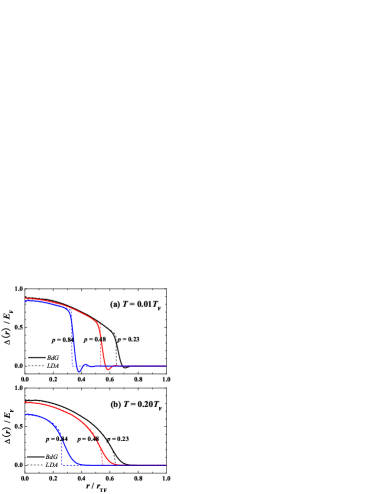
Figure 2: (color online). Gap functions at different temperatures $T=0.01T_{F}$ (a) and $T=0.20T_{F}$ (b) for various population imbalances as labeled. The number of total atoms is $N=20000$. The solid lines are the BdG predictions, while the dashed lines are the LDA results. The value of gap is renormalized by the non-interacting Fermi energy of an ideal symmetric Fermi gas $E_{F}=\left(3N\right)^{1/3}\hbar\omega$. Note that the small oscillation in the gap function at the superfluid-normal interface at low temperature $T=0.01T_{F}$ vanish when the temperature becomes high enough.

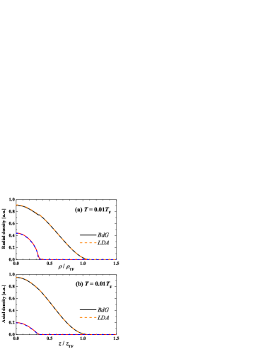
Figure 3: (color online). Radial (a) and axial (b) column density profiles for $N=20000$ and $P=0.84$ at $T=0.01T_{F}$. The difference between the BdG results (solid lines) and LDA results (dashed lines) becomes extremely small due to the integration over the extra dimensions.

It is important to note that only the axial column density or radial column density can be measured by the absorption imaging technique in the experiment. In Figs. 3a and 3b, we plot respectively the axial column profile and radial column profile at $T=0.01T_{F}$ for the imbalance $P=0.84$. The minor difference between BdG and LDA shown in the three-dimensional density profiles is essentially washed out.

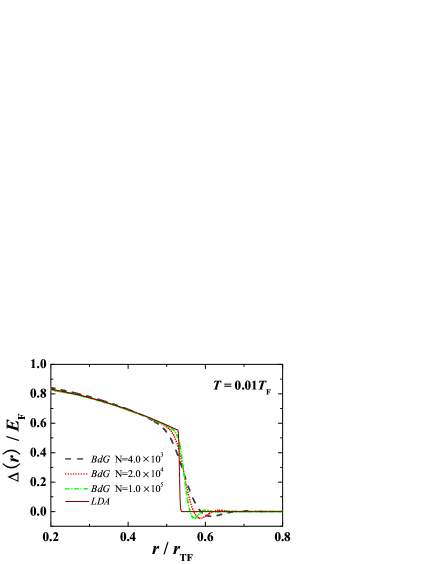
Figure 4: (color online). Dependence of the gap function on the number of total atoms at $T=0.01T_{F}$ and $P=0.48$. The solid line is the LDA result, and the others are BdG results with $N=10^{5}$ (dash-dotted line), $N=20000$ (dotted line), and $N=4000$ (dashed line).

V.2 FFLO state at the superfluid-normal interface?

The consistency between BdG and LDA treatments reported here is in sharp contrast with some previous studies castorina ; kinnunen ; machida ; jensen , where a notable discrepancy of BdG and LDA results is found. In those studies the small oscillation of the gap functions at the superfluid-normal interface is interpreted as the appearance of a spatially modulated FFLO state. Thus, the discrepancy is explained as due to the breakdown of LDA approximation for FFLO states. From our results, the oscillation in the order parameters at the interface appears to be a finite size effect. This idea is supported by the observation that the BdG formalism naturally reduces to that of LDA if we set the cut-off energy $E_{c}$ to zero as we mentioned earlier. On the other hand, as shown in Fig. 4, if we increase the number of total particles, the oscillation behavior of gap functions becomes gradually weaker. We thus infer that the oscillation will vanish finally in the limit of sufficient large number of atoms.

To understand the discrepancy of BdG and LDA approaches found in previous studies castorina ; kinnunen ; machida ; jensen , several remarks may be in order. First, in these studies, the mean-field Hartree terms, i.e., $Un_{\downarrow}\left({\bf r}\right)$ and $Un_{\uparrow}\left({\bf r}\right)$, appear in the decoupling of the interaction Hamiltonian in the BdG theory. However, the Hartree terms is absent in the corresponding LDA treatment. These terms cannot survive in the regularization procedure of the bare interaction $U$, but are incorrectly included in Refs. castorina ; kinnunen ; machida ; jensen as $\left(4\pi\hbar^{2}a/m\right)n_{\downarrow}\left({\bf r}\right)$ and $\left(4\pi\hbar^{2}a/m\right)n_{\uparrow}\left({\bf r}\right)$, respectively.

We note that the absence of the mean-field shift due to Hartree terms in the strongly interacting BCS-BEC crossover regime is already unambiguously demonstrated experimental by Gupta et al. mit2003 . We conclude that there are three main reasons for the differences between the conclusion we find here that the two approaches are compatible, as opposed to earlier conclusions to the contrary:

1. The incorrect inclusion of Hartree terms in one approach but not in the other, is the most likely reason for the discrepancy of BdG and LDA results shown in these previous works.

2. The accuracy of numerical results depends crucially on the regularization procedure used to treat the bare interaction $U$. Proper treatment of regularization is essential.

3. For a large population imbalance, the BdG equations converge very slowly. Thus, a rigorous criterion is required to ensure complete convergence.

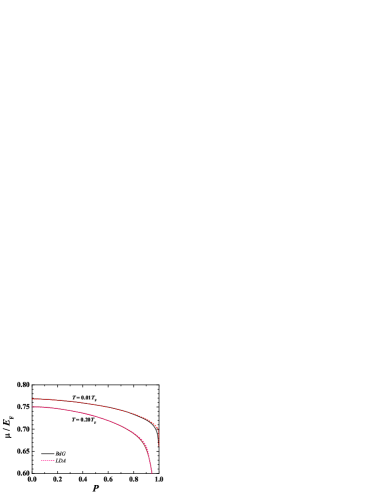
Figure 5: (color online). Chemical potentials as a function of the population imbalance at two temperatures $T=0.01T_{F}$ and $T=0.20T_{F}$.

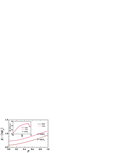
Figure 6: (color online). Total energy per particle as a function of the population imbalance $P$ at two temperatures $T=0.01T_{F}$ and $T=0.20T_{F}$. Inset shows the first order derivation with respect to the population imbalance at $T=0.20T_{F}$. The jump at $P\sim 0.9$ marks the phase transition to the normal state.

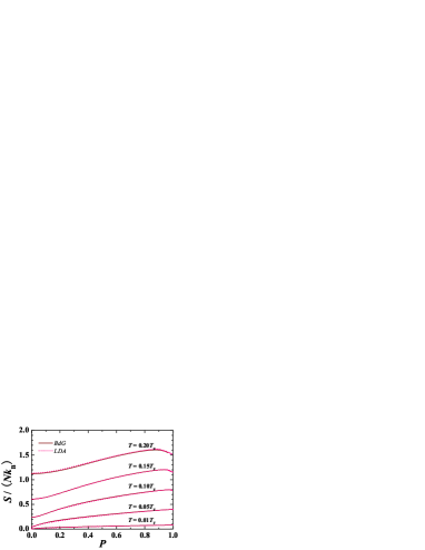
Figure 7: (color online). Entropy per particle as a function of the population imbalance at various temperatures.

V.3 Thermodynamic behavior of the imbalanced Fermi gas at unitarity

We finally discuss the thermodynamics of the gas at unitarity. In Figs. 5, 6, and 7, we graph the chemical potential, total energy and entropy of the gas as a function of the population imbalance at various temperatures. Again, we find good agreement between the BdG results and LDA predictions. With increasing population imbalance, the chemical potential decreases. For a given temperature there is a critical imbalance, beyond which the Fermi gas transforms into a fully normal state. The decrease of chemical potential becomes very significant when the phase transition occurs. In contrast, as population imbalance increases, the total energy increases. The impact of the phase transition on the total energy can scarcely be identified since the transition is smooth.

As shown in the inset of Fig. 6, it can be exhibited clearly in the first order derivative of the energy with respect to the population imbalance, resembling the behavior of the specific heat as a function of temperature. The entropy, on the other hand, shows a non-monotonic dependence at a temperature $\sim 0.20T_{F}$. We identify this peak position as the phase transition point.

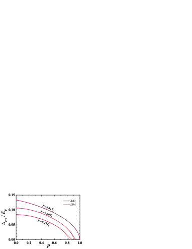
Figure 8: (color online). Average order parameter defined in Eq. (69) as a function of the population imbalance at three temperatures $T=0.01T_{F}$, $T=0.20T_{F}$, and $T=0.25T_{F}$. The position where the average order parameter vanishes determines the critical population imbalance towards the normal state at a fixed temperature.

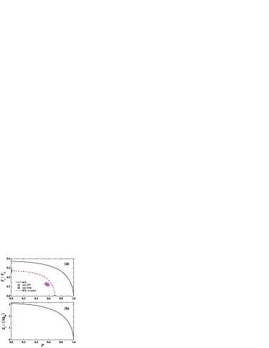
Figure 9: (color online). (a) BCS mean-field critical temperature as a function the population imbalance, determined from the LDA calculations (solid line). Open symbols are available experimental points from Zwierlein et al. mit2006b ; mit2006c and Kinast et al. duke2005 . The dashed line shows a re-scaled BCS critical temperature as described in the text. (b) The critical entropy (the entropy at the critical temperature) against the population imbalance.

To determine accurately the critical population imbalance as a function of temperature or vice versa, we plot in Fig. 8 an averaged order parameter at different temperature, which is defined via,

$$\Delta_{ave}=\left[\frac{\int_{0}^{\infty}dr4\pi r^{2}\Delta^{2}(r)}{N}\right]^{1/2}.$$ (69)

The condition $\Delta_{ave}=0$ therefore determines the critical population imbalance $P_{c}$ at a fixed temperature. The resulting $P_{c}$ from the BdG calculation depends, of course, on the number of total atoms. To remove this dependence, we present the LDA prediction for critical temperature in Fig. 9a. To compare with the experiments, we also show four known experimental points in the figure. The discrepancy between our theoretical predictions and the experimental data is most likely attributed to the strong pair fluctuations beyond the mean-field, i.e., for a symmetric gas, the fluctuation shifts $T_{c,BCS}$ from $0.37T_{F}$ to around $0.27T_{F}$ duke2005 , while at zero temperature, it reduce $P_{c,BCS}$ from $1.0$ to about $0.70$ mit2006a ; mit2006b .

Pair fluctuations must be taken into account in the strongly interacting unitarity regime for quantitative comparisons, as we have shown in earlier calculations hld without spin-polarization. This is certainly the most challenging problem in BCS-BEC crossover physics. Naively, we may linearly rescale the BCS critical temperature and population imbalance in such a way that both the theoretical $T_{c}$ at $P=0$ and $P_{c}$ at $T=0$ fits the experimental data. The third and fourth experimental points of critical temperature at $P=0.56(3)$ and $P=0.59(3)$ now agree approximately with the re-scaled BCS $T_{c}$ curve.

For strongly interacting Fermi gases at low temperature, there is generally no reliable thermometry technique. The bimodal structure in the density profile of the minority component may provide a useful method to determine temperature mit2006b . However its accuracy requires further theoretical investigations due to the strongly correlated nature of the gas. Entropy is an alternative quantity that may be used to characterize the temperature in adiabatic passage experiments hldT . In Fig. 9b, we show also the critical entropy of a trapped unitary gas against the population imbalance. The calculated dependence is essentially similar to that for temperature.

VI Conclusions

We have developed an efficient and accurate hybrid procedure to solve the mean-field BdG equations for a spherically trapped Fermi gas with spin population imbalance. This enables us to thoroughly examine the extensively used LDA approach. For a moderate large particle number ($\sim 10^{4}$), the LDA appears to work very well. The discrepancy of BdG and LDA results reported in previous studies is attributed to the incorrect inclusion of a mean-field Hartree term in the BdG equations. We note, however, that the trap used in the current experiments is elongated in the axial direction. The spherical trap considered in this work may be regarded as approximately representative of the experimental setup by Zwierlein et al. mit2006a ; mit2006b ; mit2006c with an aspect ratio approximately 5. The trap in the experiment by Partridge et al. rice is extremely anisotropic, and therefore the LDA description could break down. The solution of the BdG equations for such elongated systems is numerically intensive, and requires further investigation.

Our derivation of the BdG formalism and the numerical results with varying particle number in Fig. 4 strongly suggest that the calculated small oscillation in the order parameter at the superfluid-normal interface arises from finite size effects. This is in marked contrast with the previous interpretation of this effect as due to a finite-momentum paired FFLO state castorina ; kinnunen ; machida ; jensen . The detailed structure of the proposed FFLO state is not clear, even in the homogeneous situation. How to extend the current BdG formalism to incorporate the FFLO state is therefore a fascinating issue. Another possibility is that the extremely narrow window for FFLO states in 3D is closed or reduced in size due to the presence of the harmonic trap.

We have reported various mean-field thermodynamical properties of the imbalanced Fermi gas at unitarity, which is believed to be qualitatively reliable at low temperature. The experimentally observed bimodal distribution in the profile of the minority spin state has been reproduced. We have determined the BCS superfluid transition temperature as a function of the population imbalance, and have shown that it is consistent with recent experimental measurements. Quantitative theories of the imbalanced Fermi gas that take account of large quantum fluctuations that occur in the strongly correlated unitarity regime still need to be developed. A promising approach is to take into account pair fluctuations within the ladder approximation hld . This problem will be addressed in a future publication.

- (1) C. A. Regal and D. S. Jin, Phys. Rev. Lett. 92, 040403 (2004).
- (2) M. W. Zwierlein et al., Phys. Rev. Lett. 92, 120403 (2004).
- (3) J. Kinast et al., Phys. Rev. Lett. 92, 150402 (2004).
- (4) M. Bartenstein et al., Phys. Rev. Lett. 92, 203201 (2004).
- (5) H. Hu et al., Phys. Rev. Lett. 93, 190403 (2004).
- (6) C. Chin et al., Science 305, 1128 (2004).
- (7) J. Kinast et al., Science 307, 1296 (2005).
- (8) M. W. Zwierlein et al., Nature (London) 435, 1047 (2005).
- (9) M. W. Zwierlein et al., Science 311, 492 (2006).
- (10) M. W. Zwierlein et al., Nature (London) 442, 54 (2006)
- (11) Y. Shin et al., Phys. Rev. Lett. 97, 030401 (2006).
- (12) G. B. Partridge et al., Science 311, 503 (2006).
- (13) P. Fulde and R. A. Ferrell, Phys. Rev. 135, A550 (1964); A. I. Larkin and Y. N. Ovchinnikov. Zh. Eksp. Teor. Fiz. 47, 1136 (1964) [Sov. Phys. JETP 20, 762 (1965)].
- (14) W. V. Liu and F. Wilczek, Phys. Rev. Lett. 90, 047002 (2003).
- (15) G. Sarma, J. Phys. Chem. Solids 24, 1029 (1963).
- (16) S.-T. Wu and S.-K. Yip, Phys. Rev. A 67, 053603 (2003).
- (17) C.-H. Pao, S.-T. Wu, and S.-K. Yip, Phys. Rev. B. 71, 132506 (2006).
- (18) P. F. Bedaque, H. Caldas, and G. Rupak, Phys. Rev. Lett. 91, 247002 (2003).
- (19) D. T. Son and M. A. Stephanov, Phys. Rev. A 74, 013614 (2006).
- (20) K. Yang, cond-mat/0508484; cond-mat/0603190.
- (21) D. E. Sheehy and L. Radzihovsky, Phys. Rev. Lett. 96, 060401 (2006); cond-mat/0607803.
- (22) H. Hu and X.-J. Liu, Phys. Rev. A 73, 051603(R) (2006).
- (23) X.-J. Liu and H. Hu, Europhys. Lett. 75, 364 (2006).
- (24) A. Bulgac, M. M. Forbes, and A. Schwenk, Phys. Rev. Lett. 97, 020402 (2006)).
- (25) M. Mannarelli, G. Nardulli, and M. Ruggieri, Phys. Rev. A 74, 033606 (2006).
- (26) C.-C. Chien, Q. Chen, Y. He, and K. Levin, Phys. Rev. Lett. 97, 090402 (2006).
- (27) M. M. Parish et al., cond-mat/0605744.
- (28) R. Casalbuoni and G. Nardulli, Rev. Mod. Phys. 76, 263 (2004).
- (29) H. Müther and A. Sedrakian, Phys. Rev. Lett. 88, 252503 (2002); A. Sedrakian et al., Phys. Rev. A 72, 013613 (2005); A. Sedrakian, H. Müther and, and A. Polls, Phys. Rev. Lett. 97, 140404 (2006).
- (30) J. Carlson and S. Reddy, Phys. Rev. Lett. 95, 060401 (2005).
- (31) L. He, M. Jin, and P. Zhang, Phys. Rev. B 73, 214527 (2006).
- (32) H. Caldas, cond-mat/0601148; cond-mat/0605005.
- (33) T.-L. Ho and H. Zhai, cond-mat/0602568.
- (34) Z.-C. Gu, G. Warner, and F. Zhou, cond-mat/0603091.
- (35) M. Iskin and C. A. R. Sá de Melo, Phys. Rev. Lett. 97, 100404 (2006).
- (36) S.-T. Wu, C.-H. Pao, and S.-K. Yip, cond-mat/0604572.
- (37) F. Chevy, Phys. Rev. Lett. 96, 130401 (2006); cond-mat/0605751.
- (38) W. Yi and L.-M. Duan, Phys. Rev. A 73, 031604 (2006); Phys. Rev. A. 74, 013610 (2006).
- (39) T. N. De Silva and E. J. Mueller, Phys. Rev. A 73, 051602(R) (2006); Phys. Rev. Lett. 97, 070402 (2006).
- (40) M. Haquea and H. T. C. Stoof, Phys. Rev. A 74, 011602(R) (2006).
- (41) C.-H. Pao and S.-K. Yip, J. Phys.: Condensed Matter 18, 5567 (2006);
- (42) A. Imambekov et al., cond-mat/0604423.
- (43) J.-P. Martikainen, Phys. Rev. A 74, 013602 (2006).
- (44) C.-C. Chien, Q. Chen, Y. He, and K. Levin, Phys. Rev. A 74, 021602(R) (2006).
- (45) A. Bulgac and M. M. Forbes, cond-mat/0606043.
- (46) K. B. Gubbels, M. W. J. Romanns, and H. T. C. Stoof, cond-mat/0606330.
- (47) T. Mizushima, K. Machida, and M. Ichioka, Phys. Rev. Lett. 94, 060404 (2005).
- (48) P. Castorina et al., Phys. Rev. A 72, 025601 (2005).
- (49) J. Kinnunen, L. M. Jensen, and P. Törm? Phys. Rev. Lett. 96, 110403 (2006).
- (50) K. Machida, T. Mizushima, and M. Ichioka, Phys. Rev. Lett. 97, 120407 (2006).
- (51) L. M. Jensen, J. Kinnunen, and P. Törm? cond-mat/0604424.
- (52) T.-L. Ho, Phys. Rev. Lett. 92, 090402 (2004).
- (53) S. Gupta et al., Science 300, 1723 (2003).
- (54) K. V. Kheruntsyan and P. D. Drummond, Phys. Rev. A 61, 063816 (2000); S. J. J. M. F. Kokkelmans et al., Phys. Rev. A 65, 053617 (2002); P. D. Drummond and K. V. Kheruntsyan, Phys. Rev. A 70, 033609 (2004).
- (55) G. B. Partridge et al., Phys. Rev. Lett. 95, 020404 (2005).
- (56) R. Diener and T.-L. Ho, cond-mat/0405174.
- (57) X.-J. Liu and H. Hu, Phys. Rev A 72, 063613 (2005).
- (58) Henning Heiselberg, Phys. Rev A 63, 043606 (2001).
- (59) P. de Gennes, Superconductivity of Metals and Alloys (Addison-Wesley, New York, 1966).
- (60) J. Reidl et al., Phys. Rev. A 59, 3816 (1999).
- (61) G. Bruun et al., Eur. Phys. J. D 7, 433 (1999).
- (62) A. Bulgac and Y. Yu, Phys. Rev. Lett. 88, 042504 (2002).
- (63) M. Grasso and M. Urban, Phys. Rev. A 68, 033610 (2003).
- (64) H. Hu, X.-J. Liu, and P. D. Drummond, Europhys. Lett. 74, 574 (2006).
- (65) H. Hu, X.-J. Liu, and P. D. Drummond, Phys. Rev. A 73, 023617 (2006).