Signatures of Discontinuity in the Exchange-Correlation Energy Functional Derived from the Subband Electronic Structure of Semiconductor Quantum Wells

Abstract

The discontinuous character of the exact exchange-correlation $(xc)$ energy functional of Density Functional Theory is shown to arise naturally in the subband spectra of semiconductor quantum wells. Using an ab-initio $xc$ functional, including exchange exactly and correlation in an exact partial way, a discontinuity appears in the $xc$ potential, each time a subband becomes slightly occupied. Exchange and correlation give opposite contributions to the discontinuity, with correlation overcoming exchange. The jump in the intersubband energy is in excellent agreement with experimental data.

Density Functional Theory (DFT) has become the standard calculational tool in physics and quantum chemistry for the study of atomic, molecular, and solid state systems. The theory is based in the Hohenberg-Kohn theoremsparr , that place the ground-state electron density as the basic variable and provides a variational principle for its calculation. Kohn and Sham (KS) showed how the problem of variational minimization for the density could be exactly mapped to one of non-interacting particles in an effective potential, which contains only one non-trivial component: the exchange-correlation ($xc$) contributionparr . DFT, however, gives no clue on how to proceed for its practical calculation. Naturally a lot of attention has been devoted to the development of better $xc$ energy functionals; KS introduced the highly successful Local Density Approximation (LDA), which is widely employed nowadays, along with the improvements born from it (such as the Generalized Gradient Approximation or GGA, meta-GGA, etc.)tao . The work described here is motivated by this fundamental need of better approximations for the $xc$ energy functionalmattsson , using as "laboratory" to test the accuracy of the approximations the subband electronic structure of the quasi two-dimensional electron gases (2DEG) formed at the interface between two dissimilar semiconductors, such as GaAs and AlGaAs. In this Letter we show that at the one-subband $\rightarrow$ two-subband quantum well (QW) transition ($1S\rightarrow 2S$), the $xc$ potential behaves discontinuously, with exchange and correlation giving opposite contributions (i.e., competing) to the discontinuity. The intersubband energy, which also jumps abruptly at the transition, is in excellent agreement with experiments.

Our model system is a semiconductor modulation-doped QW grown epitaxially, as shown in the upper inset of Fig. 1. Assuming translational symmetry in the $(x-y)$ plane (area $A$), and proposing accordingly a solution of the type $\phi_{i\mathbf{k}\sigma}(\mbox{\boldmath$\rho$},z)=\text{e}^{i\mathbf{k}\cdot\mbox{\boldmath$\rho$}}\xi_{i}^{\sigma}(z)/\sqrt{A}$, with $\rho$ the in-plane coordinate, the zero temperature ground-state electron density can be obtained by solving a set of effective one-dimensional KS equations of the form:

$$\left[-\frac{1}{2}\frac{\partial^{2}}{\partial z^{2}}+V_{KS}^{\sigma}(z)\right]\xi_{i}^{\sigma}(z)=\varepsilon_{i}^{\sigma}\xi_{i}^{\sigma}(z),$$ (1)

where effective atomic units have been used. $\xi_{i}^{\sigma}(z)$ is the wavefunction for electrons in subband $i$ ($i=1,\,2,\,...$), spin $\sigma$ ($\sigma=\uparrow,\,\downarrow$), and eigenvalue $\varepsilon_{i}^{\sigma}$. The local (multiplicative) KS potential $V_{KS}^{\sigma}(z)$ is the sum of several terms: $V_{KS}^{\sigma}(z)=V_{ext}(z)+V_{H}(z)+V_{xc}^{\sigma}(z)$. $V_{ext}(z)$ is given by the epitaxial potential plus an external electric field. $V_{H}(z)$ is the Hartree potential. Within DFT, $V_{xc}^{\sigma}(z)=A^{-1}\delta E_{xc}/\delta n_{\sigma}(z)$. Departing from the main stream in most applications of KS-DFT, our $xc$ energy functional is an explicit functional of the whole set of $\varepsilon_{i}^{\sigma}$’s and $\xi_{i}^{\sigma}$’s, $E_{xc}=E_{xc}[\{\varepsilon_{i}^{\sigma},\xi_{i}^{\sigma}\}]$, but an implicit (in general unknown) functional of the spin-resolved density $n_{\sigma}(z)$. The zero-temperature $3D$ electron density is $n_{\sigma}(z)=\sum_{\varepsilon_{i}^{\sigma}<\mu}(\mu-\varepsilon_{i}^{\sigma})|\xi_{i}^{\sigma}(z)|^{2}/2\pi$, with $\mu$ the chemical potential. By assuming a paramagnetic situation, we drop the spin index $\sigma$ from this point.

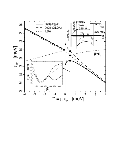
Figure 1: Ground-state $\rightarrow$ first-excited intersubband energy $\varepsilon_{12}$ as a function of $\Gamma$. Negative (positive) values of $\Gamma$ correspond to the $1S$ ($2S$) regime. Upper inset: schematic view of our model for the modulation-doped QW. A charge-transfer field along $z$ is induced by a distant metallic plate (thin vertical line at right). If the metallic plate is positively (negatively) charged, more (less) electrons are transferred towards the well from an ionized donor impurities region (thick vertical stripe at left), which acts as a particle reservoir fixing the chemical potential $\mu$. Lower inset: $V_{xc}(z)$ in the same three different approximations as for $\varepsilon_{12}$ ($\Gamma=0.5$ meV) . The QW extends from $z=50$ Å   to $z=295$ Å.

The $xc$ energy functional $E_{xc}$ for our 2DEG has been generated by Görling-Levy (GL) perturbation theory where the correlation energy is expanded in a seriesgorling ,

$$E_{xc}[\{\varepsilon_{i},\xi_{i}\}]=E_{x}[\{\varepsilon_{i},\xi_{i}\}]+\sum_{n=2}^{\infty}E_{c}^{GL(n)}[\{\varepsilon_{i},\xi_{i}\}],$$ (2)

which is truncated at its leading contribution $n=2$. $E_{x}$ in equation above is the exact exchange energy, known explicitly as a Fock integral of the KS occupied orbitals. Its multi-subband explicit expression is given by Eq.(38) in Ref.rigamonti1 (denoted as I below). The terms $E_{c}^{GL(n)}$ can be found explicitlygorling . At difference with $E_{x}$, however, they depend both on occupied and an infinite number of unoccupied subbands. Their numerical evaluation is in consequence rather expensive. The explicit expression for $E_{c}^{GL(2)}$ for our semiconductor QW system is given by Eqs.(32) and (33) of I. A similar correlation energy functional has been used in Refs.mori and jiang for the case of atoms, with mixed results. As shown here, Eq.(2) seems much more promising for the 2DEGnote .

The next non-trivial problem is the evaluation of $V_{xc}(z)$, given the already quoted implicit dependence of $E_{xc}$ on $n(z)$ in Eq. (2). The procedure for dealing with implicit functionals relies on the use of the chain rule for functional derivatives as follows gorling :

$$V_{xc}(z)=\frac{1}{A}\frac{\delta E_{xc}}{\delta n(z)}=\frac{1}{A}\int\frac{\delta E_{xc}}{\delta V_{KS}(z^{\prime})}\frac{\delta V_{KS}(z^{\prime})}{\delta n(z)}dz^{\prime}.$$ (3)

To proceed with the calculation of $V_{xc}(z)$ directly from Eq.(3), we use a numerical method devised and explained in detail in I. Eqs.(1)-(3) should be iterated until full self-consistency is achieved.

We present in Fig. 1 the intersubband energy spacing $\varepsilon_{12}\equiv\varepsilon_{2}-\varepsilon_{1}$, as a function of $\Gamma\equiv\mu-\varepsilon_{2}$, for three approximations for $E_{xc}$: LDA, exact-exchange plus LDA for correlation [X(X)-C(LDA)], and X(X) plus partial exact-correlation ($E_{c}^{GL(2)}$), denoted as X(X)-C(pX). Note that while the resulting $\varepsilon_{12}$ are quite similar in the three approximations in the whole $1S$ regime, and in the $2S$ regime with sizable occupation of the second subband, noticeable differences arise in the limit of small second subband occupancy. Starting with the X(X)-C(LDA) approximation, $\varepsilon_{12}$ shows an exchange-driven abrupt positive jump at the $1S\rightarrow 2S$rigamonti2 . The inclusion of C(pX) overcomes the X(X)-C(LDA) positive jump, resulting now in a negative jump in $\varepsilon_{12}$, until it levels with the other results at finite second subband fillings. LDA is in between the two kind of discontinuities at $\Gamma=0$, showing only a discontinuity in the derivative. The lower inset shows the corresponding $V_{xc}(z)$ in the relevant QW region. $V_{xc}(z)$ as resulting from X(X)-C(LDA) builds a barrier just where most of the weight of $\xi_{2}(z)$ is concentrated, pushing $\varepsilon_{2}$ upwards under small occupancy of the second subband, and leaving $\varepsilon_{1}$ more or less unaltered; this explains the discontinuous positive behavior of $\varepsilon_{12}$. It is also physically reasonable: by blocking the occupation of the second subband, the exchange energy is optimized, as the intrasubband exchange is larger than the intersubband exchange. The $V_{xc}(z)$ in the X(X)-C(pX) behaves just in the opposite way: it develops a deep well just after the transition, inducing an abrupt decrease of $\varepsilon_{2}$ at more or less constant $\varepsilon_{1}$. This explains the abrupt decrease of $\varepsilon_{12}$ in this case. The behavior has again a simple physical explanation: by inducing the occupancy of the second subband, $V_{xc}(z)$ promotes a spatial separation between electrons in both subbands, decreasing correlation and its associated repulsive energy. With respect to the $V_{xc}(z)$ resulting from LDA, it shows the expected smooth and continuous behavior at the transition.

Besides these fully numerical results, we provide below an analytical derivation of the results of Fig. 1, for $\Gamma\simeq 0$. In the limit $|\Gamma|\rightarrow 0$, $E_{xc}$ can be approximated as

$$E_{xc}^{(\alpha)}=P_{xc}^{(\alpha)}+\Gamma Q_{xc}^{(\alpha)},$$ (4)

with $\alpha=1S,2S$. Here, $P_{xc}^{(1S)}=E_{xc}(\Gamma\rightarrow 0^{-})$, $P_{xc}^{(2S)}=E_{xc}(\Gamma\rightarrow 0^{+})$, $Q_{xc}^{(1S)}=dE_{xc}/d\Gamma|_{0^{-}}$, $Q_{xc}^{(2S)}=dE_{xc}/d\Gamma|_{0^{+}}$. By inspection of the explicit expressions for $E_{x}$ and $E_{c}^{GL(2)}$ given in I, it is concluded that $P_{xc}^{(1S)}=P_{xc}^{(2S)}=P_{xc}$, and that $Q_{xc}^{(1S)}\neq Q_{xc}^{(2S)}$. In words, for a fixed set of $\varepsilon_{i\neq 2}$’s and $\xi_{i}(z)$’s, the $xc$ functional is continuous at the $1S\rightarrow 2S$, but its derivative is discontinuous. The explicit expressions for $P_{xc}$, $Q_{xc}^{(1S)}$ and $Q_{xc}^{(2S)}$ are not needed for the present derivation. Inserting Eq.(4) in Eq.(3) we obtain,

$$V_{xc}^{(\alpha)}(z)\!=\!\!\!\int\!\!\left[\!\frac{\delta P_{xc}}{\delta V_{KS}(z^{\prime})}\!-\!Q_{xc}^{(\alpha)}|\xi_{2}(z^{\prime})|^{2}\right]\!\chi_{\alpha}^{-1}(z^{\prime},z)dz^{\prime}.$$ (5)

Here, we have defined $\chi_{\alpha}^{-1}(z,z^{\prime})\equiv\delta V_{KS}(z)/\delta n_{\alpha}(z^{\prime})$, and used the result $\delta\Gamma/\delta V_{KS}(z)=-\delta\varepsilon_{2}/\delta V_{KS}(z)=-|\xi_{2}(z)|^{2}$, obtained by first-order perturbation theory. We have also neglected a term lineal in $\Gamma$, which becomes arbitrarily small in the limit $\Gamma\rightarrow 0$. In the limit $\Gamma\rightarrow 0^{+}$, the density response functionrigamonti1 becomes

$$\chi_{2S}(z,z^{\prime})=\chi_{1S}(z,z^{\prime})-\left|\xi_{2}(z)\xi_{2}(z^{\prime})\right|^{2}/\pi.$$ (6)

Its inverse can be calculated by using the Sherman-Morrison techniquenumrec . We obtain

$$\chi_{2S}^{-1}(z,z^{\prime})=\chi_{1S}^{-1}(z,z^{\prime})+D(z)D(z^{\prime})/[\pi(1+\lambda)],$$ (7)

where $D(z)=\int\chi_{1S}^{-1}(z,x)|\xi_{2}(x)|^{2}dx$, and $\lambda=-\pi^{-1}\int D(x)|\xi_{2}(x)|^{2}dx$. As we can see from Eq.(7), $\chi_{2S}^{-1}(z,z^{\prime})$ is discontinuous at the $1S\rightarrow 2S$ transition, such as it is $\chi_{2S}(z,z^{\prime})$ of Eq.(6). Using now Eq.(5) for $\alpha=1S,2S$ and exploiting the explicit expression for $\chi_{2S}^{-1}(z,z^{\prime})$ as given by Eq.(7), we arrive at the result

$$\Delta V_{xc}(z)\equiv V_{xc}^{(2S)}(z)-V_{xc}^{(1S)}(z)=C_{xc}D(z)/(1+\lambda),$$ (8)

with $C_{xc}=\langle V_{xc}^{(1S)}\rangle_{2}/\pi-\Delta Q_{xc}$, $\left\langle{\cal O}\right\rangle_{i}=\int dx|\xi_{i}(x)|^{2}{\cal O}(x)$ and $\Delta Q_{xc}=Q_{xc}^{(2S)}-Q_{xc}^{(1S)}$. Eq.(8) is an important result, which shows explicitly how the functional dependence on $z$ of the $xc$ potential changes discontinuously at the $1S\rightarrow 2S$ transition. For an arbitrary subband transition $NS\rightarrow(N+1)S$ it can be shown that the result of Eq.(8) is still valid, with the replacements $1\rightarrow N$ and $2\rightarrow N+1$ in Eqs.(4)-(8). Equation 8 follows rigorously from Eq.(4), and then it is important to discuss its validity. In writing Eq.(4) we have implicitly made a "frozen" assumption, by taking the same set of wavefunctions $\xi_{i}(z)$ and energies $\varepsilon_{i}$ both for $\Gamma\rightarrow 0^{-}$ and $\Gamma\rightarrow 0^{+}$. In the language of the numerical self-consistent calculations leading to Fig. 1, it is as if the results for the $1S$ case in the limit $\Gamma\rightarrow 0^{-}$ were extrapolated to the $2S$ $\Gamma\rightarrow 0^{+}$ case, by performing a single iteration loop towards full self-consistency. This "frozen" result for the $xc$ energy functional is illustrated in Fig. 2 by the straight lines, separating exchange ($P_{x}+\Gamma Q_{x}^{\alpha}$) from correlation ($P_{c}+\Gamma Q_{c}^{\alpha}$). Besides, if the approximation for $E_{xc}$ is such that $\Delta V_{xc}(z)\neq 0$ (that is, if $C_{xc}\neq 0$), it is clear that the self-consistent iteration loop will lead to a further discontinuity in the $xc$ energy functional itself right at the $1S\rightarrow 2S$ transition $(\Gamma=0)$, once convergence has been reached. These fully self-consistent results correspond to the thick full ($E_{x}$) and dashed ($E_{c}^{GL(2)}$) lines in Fig. 2. On the other side, if the approximation for $E_{xc}$ is such that $C_{xc}=0$, no discontinuity of the type of Eq.(8) exists for $V_{xc}(z)$ before or after self-consistency is achieved, which in turn implies the continuity of $E_{xc}$. Our $E_{xc}=E_{xc}[\{\varepsilon_{i}^{\sigma},\xi_{i}^{\sigma}\}]$ is such that $C_{xc}\neq 0$; local (LDA) approximations for $E_{xc}$ yield $C_{xc}=0$.

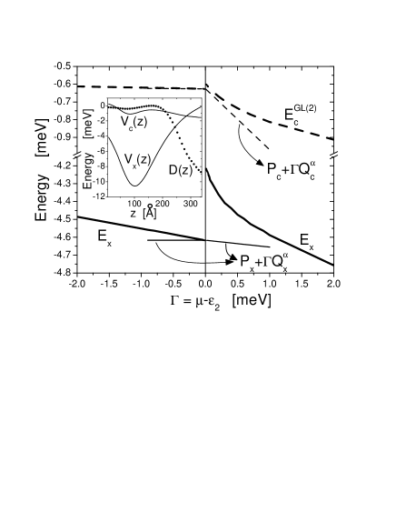
Figure 2: Full lines: $E_{x}$ in the "frozen" (thin line) and self-consistent (thick line) approaches; dashed lines: $E_{c}^{GL(2)}$ in the "frozen" (thin line) and self-consistent (thick line) approaches. Note the cut in the vertical scale. Inset: exchange and correlation potentials (full lines) and function $D(z)$ (dotted line, arbitrary units) for $\Gamma=-\hskip 2.0pt0.01$ meV.

For further insight, the constant $C_{xc}$ can be separated conveniently in its exchange and correlation components $C_{n}=\langle V_{n}^{(1S)}\rangle_{2}/\pi-\Delta Q_{n}$, with $n=x,c$. The analysis of the results shown in Fig. 2 leads to the conclusion that $C_{x}<0$ and $C_{c}>0$, considering that $D(z)<0$ (see inset in Fig. 2). Qualitatively, this happens in the following way: a) in the exchange case, $\langle V_{x}^{(1S)}\rangle_{2}$ is large and negative (see inset Fig. 2), while $-\Delta Q_{x}$ is a relatively small positive magnitude, resulting in $C_{x}<0$; b) in the correlation case, $\langle V_{c}^{(1S)}\rangle_{2}$ is a very small quantity (see inset Fig. 2), while $-\Delta Q_{c}$ is a relatively large positive number, yielding a $C_{c}>0$. The net result is that correlation overcomes exchange ($C_{xc}=C_{x}+C_{c}>0$), and $\Delta V_{xc}(z)$ has a negative contribution resulting in the right attractive well shown in the lower inset of Fig. 1. It is important to note that this overcoming of correlation on exchange happens even when $|E_{c}^{GL(2)}|\ll|E_{x}|$ (Fig. 2). However, as Eq.(8) clearly shows, not only the magnitude of the $xc$ energy functional matters (represented by the $\langle V_{xc}^{(1S)}\rangle_{2}$ contribution), but also the respective derivatives (represented by the $\Delta Q_{xc}$ term). This exemplifies quite vividly the potential danger of neglecting correlation against exchange at the threshold of a subband transition, under the argument that the correlation energy is much smaller than the exchange energy.

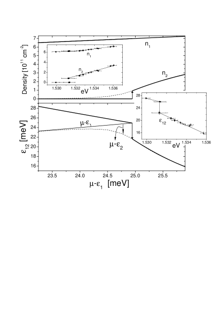
Figure 3: Thick full lines: Ground and first-excited subband densities $n_{1}$ and $n_{2}$ (upper panel) and intersubband transition energy $\varepsilon_{12}$ (lower panel) as a function of $\mu-\varepsilon_{1}$. Dashed lines: $n_{2}$ and $\varepsilon_{12}$ corresponding to a continuous filling of the first-excited subband, as in Fig. 1. Insets: experimental data from Ref.[goni, ].

Is there any experimental evidence of this type of discontinuities in semiconductor QW’s? The answer is yes. We reproduce as an inset in the upper panel of Fig. 3 the experimental values for the subband densities $n_{1}$ and $n_{2}$, plotted as a function of the Fermi level measured from the top of the valence bandgoni . The data have been obtained from a quantitative analysis of photoluminescence line shapes. It is seen that when the Fermi level touches the bottom of the second subband, the electron density $n_{2}$ jumps from zero to a finite value ranging from $3\times$ 10¹⁰ to 8 $\times$ 10¹⁰ cm^-2, depending on temperaturegoni . The electron density of the lowest subband, in contrast, increases slightly but smoothly with voltage, suggesting that the external electric field couples essentially to the $1S$ occupation, which seems quite plausible as it is the subband with the largest occupation. This motivates us to redraw the results for $\varepsilon_{12}$ of Fig. 1 as a function of $\mu-\varepsilon_{1}$, in the lower panel of Fig. 3. Clearly the theoretical $n_{1}$, $n_{2}$, and $\varepsilon_{12}$ vs. $\mu-\varepsilon_{1}$ agree quite well with the experimental data, both qualitatively and quantitatively. For instance, the theoretical value for the decreasing jump in $\varepsilon_{12}$ at $\mu-\varepsilon_{1}\simeq$ 25 meV, amounts to about 3.3 meV, in excellent agreement with the 3.5 meV jump estimated from experiment.

The results presented in this work are intimately related to the issue of the derivative discontinuity of ensemble DFTperdew1 . Among the many important consequences derived from this extension of DFT to fractional particle number, maybe the most important one in the field of solid state physics has been the realization that the true gap of semiconductors is not given by the KS one-particle gapperdew2 . Instead, the true gap is given by the sum of the KS gap, plus the so-called $xc$ discontinuity, $\Delta_{xc}$. Continuum approximations to $xc$ energy functionals, including all currently widely used LDA’s and GGA’s, fail to produce the correct value for $\Delta_{xc}$, resulting in an important underestimation of the fundamental band-gap of most semiconductors and insulators. In a very recent work, Grüning et al. have clarified the theoretical situation, obtaining very good agreement between experimental and theoretical band gaps of Si, LiF, and Argruning , by using an orbital based correlation energy functional corresponding to a dynamical screening of the Coulomb interaction (GW approximation). It was found that $\Delta_{xc}$ contributes as much as $30\%-50\%$ to the energy gap. Their results, for a different type of systems, are fully consistent with ours.

In conclusion, the intrinsic discontinuity of the $xc$ energy functional has been obtained entirely within a DFT framework, for a realistic system. We have shown that the $xc$ energy functional generated by second-order Görling-Levy perturbation theory for the 2DEG has many of the properties of the exact functional. The main finding is that at the $1S\rightarrow 2S$ transition, the KS $xc$ potential and the associated intersubband transition energies behave discontinuously, with $x$ and $c$ giving opposite contributions (i.e. competing) to the discontinuity, and with correlation overcoming exchange. Very good qualitative and quantitative agreement is obtained with experiments.

This work was partially supported by CONICET under grant PIP 5254 and the ANPCyT under PICT 03-12742. SR acknowledges financial support from CNEA-CONICET. CRP is a fellow of CONICET.

References

- (1) R. G. Parr and W. Yang, Density Functional Theory of Atoms and Molecules, (Oxford University Press, New York, 1989); R. M. Dreizler and E. K. U. Gross, Density Functional Theory (Springer-Verlag, Heidelberg, 1990).
- (2) J. Tao et al., Phys. Rev. Lett. 91, 146401 (2003).
- (3) A. E. Mattsson, Science 298, 759 (2002).
- (4) A. Görling and M. Levy, Phys. Rev. B 47, 13105 (1993); ibid, Phys. Rev. A 52, 4493 (1995).
- (5) S. Rigamonti and C. R. Proetto, Phys. Rev. B 73, 235319 (2006). As the calculations of this work were restricted to the simpler regime, none of the findings of the present work concerning the transition were considered. There is also an important difference from the technical point of view: the calculation of in a situation with two (or more) occupied subbands is far more complicated and numerically demanding than the case, due to the presence in the many-subband case of four Fermi disk intersecting integrals, whose numerical evaluation becomes quite involved.
- (6) P. Mori-Sánchez, Q. Wu, and W. Yang, J. Chem. Phys. 123, 062204 (2005).
- (7) H. Jiang and E. Engel, J. Chem. Phys. 123, 224102 (2005).
- (8) As is well known, diverges in the long-wavelength limit for the case of the homogeneous 3D electron gaspines . In contrast, this contribution is finite for the strict 2D homogeneous electron gasrajagopal . Our QW system is much closer to the 2D than to the 3D limit (corresponding to a very large number of occupied subbands). It seems then quite plausible that the perturbative expansion of Eq.(2) be much better convergent for the 2DEG than for the 3DEG. From a practical point of view, evidence on this stems from the fact that the self-consistent loop among Eqs.(1)-(3) is robust and free from the instabilities found in Refs.mori and jiang .
- (9) S. Rigamonti, C. R. Proetto, and F. A. Reboredo, Europhys. Lett. 70, 116 (2005).
- (10) W. H. Press et al., in Numerical Recipes (Cambridge University Press, NY, 1992).
- (11) A. R. Goñi et al., Phys. Rev. B 65, 121313(R) (2002).
- (12) J. P. Perdew et al., Phys. Rev. Lett. 49, 1691 (1982).
- (13) J. P. Perdew and M. Levy, Phys. Rev. Lett. 51, 1884 (1983); L. J. Sham and M. Schlüter, Phys. Rev. Lett. 51, 1888 (1983). Note the similarity between Eq.(12) of the latter work for the semiconductor band-gap discontinuity, and our Eq.(8) for the discontinuity of the potential at the transition.
- (14) M. Grüning, A. Marini and A. Rubio, J. Chem. Phys. 124, 154108 (2006).
- (15) D. Pines, Elementary Excitations in Solids (Benjamin, New York, 1964).
- (16) A. K. Rajagopal and J. C. Kimball, Phys. Rev. B 15, 2819 (1977); A. Isihara and L. Ioriatti, ibid. 22, 214 (1980).