Stationary states in Langevin dynamics under asymmetric Lévy noises

Abstract

Properties of systems driven by white non-Gaussian noises can be very different from these of systems driven by the white Gaussian noise. We investigate stationary probability densities for systems driven by $\alpha$-stable Lévy type noises, which provide natural extension to the Gaussian noise having however a new property mainly a possibility of being asymmetric. Stationary probability densities are examined for a particle moving in parabolic, quartic and in generic double well potential models subjected to the action of $\alpha$-stable noises. Relevant solutions are constructed by methods of stochastic dynamics. In situations where analytical results are known they are compared with numerical results. Furthermore, the problem of estimation of the parameters of stationary densities is investigated.

I Introduction

Behavior of many natural systems in contact with their surroundings can be described within a stochastic picture based on Langevin equations. The basic equation of this type reads

$$\dot{x}(t)=f(x)+\zeta(t),$$ (1)

where $f(x)$ is the deterministic “force” representing the internal dynamics of the system and $\zeta(t)$ is the “noise” describing its interaction with its complex surrounding (heat bath). In many cases this noise can be considered as white and Gaussian, giving rise to the classical Langevin approach used in the analysis of Brownian motion. The whiteness of the noise (lack of temporal correlations) corresponds to the existence of time-scale separation between the dynamics of a relevant variable of interest $x(t)$ and the typical timescale of the noise. White noise can be thus considered as a standard stochastic process that describes in the simplest fashion the effects of “fast” surrounding. On the other hand, the Gaussian nature of the noise is usually guaranteed by assuming the surrounding bath being composed of many practically independent subsystems and by the fact that the interaction of $x$ with each of these subsystems is bounded. The first assumption allows for considering the noise as being a sum of many independent random contributions (in thermodynamical limit – infinitely many), which mathematically corresponds to the statement that its probability distribution is infinitely divisible and stable. The second assumption chooses the Gaussian distribution as the only one possessing finite dispersion. However, the assumption that the perturbations in the system’s dynamics due to interactions with bath are described by white Gaussian noise is not always appropriate when describing real processes where each of the assumptions concerning the noise (e.g. its whiteness or its Gaussian distribution) can be violated. In various phenomena in physics, chemistry or biology schlesinger1995 ; nielsen2001 the noise can be still interpreted as white (i.e., with stationary, independent increments) and distributed according to a stable and infinitely divisible law, however, the distribution of the noise variable $\zeta$ is registered as following not a Gaussian, but rather a more general, Lévy probability distribution. Such situations were addressed for example in Refs. jespersen1999 ; ditlevsen1999 ; kosko2001 ; dybiec2004 ; dybiec2004b ; dybiec2004c ; dybiec2006 ; dybiec2006b ; dybiec2007 ; chechkin2002 ; chechkin2003 ; chechkin2004 ; sokolov2003 ; dybiecphd . The present work discusses some further properties of Lévy flights in external potentials with a focus on astonishing aspects of noise-induced bifurcations and explores in more detail features of stationary states in Langevin systems under the influence of asymmetric Lévy noises.

Lévy distributions $L_{\alpha,\beta}(\zeta;\sigma,\mu)$ correspond to a 4-parametrical family of the probability density functions characterized by their Fourier-transforms (characteristic functions of the distributions) $\phi(k)=\int_{-\infty}^{\infty}e^{ik\zeta}L_{\alpha,\beta}(\zeta;\sigma,\mu)d\zeta$ being feller1968 ; janicki1994 ; janicki1996

$$\phi(k)=\exp\left[ik\mu-\sigma^{\alpha}|k|^{\alpha}\left(1-i\beta\mbox{sgn}(k)\tan\frac{\pi\alpha}{2}\right)\right]$$ (2)

for $\alpha\in(0,1)\cup(1,2]$ and

$$\phi(k)=\exp\left[ik\mu-\sigma|k|\left(1+i\beta\frac{2}{\pi}\mbox{sgn}(k)\ln|k|\right)\right]$$ (3)

for $\alpha=1$ feller1968 ; janicki1994 ; janicki1996 . Here the parameter $\alpha$ (where $\alpha\in(0,2]$) is the stability index of the distribution describing (for $\alpha<2$) its asymptotic “fat” tail characteristics yielding $L_{\alpha,\beta}(\zeta;\sigma,\mu)\sim|\zeta|^{-(1+\alpha)}$ for large $\zeta$. The parameter $\sigma$ characterizes a scale and $\beta\in[-1,1]$ defines a skewness (asymmetry) of the distribution, whereas $\mu$ denotes the location parameter. As it is clear from Eq. (2), Gaussian distribution corresponds to a special case of a Lévy law for $\alpha=2$, with $\mu$ interpreted now as a mean and $\sigma$ as the dispersion of the distribution. However, this special case is somewhat degenerated: the dependence of the distribution on $\beta$ disappears due to the fact that $\tan\pi=0$, so that all Gaussian distributions are symmetric! In general cases strongly asymmetric distributions (up to extreme, one-sided ones) may appear, see e.g. sokolov2003 ; eliazar2003 ; eliazar2004 . Such realms are discussed much less extensively than the cases of symmetric noises chechkin2002 ; chechkin2003 ; chechkin2004 ; ditlevsen1999 ; jespersen1999 .

In many situations, one is interested not in the individual properties of the trajectories $x(t)$ but, instead, in the one-point probability distributions defined on ensemble of trajectories: $P(x,t)=\langle\delta(x-x(t))\rangle_{\zeta}$ at some given time $t$. For stochastic system described by the Langevin equation with an additive white Lévy noise forcing, the distribution function $P(x,t)$ of the variable $x(t)$ fulfills the associated fractional differential Fokker-Planck equation. Stationary states (if they exist) can be then read from the asymptotic time independent solutions $P(x)=\lim_{t\rightarrow\infty}P(x,t)$. Such solutions were discussed e.g. in jespersen1999 ; chechkin2002 ; chechkin2003 ; chechkin2004 where analysis of Lévy flights in harmonic/superharmonic potentials has been presented. Nevertheless, the discussion presented there is far from being complete, since only symmetric Lévy distributions have been considered. In the present work we pay special attention to asymmetric ones.

In this article we focus on stationary states for a particle moving in quadratic, quartic and double well potentials subjected to $\alpha$-stable white noises. Theoretical descriptions of such systems is based on the Langevin equation and/or Fokker-Planck equation, which in general is of the fractional order podlubny1998 . The model under discussion is presented in Section II. Section III discusses obtained results, which are divided into three subsections regarding results for parabolic and quartic potential (Sections III.1 and III.2) and double well potential model (Section III.3). The paper is closed with concluding remarks (Section IV). Additional information, regarding problem of the dimensionality of the Langevin equation is included in Appendix A.

II Model

Let us consider a motion of an overdamped particle in a field of a potential force, so that Eq. (1) takes the form of

$$\dot{x}(t)=-V^{\prime}(x)+\zeta(t),$$ (4)

and $\zeta(t)$ denotes a Lévy stable white noise process weiss1983 ; caceras1999 ; jespersen1999 ; ditlevsen1999 ; dybiec2006 . The value of the stochastic process defined by Eq. (4) can be calculated as janicki1994 ; janicki1994b

$$x(t) = x(0)-\int\limits_{0}^{t}V(x(s))ds+\int\limits_{0}^{t}\zeta(s)ds$$ (5)

$$= x(0)-\int\limits_{0}^{t}V(x(s))ds+\int\limits_{0}^{t}dL_{\alpha,\beta}.$$

Here, the integral $\int_{0}^{t}\zeta(s)ds\equiv\int_{0}^{t}dL_{\alpha,\beta}$ defines a generalized Wiener process weiss1983 ; jespersen1999 ; ditlevsen1999 ; dybiec2006 that is driven by a Lévy stable noise, whose increments are distributed according to a stable density with the index $\alpha$. The Lévy noise is a formal time derivative of the generalized Wiener process. For the time step of integration $\Delta t$, the increments of the generalized Wiener process are distributed according to the distribution $L_{\alpha,\beta}(\Delta x;\sigma(\Delta t)^{1/\alpha},\mu=0)$ janicki1994 ; janicki1996 ; janicki2001 ; nolan2002 . We discuss the overall range of parameters $\alpha\in(0,2];\;\beta\in[-1,1]$ excluding the case of $\alpha=1$ with $\beta\neq 0$, for which the numerical results are unreliable due to well known numerical instabilities janicki1994 ; weron1995 ; janicki1996 ; dybiec2004 . Putting the location parameter of the distribution to zero does not influence the generality of our results: Taking location parameter $\mu$ to be nonzero is equivalent to adding a linear term to the potential (constant drift). Sample $\alpha$-stable probability densities are presented in Fig. 1.

The Langevin equation (4) describes evolution of a single realization of the stochastic process $\{x(t)\}$. Random numbers distributed according to a canonical form of characteristics functions given by Eqs. (2)–(3) can be generated using the Janicki-Weron algorithm weron1995 ; weron1996 . More details on numerical scheme of integration of stochastic differential equations with respect to $\alpha$-stable noises can be found elsewhere janicki1994 ; janicki1996 ; janicki2001 ; dybiec2004b ; dybiec2006 .

For $\alpha\neq 1$, equation (4) is associated with the following fractional Fokker-Planck equation (FFPE) metzler1999 ; yanovsky2000 ; schertzer2001 ; paola2003 ; brockmann2002

$$\frac{\partial P(x,t)}{\partial t} = -\frac{\partial}{\partial x}\left[\mu-V^{\prime}(x,t)\right]P(x,t)$$

$$+ \sigma^{\alpha}\left[\frac{\partial^{\alpha}}{\partial|x|^{\alpha}}P(x,t)\right.$$

$$+ \left.\beta\tan\frac{\pi\alpha}{2}\frac{\partial}{\partial x}\frac{\partial^{\alpha-1}}{\partial|x|^{\alpha-1}}P(x,t)\right],$$

where the fractional (Riesz-Weyl) derivative can be understood in the sense of the Fourier transform jespersen1999 ; chechkin2002 ; metzler2004 ; chechkin2003 $\frac{\partial^{\alpha}}{\partial|x|^{\alpha}}f(x)=-\int_{-\infty}^{\infty}\frac{dk}{2\pi}e^{-ikx}|k|^{\alpha}\hat{f}(k).$ The fractional derivatives in (II) originate from the form of the characteristic function, see Eqs. (2) and (3), of Lévy stable variables schlesinger1995 ; yanovsky2000 ; paola2003 ; dubkov2005b . The nonzero asymmetry leads to an additional, asymmetric diffusion term including an even, reflection-invariant Riesz-Weyl operator and an odd first derivative which changes its sign under the $x\rightarrow-x$ transformation. The overall order of derivatives in the diffusion terms is the same, namely $\alpha$.

In the following, the value of the location parameter, $\mu$, is set to zero, which guarantees that for $\alpha\neq 1$ Lévy noise present in Eq. (4) is strictly stable and standard numerical methods of integration of stochastic differential equations with respect to $\alpha$-stable noises (namely the generalization of the Euler scheme) can be used janicki1994 ; janicki1996 ; janicki2001 .

Figure 1: Sample $\alpha$-stable probability density functions (PDF) with $\alpha=1.5$ (left panel) and $\alpha=0.9$ (right panel). For $\beta=0$ distributions are symmetric, while for $\beta=\pm 1$ they are asymmetric functions. The support of PDFs for the fully asymmetric cases with $\beta=\pm 1$ and $\alpha<1$ (right panel) assumes only negative values for $\beta=-1$ and only positive values for $\beta=1$. Note the differences in the positions of the maxima for $\alpha<1$ and $\alpha>1$.

Figure 2: Exemplary shapes of potential wells used in the study. The examination of stationary states of the system perturbed by $\alpha$-stable Lévy type noises has been performed for a generic double well potential model ($V(x)=x^{4}/4-x^{2}/2$), as well as for parabolic ($V(x)=x^{2}/2$) and quartic ($V(x)=x^{4}/4$) potentials. As discussed in the text, the confinement of trajectories (observation of bounded states) for $\alpha<2$ is possible only if the potential slopes are steeper than for a harmonic case.

The behavior of a system where a particle is subject to the additive, white, strongly non-Gaussian noise could be very different from the behavior in the Gaussian regime dybiecphd . In the Gaussian case, any potential well such that $V(x)\to+\infty$ for $|x|\to+\infty$, even the piecewise linear one, is sufficient to produce bounded states, i.e., the ones with a finite dispersion of the particle’s position. On the contrary, for the Lévy noises with $\alpha<2$, the potential which grows faster than quadratically in $x$ is required to produce bounded states. Furthermore, in the Gaussian case stationary probability distributions for a single-well potential are unimodal, which is no always true for a Lévy stable noise with the stability index $\alpha<2$ chechkin2002 ; chechkin2003 . Qualitative and quantitative differences are caused by the fact that stable distributions are heavy-tailed and allow larger noise pulses with a higher probability than the Gaussian distribution nolan2002 . Moreover, stationary probability distributions for the additive Lévy noises ($\alpha<2$), if they exist, are not of the Boltzmann-Gibbs type chechkin2002 ; chechkin2003 ; eliazar2003 ; barkai2003 ; barkai2004 .

In the following sections properties of stationary probability distributions for systems perturbed by the general Lévy noises are discussed. The performed simulations corroborate earlier theoretical findings jespersen1999 ; chechkin2002 ; chechkin2003 ; chechkin2004 . Furthermore, the influence of the nonzero asymmetry parameter $\beta$ on the shape of stationary distributions is discussed.

III Stationary States for a “Lévy-Brownian” Particle

The stationary probability densities $P(x)$ can be obtained either by analytically solving Eq. (II) (which is unfortunately possible only for a quite restricted set of special cases) or, otherwise, numerically. In such a case, there are two approaches possible: either using the discretization of Eq. (II) press1992 ; chechkin2002 ; chechkin2004 ; abdelrehim or employing a Monte-Carlo method based on simulation of Eq. (4), janicki1994 ; janicki1994b ; janicki1996 ; janicki2001 . For the Gaussian noise the solutions of the Fokker-Planck equation can be readily obtained by using shooting methods and discretization techniques dybiec2007c . For the general Lévy case such solutions can be constructed by discretization of Eq. (II), which converts partial differential equation to a discrete Markov chain gorenflo2002 ; abdelrehim . However, this approach has a drawback of slow convergence and possible instability for $\alpha<2$ meerschaert2004 , and consequently was not used here. Thus, our data are based on Monte-Carlo simulations; our method of solution of the Langevin equation is based on the slightly modified standard integration scheme for stochastic equations of type (4) driven by $\alpha$-stable Lévy type noises janicki1994 ; janicki1996 ; janicki2001 , see below. Stationary PDFs were extracted from ensembles of, typically, $N=10^{6}$ trajectories of a given length $T_{\mathrm{max}}=10$. The value of $T_{\mathrm{max}}$ was chosen by trial and comparison of numerical estimates of $P(x,T_{\mathrm{max}})$ for various $T_{\mathrm{max}}$ (sufficiently long times $T_{\mathrm{max}}$ are requited to let $P(x,T_{\mathrm{max}})$ reach stationarity). A problem related to the choice of the simulation time $T_{\mathrm{max}}$ is the choice of the time step of integration $\Delta t$. The simulations have been performed with the time step of integration $\Delta t=10^{-3}$. Such a choice of $\Delta t$ guarantees a compromise between accuracy and the computational cost of simulations. It is also suggested by earlier studies dybiecphd ; dybiec2004 ; dybiec2004b ; dybiec2006 ; dybiec2007 . Furthermore, $\Delta t=10^{-3}$ makes the $x$-domain in which the generalized Euler scheme can be used sufficiently large, see Section III.2.

For $\alpha=2$ (and an arbitrary skewness parameter $\beta$), the random force term in the Langevin equation (4) represents a Gaussian white noise $\langle\zeta(t)\zeta(s)\rangle_{\alpha=2}=2\delta(t-s)$ and the associated Smoluchowski-Fokker-Planck equation governing evolution of the probability density $P(x,t)$ reads

$$\frac{\partial P(x,t)}{\partial t}=\frac{\partial}{\partial x}V^{\prime}(x)P(x,t)+\sigma^{2}\frac{\partial^{2}}{\partial x^{2}}P(x,t),$$ (7)

with a stationary solution assuming the standard Boltzmann-Gibbs form

$$P(x)=\mathcal{N}\exp\left[-\frac{V(x)}{\sigma^{2}}\right],$$ (8)

of finite mean and variance. In contrast, Lévy flights in external potentials exhibit unexpected properties jespersen1999 ; chechkin2002 ; chechkin2004 ; dubkov2005b and their stationary PDFs can be shown to possess finite first and second moments only, if the imposed deterministic forces are derived from steeper than the parabolic potentials, see Fig. 1. As an example, in Fig. 3 stationary PDFs for a particle moving in the quartic potential subject to the white Gaussian noise (left panel) and white Cauchy noise (right panel) are compared. Numerical results were constructed from the ensemble of final positions reached after the long time $T_{\mathrm{max}}$ obtained from the simulation of the Langevin equation (4) with $\alpha=2$, $\alpha=1$ and $\sigma^{2}=1$, cf. Section III.2. In forthcoming Sections we are addressing this point by investigating Langevin dynamics driven by asymmetric Lévy white noises.

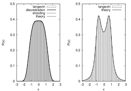
Figure 3: Stationary solutions to the Smoluchowski-Fokker-Planck and to the fractional Fokker-Planck equations associated with the diffusion ($\alpha=2$, left panel) and superdiffusion ($\alpha=1$, right panel) in a quartic potential $V(x)=x^{4}/4$. For $\alpha=2$ numerical results were constructed by discretization techniques and shooting methods dybiec2007c . Simulation parameters: $N=10^{6}$, $\Delta t=10^{-3}$, $N_{\mathrm{bins}}=100$ and $T_{\mathrm{max}}=10$.

III.1 Parabolic potential and algorithm testing

For $\sigma=1$, the fractional Fokker-Planck equation (II) can be rewritten in the Fourier space in the form of

$$\frac{\partial\hat{P}(k,t)}{\partial t}=\hat{\mathbf{V}}\hat{P}(k,t)-|k|^{\alpha}\hat{P}(k,t),$$ (9)

where $\hat{\mathbf{V}}$ is the operator giving the Fourier representation of the potential, which can be found in a closed form only in the simplest cases, e.g. for polynomial potentials. In the case of asymmetric distribution the analogous equation reads

$$\frac{\partial\hat{P}(k,t)}{\partial t}=\hat{\mathbf{V}}\hat{P}(k,t)-|k|^{\alpha}\left[1-i\beta\mbox{sign}(k)\tan\frac{\pi\alpha}{2}\right]\hat{P}(k,t).$$ (10)

The choice of the parabolic potential $V(x)=x^{2}/2$, see Fig. 1, results in its Fourier transform $\hat{\mathbf{V}}=-k\frac{\partial}{\partial k}$. For symmetric $\alpha$-stable noises, the corresponding equation for the stationary PDFs is chechkin2002 ; chechkin2003

$$\frac{\partial\hat{P}(k)}{\partial k}=-\mathrm{sign}k|k|^{\alpha-1}\hat{P}(k),$$ (11)

and its solution in the Fourier space reads

$$\hat{P}(k)=\exp\left(-\frac{|k|^{\alpha}}{\alpha}\right),$$ (12)

i.e., the stationary solution is a symmetric Lévy distribution, see Eqs. (2) and (3). Consequently, the variance of the stationary solution is infinite. Therefore, the parabolic potential is not sufficient to produce bounded states for a particle subject to the action of a Lévy noise jespersen1999 ; chechkin2002 ; chechkin2003 ; chechkin2004 ; dubkov2005b . For potentials steeper than the parabolic well, the confinement of superdiffusive trajectories becomes possible but, additionally, the additive Lévy white noise could induce bimodality in the stationary PDF.

For general $\alpha$-stable driving ($\alpha\neq 1$) the stationary solutions obey the equation

$$\frac{\partial\hat{P}(k)}{\partial k}=-\mathrm{sign}k|k|^{\alpha-1}\hat{P}(k)+i\beta\tan\frac{\pi\alpha}{2}|k|^{\alpha-1}\hat{P}(k),$$ (13)

and its solutions is

$$\hat{P}(k)=\exp\left[-\frac{|k|^{\alpha}}{\alpha}\left(1-i\beta\mbox{sign}(k)\tan\frac{\pi\alpha}{2}\right)\right].$$ (14)

For the nonzero asymmetry parameter, $\beta$, like for the symmetric noise, the stationary probability density function is a stable law with the same stability index $\alpha$ and the asymmetry parameter $\beta$ and a different scale parameter $\sigma^{\prime}=\sigma\alpha^{-1/\alpha}$ (here $\sigma^{\prime}=\alpha^{-1/\alpha}$). The location parameter $\mu$ of the resulting distribution is zero. The existence of these analytical results allows to use the case of parabolic potentials as a test bench for our simulation algorithms.

Thus, for the testing purposes, large samples of long realizations of the stochastic process given by Eq. (4) were constructed. Using these samples the values of the distributions parameters have been estimated applying special software stable . Estimated values of distributions parameters are in good agreement with theoretical values, see Tabs. 1–3. Techniques of estimation of the stable distribution parameters are based on the evaluation of quantiles and characteristic functions, and on maximum likelihood methods marinelli2000 or direct use of time series siegert2001 . Results obtained by quantile methods and characteristic function estimation seems to be more consistent with theoretical values than results following from maximum likelihood, see Tabs. 1–3. The largest differences between theoretical and estimated values of parameters are observed for the location parameter $\mu$. In some situations, marked with $*$, the program used stable warns about numerical problems in evaluation of the distributions parameters. To check whether results are influenced by the length of simulation results for $T_{\mathrm{max}}=10$ and $T_{\mathrm{max}}=15$ were compared. Estimated values of parameters for both values of $T_{\mathrm{max}}$ are consistent. Therefore, only results for $T_{\mathrm{max}}=15$ are presented, see Tabs. 1–3.

$\alpha$	$\beta$	$\sigma$	$\mu$
0.5	-1	4	0
0.502	-0.964	4.186	-5.43$\times 10^{-2}$
0.499	-1.000	3.978	-1.39$\times 10^{-2}$
0.500	-0.997	2.541	-6.81$\times 10^{-2}$
0.5	-0.5	4	0
0.500	-0.500	3.986	-1.76$\times 10^{-3}$
0.500	-0.498	3.992	-1.08$\times 10^{-2}$
0.514	-0.499	4.023	6.19$\times 10^{-2}$
0.5	0	4	0
0.500	0.001	3.993	-6.16$\times 10^{-3}$
0.501	0.000	3.998	6.24$\times 10^{-3}$
0.515	0.000	4.055	-1.68$\times 10^{-3}$
0.5	0.5	4	0
0.502	0.503	3.988	-3.00$\times 10^{-2}$
0.500	0.502	3.979	-1.35$\times 10^{-2}$
0.515	0.500	4.020	-6.52$\times 10^{-2}$
0.5	1	4	0
0.503	0.981	4.104	-2.04$\times 10^{-2}$
0.500	1.000	3.986	5.90$\times 10^{-4}$
0.462	0.990	7.844	-0.19

Table 1: Theoretical and estimated values of stationary PDF parameters. In every cell numbers in bold indicate theoretical values of parameters, followings rows estimated parameters using quantile evaluation (2^nd row), characteristic function evaluation (3^rd row) and maximum likelihood method (4^th row). Distributions’ parameters were estimated by use of stable . Simulations’ parameters: $T_{\mathrm{max}}=15$, $\Delta t=10^{-3}$. Samples contain not less than $10^{6}$ elements. $*$ indicates cases when the software applied warned about some problems in estimation of sample parameters.

$\alpha$	$\beta$	$\sigma$	$\mu$
1.1	-1	0.92	0
1.096	-1.000	1.237	-2.82
1.097	-1.000	0.917	-0.2
1.100	-1.000	0.917	2.70$\times 10^{-4}$
1.1	-0.5	0.92	0
1.099	-0.505	0.916	-4.15$\times 10^{-2}$
1.101	-0.501	0.917	1.58$\times 10^{-2}$
1.100	-0.501	0.917	-5.55$\times 10^{-3}$
1.1	0	0.92	0
1.098	-0.001	0.917	-7.83$\times 10^{-3}$
1.098	0.002	0.916	8.93$\times 10^{-3}$
1.099	-0.001	0.917	-5.05$\times 10^{-3}$
1.1	0.5	0.92	0
1.098	0.497	0.916	4.00$\times 10^{-2}$
1.099	0.496	0.917	1.84$\times 10^{-2}$
1.099	0.496	0.917	2.33$\times 10^{-2}$
1.1	1	0.92	0
1.101	1.000	1.237	2.41
1.100	1.000	0.918	-1.68$\times 10^{-2}$
1.100	1.000	0.918	4.17$\times 10^{-3}$

Table 2: Continuation of Table 1 ($\alpha=1.1$).

$\alpha$	$\beta$	$\sigma$	$\mu$
1.8	-1	0.72	0
1.798	-0.994	0.721	1.25$\times 10^{-3}$
1.800	-1.000	0.722	1.54$\times 10^{-3}$
1.829	-0.990	0.723	2.03$\times 10^{-2}$
1.8	-0.5	0.72	0
1.806	-0.531	0.723	-2.02$\times 10^{-3}$
1.799	-0.498	0.722	-4.49$\times 10^{-4}$
1.849	-0.545	0.729	1.17$\times 10^{-2}$
1.8	0	0.72	0
1.800	-0.002	0.722	-1.08$\times 10^{-3}$
1.798	-0.001	0.721	-5.69$\times 10^{-4}$
1.838	0.001	0.727	-2.69$\times 10^{-4}$
1.8	0.5	0.72	0
1.799	0.491	0.722	-2.50$\times 10^{-3}$
1.801	0.496	0.721	-2.43$\times 10^{-3}$
1.850	0.536	0.728	-1.46$\times 10^{-2}$
1.8	1	0.72	0
1.799	0.995	0.720	1.72$\times 10^{-3}$
1.798	0.988	0.720	6.72$\times 10^{-4}$
1.830	0.990	0.722	-1.74$\times 10^{-2}$

Table 3: Continuation of Table 1 ($\alpha=1.8$).

III.2 Quartic potential

For the quartic potential $V(x)=x^{4}/4$ ($\hat{\mathbf{V}}=k\frac{\partial^{3}}{\partial k^{3}}$) and symmetric $\alpha$-stable noises, fractional Fokker-Planck equation in the Fourier space has the form

$$\frac{\partial^{3}\hat{P}(k)}{\partial k^{3}}=\mathrm{sign}k|k|^{\alpha-1}\hat{P}(k).$$ (15)

The solution of Eq. (15) is known for $\alpha=1$ chechkin2002 ; chechkin2003 , $\hat{P}_{\alpha=1}(k)=\frac{2}{\sqrt{3}}\exp\left(-\frac{|k|}{2}\right)\cos\left(\frac{\sqrt{3}|k|}{2}-\frac{\pi}{6}\right),$ and the corresponding stationary solution in the real space reads

$$P_{\alpha=1}(x)=\frac{1}{\pi(1-x^{2}+x^{4})}.$$ (16)

The stationary solutions (16) of Eq. (15) have two main properties. First of all the stationary PDFs are not of the Boltzmann type, as typical for the stationary states for system driven by Lévy white stable noises with the stability index $\alpha<2$ eliazar2003 . Additionally, the stationary probability density function for a quartic Cauchy oscillator is bimodal, with extremes located at $x=\pm\nicefrac{{1}}{{\sqrt{2}}}$ chechkin2002 ; chechkin2003 ; chechkin2004 . Fig. 3 presents stationary PDFs obtained by the simulation of the Langevin equation (4) along with theoretical lines for the Gaussian (left panel) and Cauchy (right panel) quartic oscillators. Moreover, the parabolic addition to the quartic potential $V(x)=ax^{2}/2+x^{4}/4$ $(a>0)$, can diminish or even destroy the bimodality of the stationary PDF chechkin2002 ; chechkin2003 ; chechkin2004 . Finally, for the general $\alpha$-stable driving and the quartic potential the stationary density fulfills

$$\frac{\partial^{3}\hat{P}(k)}{\partial k^{3}}=\mathrm{sign}k|k|^{\alpha-1}\hat{P}(k)-i\beta\tan\frac{\pi\alpha}{2}|k|^{\alpha-1}\hat{P}(k).$$ (17)

Quartic potentials pose some additional difficulties to Monte-Carlo simulations making it necessary to slightly modify the standard techniques of integration of stochastic differential equations driven by $\alpha$-stable Lévy type noise janicki1994 . Due to heavy tails of stable distribution large random pulses are much more likely to occur than in the Gaussian distribution leading to very long jumps from time to time putting a particle to the position where the force acting on it is very large. In this case approximating the deterministic drift by $-\Delta tV^{\prime}(x)$ is too inaccurate whatever small time step is chosen. It can result in switch of the particle to the other side of the origin in such a way that new particle’s position is more distant from the origin than the initial one leading to numerical instability and escape of the particle to infinity dybiecphd . Of course, this effect is weaker when smaller integration step is used. However, taking smaller steps was proven not to give an effective solution to the problem. Our approach to it is based on separating noise and deterministic drift and integrating the last one analytically, by solving the differential equation $\dot{x}(t)=-V^{\prime}(x)$ to obtain $x(t+\Delta t)$ for a given initial condition $x(t)$. Such a step (involving the solution of an algebraic equation) is more time-consuming than the Euler integration step and is absolutely superfluous for small and moderate $x$. Therefore, exact integration of the deterministic part is performed only for large $x$, $|x|>x_{\mathrm{tr}}$, while the noisy part is always integrated in the standard Euler way. In the simulations we took $x_{\mathrm{tr}}=15$ as motivated by analytical estimates and by numerical tests. For testing purposes constructed numerical results for the Cauchy noise ($\alpha=1$) were compared with the known analytical solution, see right panel of Fig. 3, leading to the excellent level of agreement.

III.3 Double well potential

Figure 4: Influence of the time step of integration and duration of simulation on portion of non escaped trajectories at time $T_{\mathrm{max}}$ for $V(x)=x^{4}/4-x^{2}/2$. $x_{\mathrm{tr}}$ represents threshold value of $x$ such that for $|x|>x_{\mathrm{tr}}$ deterministic part of Eq. (4) is integrated analytically. The case $x_{\mathrm{tr}}=10^{12}$ corresponds simply to the standard Euler scheme. For more details see the text.

Figure 5: Stationary states for the generic double well potential model subjected to the $\alpha$-stable driving with $\alpha=0.5$ and various $\beta$. Simulation parameters: $N=10^{6}$, $\Delta t=10^{-3}$, $N_{\mathrm{bins}}=100$, $x_{\mathrm{tr}}=15$ and $T_{\mathrm{max}}=10$. Stationary states for totally skewed noise, i.e., $\beta=\pm 1$ are one-sided.

Figure 6: The same as in Fig. 5 for $\alpha=1.1$.

Figure 7: The same as in Fig. 5 for $\alpha=1.8$.

The results for the double-well potential model, see Fig. 1, were constructed by the numerical method described in the previous section (Section III.2). Furthermore, we compared the influence of decreasing time step of integration and $x_{\mathrm{tr}}$. The results of comparison of both methods of reduction of number of numerical escapes are summarized in Fig. 4 where the influence of the time step of integration $\Delta t$, duration of the simulation $T_{\mathrm{max}}$ on the portion of valid (non escaped) trajectories are compared.

Stationary solutions shown in Figs. 5–7 are obtained for the generic double well potential model, i.e., $V(x)=x^{4}/4-x^{2}/2$. In the simulation the whole allowed range of $\alpha$ and $\beta$ was examined, in figures only a limited choice of representative values of noise parameters is presented, namely the same as ones used in Tabs. 1–3. For $\alpha<1$ with $|\beta|=1$ stable distributions are one-sided, therefore, stationary solutions for $\alpha=0.5$ with $\beta=\pm 1$ are different from zero only on the one side of the origin. For $|\beta|<1$ stable distributions takes all real values as manifested by nonzero probability for all $x$, see Fig. 5. Furthermore, the symmetry of noise and the potential is reflected in the symmetry of stationary densities, i.e., solutions for $-\beta$ can be constructed by the reflection of the solutions for $\beta$, see Figs. 5–7. For $\beta=0$ with any $\alpha$ stationary densities are bimodal and symmetric along $x=0$. For $\alpha>1$, the support of stable densities as well as the stationary distributions is whole real line. Consequently, even extreme values of the asymmetry parameter $\beta=\pm 1$ are not sufficient to switch the probability mass to the one side of the origin, see Figs. 6–7. Furthermore, it is well documented in the lower panel of Fig. 8 where $P(\mathrm{left})=\int_{-\infty}^{0}P(x)dx$ is presented. Theoretical considerations as well as the probability of being in the left state, $P(\mathrm{left})$, indicate that stationary densities can be one-sided only for some totally skewed $\alpha$-stable noises with small $\alpha$, i.e., $\beta=\pm 1$ with $\alpha\ll 1$. For $\alpha>1$ with $\beta=\pm 1$ two maxima of stationary PDFs are visible. In upper panel of Fig. 8 locations of the median value, which may be considered as the next measure of asymmetry of stationary probability densities, are presented.

Very small values of $\alpha$ ($\alpha<0.5$) pose special difficulties for simulations. Our simulation of Eq. (4) starts with the initial condition $x(0)=0$. The initial transient peak of the probability density at this value is rather persistent for small $\alpha$, so that the simulation time has to be long. On the other hand in this case simulations are prone to escape of trajectories to “infinity” due to too strong noise pulses and require very small $\Delta t$, so that the overall quality of such results is not very good. Therefore, the results for $\alpha<0.5$ are not presented here.

Figure 8: Median (quantile $q_{0.5}$) of the stationary probability density $P(x)$ (upper panel) and asymmetry of stationary distributions measured as the fraction of the probability mass on the left hand side of the origin, i.e., $P(\mathrm{left})=\int_{-\infty}^{0}P(x)dx$ (lower panel). For symmetric noises resulting stationary densities are symmetric along $x=0$ and consequently $P(\mathrm{left})=1/2$ and $q_{0.5}=0$. Different symbols correspond to different values of the stability index $\alpha$: ‘$\circ$’ $\alpha=0.5$, ‘$\times$’ $\alpha=1.1$ and ‘$\square$’ $\alpha=1.8$.

Another method to present the results for stationary distributions is the use of the effective potential. In general, the same stationary probability densities that are recorded for the double well system driven by $\alpha$-stable noise, see Eq. (4), can be observed in the Gaussian regime in the effective potential $V_{\mathrm{eff}}(x)=-\ln P(x)$. Sample effective potentials corresponding to stationary states for $\alpha=1.1$ from Fig. 6 are depicted in Fig. 9. The same stationary solutions can be observed for motion in a simple potential, like double well potentials, and $\alpha$-stable stochastic driving or for potentials of the complicated form, see Fig. 9, and standard white Gaussian driving. Despite the fact that stationary states are the same, other characteristics of these two processes are different.

Figure 9: Effective potentials $V_{\mathrm{eff}}(x)=-\ln P(x)$ corresponding to stationary densities from Fig. 6. The effective potential $V_{\mathrm{eff}}(x)$ together with the white Gaussian noise results in stationary densities of the model (4) which are presented in Fig. 6.

IV Summary and conclusions

In the present work we investigated the form of stationary probability densities of a position of a particle subject to a deterministic potential force and to a Lévy noise, paying special attention to the case of asymmetric stable noises. Stationary density functions for system driven by $\alpha$-stable Lévy noises ($\alpha\neq 2$), if they exist, are not of the Boltzmann-Gibbs form.

For parabolic potential the stationary density functions are $\alpha$-stable laws with the same stability index $\alpha$ and asymmetry parameter $\beta$ as ones of the noise. The only difference is the scale parameter of the resulting distribution. Therefore, this case can serve as a benchmark for our simulation algorithms. By use of the special software stable for estimation of stable law parameters, the parameters of stationary densities have been evaluated leading to a very good level of agreement between theoretical and estimated values of parameters. Natural consequence of the Lévy type of the stationary densities for parabolic potential is divergence of the variance of the particle position. To produce bounded states, i.e., states with finite variance of a position, potentials steeper than quadratic are necessary. Thus, for the quartic potential variance of stationary densities is finite. Furthermore, for white Cauchy noise analytical solutions to the stationary problem is known. Here again, numerical results fully agree with earlier chechkin2002 ; chechkin2003 theoretical findings.

In the case of Gaussian noise ($\alpha=2$) the symmetry of stationary density (being the Boltzmann-Gibbs equilibrium distribution) reflects symmetries of the underlying potential: the asymmetric densities correspond to asymmetric potentials, i.e., to deterministic forces which break the symmetry of the initial problem. The Gaussian noise itself is always symmetric. For systems driven by Lévy noises ($\alpha\neq 2$), an asymmetric stable noise together with symmetric static potential is sufficient to produce asymmetric stationary densities. In this situation the asymmetry of stationary states originates from the asymmetry of the stochastic driving and can be controlled by changing the parameters of the noise.

Our main studies have been performed for the generic symmetric double well potential model. Here the asymmetry of the stationary distribution (as measured by the probability of being in the left/right state or location of the median) was investigated as a function of the parameters of the noise. The asymmetry of stationary state decreases with increasing $\alpha$, see Fig. 8. Finally for $\alpha=2$ with any value of the asymmetry parameter $\beta$ Gaussian scenario is recovered and stationary density is fully symmetric. We also checked whether stable asymmetric noise can produce unimodal stationary PDFs in the double well potential. Such situation can indeed be observed for fully asymmetric noises ($|\beta|=1$) with $\alpha\ll 1$, e.g. for the Lévy-Smirnoff noise ($\alpha=0.5$, $\beta=1$).

Appendix A Dimensionality of the Langevin equation

We have investigated the dynamic stochastic process modeled by the (overdamped) Langevin equation of the form

$$\dot{x}(t)=\frac{f(x)}{\gamma m}+D^{1/\alpha}\zeta(t)=\frac{f(x)}{\gamma m}+\sigma\zeta(t),$$ (18)

where: $x$ – is a position of the particle, $\gamma$ – stands for a friction coefficient, $m$ – is particle’s mass, $D$ ($\sigma$) – represents strength of the noise and $\zeta(t)$ – is Lévy stable white noise characterized by the stability index $\alpha$ ($\alpha\in(0,2]$) and the asymmetry parameter $\beta$ ($\beta\in[-1,1]$). The force acting on a particle is determined by the external potential, $f(x)=-dV(x)/dx$.

Corresponding units in Eq. (18) are: $[x]=[\mbox{length}]$, $[\gamma]=1/[t]$, $[f(x)]=[V^{\prime}(x)]=[m]\times[\mbox{length}]/[t]^{2}=[\mbox{force}]$, $[V(x)]=[\mbox{force}]\times[\mbox{length}]=[\mbox{energy}]$, $[D]=[\mbox{length}]^{\alpha}/[t]$ ($[\sigma]=[\mbox{length}]/[t]^{1/\alpha}$) and $[\zeta(t)]=1/[t]^{1-1/\alpha}$. Stability index $\alpha$ and asymmetry parameter $\beta$ are dimensionless. In the asymptotic limit of $\alpha=2$ the Lévy white noise is equivalent to the Gaussian white noise and it has standards units, i.e. $[\zeta_{\alpha=2}(t)]=[\xi(t)]=1/\sqrt{[t]}$.

By the set of transformation: $t\to t/t_{0}$ and $x\to x/x_{0}$. Eq. (18) can be transformed to the dimensionless form

$$\dot{x}(t)=f(x)+D^{1/\alpha}\zeta(t)=f(x)+\sigma\zeta(t),$$ (19)

which is of the same type like Eq. (1) because the (rescaled) noise intensity can be incorporated to the distribution of the particle’s position increments. An alternative way of getting dimensionless form of Eq. (18) can be found in a recent work chechkin2007 .

For the single-well potential $V(x)=ax^{n}/n$

$$t_{0}=\frac{x_{0}^{\alpha}}{D},\;\;\;\;\;x_{0}=\left[\frac{D\gamma m}{a}\right]^{\frac{1}{n-2+\alpha}}.$$ (20)

Thus $V(x)\to x^{n}/n$ and $\sigma\to 1$. Therefore, for the single minima potential, the only relevant parameters are $\alpha$ (stability index) and $\beta$ (asymmetry parameter).

For the generic double-well potential $V(x)=-ax^{2}/2+bx^{4}/4$

$$t_{0}=\frac{\gamma m}{a},\;\;\;\;\;x_{0}^{2}=\frac{\gamma m}{bt_{0}}=\frac{a}{b}.$$ (21)

Thus $V(x)\to-x^{2}/2+x^{4}/4$ and $\sigma\to\sigma t_{0}^{1/\alpha}/x_{0}$. In consequence, for the double-well potential, the only relevant parameters in a dimensionless form of Eq. (18) are the Lévy noise parameters $\alpha$ and $\beta$, and a (rescaled) noise strength. From the above analysis, it is clear that the choice of $x_{0}$, $t_{0}$ introduce scales to the system which are directly related to its dynamical parameters.

- (1) Lévy Flights and Related Topics in Physics, edited by M. F. Schlesinger, G. M. Zaslavsky, U. Frisch (Springer Verlag, Berlin, 1995).
- (2) Lévy Processes: Theory and Applications, edited by O. E. Barndorff-Nielsen, T. Mikosch, S. I. Resnick (Birkhäuser, Boston, 2001).
- (3) S. Jespersen, R. Metzler and H. C. Fogedby, Phys. Rev. E 59, 2736 (1999).
- (4) P. D. Ditlevsen, Phys. Rev. E 60, 172 (1999).
- (5) B. Kosko and S. Mitaim, Phys. Rev. E 64, 051110 (2001).
- (6) B. Dybiec and E. Gudowska-Nowak, Phys. Rev. E 69, 016105 (2004).
- (7) B. Dybiec and E. Gudowska-Nowak, Fluct. and Noise Lett. 4, L273 (2004).
- (8) B. Dybiec and E. Gudowska-Nowak, Proc SPIE 5467, 411 (2004).
- (9) B. Dybiec, E. Gudowska-Nowak and P. Hänggi, Phys. Rev. E 73, 046104 (2006).
- (10) B. Dybiec and E. Gudowska-Nowak, Acta Physica Polonica B 37, 1479 (2006).
- (11) B. Dybiec, E. Gudowska-Nowak and P. Hänggi, Phys. Rev. E 75, 021109 (2007).
- (12) A. V. Chechkin, J. Klafter, V. Yu. Gonchar, R. Metzler and L. V. Tanatarov, Chem. Phys. 284, 233 (2002).
- (13) A. V. Chechkin, J. Klafter, V. Yu. Gonchar, R. Metzler and L. V. Tanatarov, Phys. Rev. E 67, 010102 (2003).
- (14) A. V. Chechkin, V. Yu. Gonchar, J. Klafter, R. Metzler and L. V. Tanatarov, J. Stat. Phys. 115, 1505 (2004).
- (15) I. M. Sokolov, V. V. Belik, Physica A 330, 46 (2003).
- (16) B. Dybiec, Stochastic Resonant Effects in Systems Driven by Stable Noises, PhD Thesis, Faculty of Physics, Astronomy and Applied Computer Sciences, Marian Smoluchowski Institute of Physics, Jagellonian University, Kraków, Poland, 2005.
- (17) W. Feller, An introduction to Probability Theory and its Applications (John Wiley, New York, 1968).
- (18) A. Janicki and A. Weron, Simulation and Chaotic Behavior of -Stable Stochastic Processes (Marcel Dekker, New York, 1994).
- (19) A. Janicki, Numerical and Statistical Approximation of Stochastic Differential Equations with Non-Gaussian Measures (Hugo Steinhaus Centre for Stochastic Methods, Wrocław, 1996).
- (20) I. Eliazar and J. Klafter, J. Stat. Phys. 111, 739 (2003).
- (21) I. Eliazar, J. Klafter, Physica A 336, 219 (2004).
- (22) I. Podlubny, Fractional Differential Equations (Academic Press, San Diego, 1998).
- (23) G. H. Weiss and A. Szabo, Physica A 119, 569 (1983).
- (24) M. O. Cáceras, J. Phys. A 32, 6009 (1999).
- (25) A. Janicki, A. Weron, Stat. Sci. 9, 109 (1994).
- (26) A. Janicki, A. Izydorczyk, Computer methods in stochastic modelling (in Polish) (Wydawnictwa Naukowo Techniczne, Warszawa, 2001).
- (27) J. P. Nolan, Stable Distributions - Models for Heavy Tailed Data (Birkhäuser, Boston, 2007).
- (28) A. Weron and R. Weron, Lecture Notes in Physics 457, 379 (1995).
- (29) R. Weron, Statist. Probab. Lett. 28, 165 (1996).
- (30) V. V. Yanovsky, A. V. Chechkin, D. Schertzer, A. V. Tur, Physica A 282, 13 (2000).
- (31) D. Schertzer and M. Larchevêque, J. Duan, V. V. Yanowsky, S. Lovejoy, J. Math. Phys. 42, 200 (2001).
- (32) M. Di Paola and M. Vasta, ASME Applied Mechanics Division 254, 207 (2003).
- (33) D. Brockmann, I. M. Sokolov, Chem. Phys. 284, 409 (2002).
- (34) R. Metzler, E. Barkai and J. Klafter, Europhys. Lett. 46, 431 (1999).
- (35) R. Metzler and J. Klafter, J. Phys. A: Math. Gen. 37, R161 (2004).
- (36) A. A. Dubkov and B. Spagnolo, Fluc. Noise Lett. 5, L267 (2005).
- (37) E. Barkai, Phys. Rev. E 68, 055104 (2003).
- (38) E. Barkai, J. Stat. Phys. 115, 1572 (2004).
- (39) W. H. Press, S. A. Teukolsky, W. T. Vetterling and B. P. Flannery, Numerical Recipes. The art of scientific computing (Cambridge University Press, Cambridge, 1992).
- (40) E. Abdel-Rehim, Modelling and Simulating of Classical and Non-Classical Diffusion Processes by Random Walks, PhD Thesis, Department of Mathematics and Informatics, Freie Universität, Berlin, Germany, 2004.
- (41) B. Dybiec, L. Schimansky-Geier, Eur. Phys. J. B 57 313, (2007).
- (42) R. Gorenflo, F. Mainardi, D. Moretti, G. Pagnini, P. Paradisi, Chem. Phys. 284, 521 (2002).
- (43) M. M. Meerschaert, Ch. Tadjeran, J. Comp. App. Math. 172, 65 (2004).
- (44) J. P. Nolan, STABLE, http://academic2.american.edu/~jpnolan/.
- (45) C. Marinelli and S. T. Rachev, in Applied Mathematics Reviews, edited by G. A. Anastassiou (World Scientific Publishing, River Edge, NJ, 2000), Vol. 1, p. 285.
- (46) S. Siegert and R. Friedrich, Phys. Rev. E 64, 041107 (2001).
- (47) A. V. Chechkin, O. Yu. Sliusarenko, R. Metzler and J. Klafter, Phys. Rev. E 75, 041101 (2007).