Adaptive mesh computation of polycrystalline pattern formation using a renormalization-group reduction of the phase-field crystal model

Abstract

We implement an adaptive mesh algorithm for calculating the space and time dependence of the atomic density field during materials processing. Our numerical approach uses the systematic renormalization-group formulation of the phase field crystal model to provide the underlying equations for the complex amplitude of the atomic density field—a quantity that is spatially uniform except near topological defects, grain boundaries and other lattice imperfections. Our algorithm is a hybrid formulation of the amplitude equations, combining Cartesian and polar decompositions of the complex amplitude. We show that this approach leads to an acceleration by three orders of magnitude in model calculations of polycrystalline domain formation in two dimensions.

I Introduction

A fundamental theoretical and computational challenge in materials modeling is that of concurrently treating phenomena over a wide range of length and time scales. For example, in studying the mechanical response of polycrystalline materials, one must take into account the dynamics and interactions of vacancies, impurities, dislocations and grain boundaries, on time scales ranging from atomic vibrations to system-wide diffusion times.

Numerous approaches to handling the wide range of length scales have been proposed Phillips (2001), including quasi-continuum methods Tadmor et al. (1996); Shenoy et al. (1998); Knap and Ortiz (2001); Miller and Tadmor (2002), the heterogeneous multiscale method E et al. (2003); E and Huang (2001), multi-scale molecular dynamics Rudd and Broughton (1998); Broughton et al. (1998); Denniston and Robbins (2004); Curtarolo and Ceder (2002), multigrid variants Fish and Chen (2004) and phase field models Langer (1986); Karma and Rappel (1998); Beckermann et al. (1999); Warren et al. (2003). In general one can classify different techniques as being either atomistic or continuum, and differentiate them further by the characteristic time scale: density functional theory (DFT), for a quantum mechanical description of processes at the atomic time scale; molecular dynamics (MD) or Monte Carlo (MC) methods, appropriate for collective dynamics; and coarse-grained descriptions involving continuum fields at the mesoscale on diffusive time scales. The difficulty of merging descriptions at different length and time scales limits the effective application of most of these methods. Lack of a continuous transition between scales can induce artifacts, such as spurious reflections in a transition region between two levels Vvedensky (2004); E and Huang (2001). Further, any method using molecular dynamics is typically restricted to sub-nanosecond time scales, whereas many interesting phenomena during materials processing, such as microstructural pattern formation, recrystallization, heat and solute diffusion, dislocation glide, etc., occur over time scales which are typically greater than $10^{-6}$s.

One continuum approach that has been used successfully, especially in the multiscale modeling of solidification problems Provatas et al. (2005), is the phase-field method Langer (1986). Through the effective use of asymptotics Karma and Rappel (1998) and adaptive mesh refinement Provatas et al. (1998a); Jeong et al. (2001), the phase-field method has been used to span several orders of magnitude in length, from microns to centimeters. Extensions of the method by Kobayashi and co-workers Kobayashi et al. (1998, 2000), and Warren Warren et al. (2003) also make it possible to model polycrystalline systems. Special forms of the free energy that incorporate strain energy have been used to model the qualitative features of strain-induced phase transformations Onuki (1989a, b); Muller and Grant (1999); Kassner et al. (2001); Karma et al. (2001); Haataja et al. (2005). The phase-field method represents a coarse-graining in space to length scales much greater than those of the interfaces and defects of interest in this work. As a result, the kinetic coefficients that emerge in the final continuum equations are phenomenological, and can be related to experimentally-measurable parameters only after a suitable asymptotic matching of the phase field equations with corresponding sharp-interface models Karma (2001); Echebarria et al. (2004); Provatas et al. (2005). As such, traditional phase field models do not fundamentally embody the emergent kinetic and elasto-plastic mechanisms that originate at the atomic scale. Perhaps the most important limitation of phase field models is that, in general, they do not preserve any record of the underlying crystal lattice, so that ad hoc approaches must be used to model the variety of phenomena which result from lattice interactions.

The phase field crystal (PFC) model Elder et al. (2002); Elder and Grant (2004) is a promising extension of the phase field model approach, in which the equilibrium configuration of an atomic density field is constructed to be periodic, rather than uniform in space. The conserved dynamics of the PFC model then naturally reproduce many of the non-equilibrium processing dynamics arising in real polycrystalline materials. The PFC model is founded on the insight that a free energy functional that is minimized by a periodic field natively includes elastic energy, anisotropy and symmetry properties of that field. Thus the model naturally incorporates all properties of a crystal that are determined by symmetry, as well as vacancies, dislocations, and other defects. Moreover, the PFC model represents the evolution of the system over a time scale that is much longer than the vibrational period of atoms (${\cal{O}}(10^{-15}\mbox{s})$), but much shorter than the time scale of diffusive processes in the system, such as the viscous glide of dislocations, which typically occur over a time scale of ${\cal{O}}(10^{-6}\mbox{s})$. The PFC model yields a relatively simple and well-behaved partial differential equation (PDE) for the evolution of the time-averaged density, giving it access to phenomena occurring on atomic length scales, but over diffusive time scales. The PFC method is thus able to capture atomic-scale elasticity and the interaction of topological defects on the same time scales that govern diffusive processes during phase transformations in pure materials Elder and Grant (2004); Berry et al. (2006); Stefanovic et al. (2006) and alloys Elder et al. (2006).

As with any model that resolves at the atomic scale, the PFC model is limited in its ability to model systems of realistic dimensions, because the computational grid must resolve the periodicity of the field. For grid converged results, a minimum of 9 grid points per period are required. In a physical system, the periodicity represents interatomic distance, ${\cal{O}}(10^{-10}{\rm m})$. Thus, to simulate a system having a characteristic dimension of one micron would require about $10^{5}$ degrees of freedom per spatial dimension on a uniform computational mesh. This would be a heroic computation in 2-D, and well beyond reach in 3D, even with the use of massive parallelization. Furthermore, the periodic lattice precludes the effective use of adaptive mesh refinement (AMR) algorithms.

The first three authors have recently described an approach to overcome this difficulty Goldenfeld et al. (2005, 2006), using the perturbative renormalization group (RG) method Chen et al. (1996); Nozaki and Oono (2001) to systematically coarse-grain the PFC equationAthreya et al. (2006). The basic idea is to obtain renormalization group equations of motion for the complex amplitude of the periodic density field, a quantity whose modulus and phase are spatially uniform except near regions of lattice disruption, such as at grain boundaries and at topological defects. From the complex amplitude, it is possible to reconstruct the atomic-scale density field at least within the one-mode approximation, and to compute non-trivial materials properties and dynamics to high accuracy (within one percent)Goldenfeld et al. (2005, 2006). This approach, which we will sometimes denote as the PFC-RG method, is much faster than solving the PFC equation directly, because the complex amplitude varies on much larger spatial length scales than the density itself, thus permitting the use of an adaptively-generated coarse mesh over much of the computational domainGoldenfeld et al. (2005). It is important to appreciate that the equations of motion for the complex amplitude must be rotationally-covariant, in order that a polycrystalline material or heterogeneous microstructure can be represented without any preferred orientations imposed; this is readily achieved using renormalization group methodsAthreya et al. (2006). However, in a practical computation, the reciprocal lattice vectors of the equilibrium crystal structure are represented within a particular basis, and there is the potential for interference between the density Fourier components and the basisGoldenfeld et al. (2005), giving rise to artifactual “fringes” or “beats” in the corresponding Fourier components. The overall density does not, of course, exhibit these interference fringes, but their presence in the individual components means that to be properly resolved, an adaptive mesh algorithm must generate grid refinement in their vicinity. As a result, efficient computation becomes compromised.

The purpose of this paper is to develop a computationally-efficient formulation of the PFC-RG method that enables the implementation of an AMR algorithm up to micro- and meso- length scales, without being deflected by artifacts arising from the choice of basis set. The approach is to use a hybrid representation of the complex amplitude, switching between Cartesian and polar coordinates as appropriate in a seamless fashion to avoid beating and coordinate singularities. The resultant description is fast, accurate and provides mesh refinement and coarsening in the physically correct locations, without artifacts arising from choice of basis or other implementation-dependent details. As such, our work represents a first step towards providing a systematic description of materials processing using continuum fields across all relevant length scales.

The remainder of this paper is organized as follows: We introduce the complex amplitude equations (interchangeably called the RG equations) in Section II and illustrate the interference or beat problem in the Cartesian representation of these equations that limits the effectiveness of AMR techniques. In Section III we introduce a polar formulation of the equations that addresses the problem of beats, but also exhibits coordinate singularities that make these equations unwieldy for numerical solution. We then present a new hybrid formulation in Section IV, which is a procedure for solving the Cartesian equations of Section II concurrently with a reduced form of the polar equations of Section III in different parts of the computational domain. In Section V the hybrid formulation of the RG equations is demonstrated to be amenable to solution using a new finite-difference-based AMR algorithm specifically developed for our RG equations. Section VI presents numerical simulations and results, including efficiency benchmarks that clearly demonstrate the computational advantage of our AMR-RG approach. Section VII concludes and presents directions for future work.

II The complex amplitude equations

II.1 Governing equations

In the PFC model, the evolution of the density $\rho$ is given by

$$\frac{\partial\rho}{\partial t}=\Gamma\nabla^{2}\left({\delta{\cal F}\over\delta\rho}\right)+\eta$$ (1)

where ${\cal F}$ is the free energy functional, which can be written as ${\cal F}=\int d\vec{r}\left(f\left(\rho,\nabla^{2}\rho,\ldots\right)\right)$, where $f$ is the local free energy density, $\Gamma$ is a constant and $\eta$ is a stochastic noise with zero mean and correlations $\langle\eta(\vec{r},t)\eta(\vec{r}^{\prime},t^{\prime})\rangle=-\Gamma k_{B}T\nabla^{2}\delta(\vec{r}-\vec{r}^{\prime})\delta(t-t^{\prime})$. The specific form of ${\cal F}$ is chosen such that at high temperatures ${\cal F}$ is minimized by a spatially uniform liquid state, and at low temperatures by a spatially periodic “crystalline” phase. Furthermore, $f$ must be chosen such that ${\cal F}$ is independent of crystal orientation. These constraints naturally incorporate both elastic and plastic deformations.

A free energy form that satisfies these criteria naturally produces mobile regions of liquid/solid coexistence separated by free surfaces, i.e., phase transformations. Elastic energy and defects in the crystalline phase arise from the requirement that ${\cal F}$ be minimized by a spatially periodic density field that is independent of crystal orientation. Elder et al. Elder et al. (2002); Elder and Grant (2004) demonstrated these properties of the model for a variety of applications, including studies of grain boundary energy, liquid phase epitaxial growth and the yield strength of nanocrystalline materials. The particular model they used made the following choice for the function $f$:

$$f=\rho\left(\alpha\Delta T+\lambda\left(q_{o}^{2}+\nabla^{2}\right)^{2}\right)\rho/2+u\rho^{4}/4$$ (2)

where $\alpha$, $\lambda$, $q_{o}$ and $u$ are model parameters that can be specified to match some specific material properties, such as Young’s modulus and lattice spacing Elder et al. (2002); Elder and Grant (2004). In order to discuss the dynamical behavior of the PFC model, it is useful to rewrite the free energy in dimensionless units: $\vec{x}\equiv\vec{r}q_{o}$, $\psi\equiv\rho\sqrt{u/\lambda q_{o}^{4}}$, $r\equiv a\Delta T/\lambda q_{o}^{4}$, $\tau\equiv\Gamma\lambda q_{o}^{6}t$ and $F\equiv{\cal F}u/\lambda^{2}q_{o}^{8-d}$ so that

$$F=\int d\vec{x}\left[\psi\left(r+(1+\nabla^{2})^{2}\right)\psi/2+\psi^{4}/4\right]$$ (3)

In these units the conservation law of Eq. (2) becomes

$$\frac{\partial\psi}{\partial t}=\nabla^{2}\left[\left(r+(1+\nabla^{2})^{2}\right)\psi+\psi^{3}\right]+\zeta$$ (4)

where $\langle\zeta(\vec{r}_{1},t_{1})\zeta(\vec{r}_{2},\tau_{2})\rangle={\cal E}\nabla^{2}\delta(\vec{r}_{1}-\vec{r}_{2})\delta(\tau_{1}-\tau_{2})$ and ${\cal E}\equiv uk_{B}Tq_{o}^{d-4}/\lambda^{2}$. Eq. (4), introduced by Elder et al Elder et al. (2002); Elder and Grant (2004), will be referred to as the PFC equation in what follows. This equation can be used in any dimension by simply introducing the appropriate form for the Laplacian operators.

The spatial density $\psi$ can be approximated in terms of the complex amplitude $A_{j}$ as

$$\psi\approx\sum_{j=1}^{3}A_{j}e^{i\mathbf{k}_{j}\cdot\mathbf{x}}+\sum_{j=1}^{3}A_{j}^{*}e^{-i\mathbf{k}_{j}\cdot\mathbf{x}}+\bar{\psi},$$ (5)

where

$$\mathbf{k}_{1} = k_{0}({-\vec{\mbox{i}}\sqrt{3}/2}-{\vec{\mbox{j}}/2})$$

$$\mathbf{k}_{2} = k_{0}{{\vec{\mbox{j}}}}$$

$$\mathbf{k}_{3} = k_{0}({\vec{\mbox{i}}\sqrt{3}/2}-{\vec{\mbox{j}}/2})$$ (6)

are the reciprocal lattice vectors of a crystal with hexagonal symmetry, and $k_{0}$ is the dominant wavenumber of the pattern. For all the calculations shown in this paper length has been scaled such that $k_{0}=1$, which corresponds to an interatomic spacing of $a_{0}=2\pi/(\sqrt{3}/2)$. The complex amplitude equations, which constitute a coarse-grained approximation to the PFC equation were shown in our earlier work Goldenfeld et al. (2005, 2006) to be given by

$$\frac{\partial A_{j}}{\partial t}=\widetilde{\mathcal{L}}_{j}A_{j}-3A_{j}|A_{j}|^{2}-6A_{j}\sum_{k:k\neq j}|A_{k}|^{2}-6\bar{\psi}\prod_{k:k\neq j}A_{k}^{*}$$ (7)

where $j,k\in[1,3]$ and

$$\widetilde{\mathcal{L}}_{j}=\left[1-\nabla^{2}-2i{\mathbf{k}_{j}}\cdot\nabla\right]\left[-r-3\bar{\psi}^{2}-\left\{\nabla^{2}+2i{\mathbf{k}_{j}}\cdot\nabla\right\}^{2}\right]$$ (8)

is a rotationally covariant operator. The superscript “$*$” denotes complex conjugation. The parameters $r\;(\leq 0)$ and $\bar{\psi}\;(\geq 0)$ control the bifurcation from a uniform liquid phase to a crystalline phase with hexagonal symmetry. Specifically, $r$ is proportional to the temperature quench from a critical temperature $T_{c}$, while $\bar{\psi}$ is the mean density in the system. We refer to this form as the Cartesian representation because the amplitudes are expressed along each coordinate direction.

The rotational covariance of the operator $\widetilde{\cal{L}}$ permits the incorporation of multiple crystal orientations using only the basis vectors in Eq. (II.1). To see this consider a density field $\psi$ defined by Eq. (5) with triangular lattice basis vectors $\mathbf{k}_{j}(\theta)$ (where $|\mathbf{k}_{j}(\theta)|=1$) that are rotated by an angle $\theta$ from the basis vectors $\mathbf{k}_{j}$ in Eq. (II.1), i.e.

$$\psi(\theta)=\sum_{j=1}^{3}A_{j}e^{i\mathbf{k}_{j}(\theta)\cdot\mathbf{x}}+\sum_{j=1}^{3}A_{j}^{*}e^{-i\mathbf{k}_{j}(\theta)\cdot\mathbf{x}}+\bar{\psi}.$$ (9)

Equation (9) describes the density field of a grain misoriented with respect to the basis vectors. Writing the basis vectors as $\mathbf{k}_{j}(\theta)=\mathbf{k}_{j}+\delta\mathbf{k}_{j}(\theta)$, where the vector $\delta\mathbf{k}_{j}(\theta)$ measures the rotation of each lattice vector, we obtain

$$\psi(\theta)=\sum_{j=1}^{3}A_{j}e^{i\delta\mathbf{k}_{j}(\theta)\cdot\mathbf{x}}e^{i\mathbf{k}_{j}\cdot\mathbf{x}}+\sum_{j=1}^{3}A_{j}^{*}e^{-i\delta\mathbf{k}_{j}(\theta)\cdot\mathbf{x}}e^{-i\mathbf{k}_{j}\cdot\mathbf{x}}+\bar{\psi},$$ (10)

or

$$\psi(\theta)=\sum_{j=1}^{3}A_{j}^{\theta}e^{i\mathbf{k}_{j}\cdot\mathbf{x}}+\sum_{j=1}^{3}{A_{j}^{\theta}}^{*}e^{-i\mathbf{k}_{j}\cdot\mathbf{x}}+\bar{\psi},$$ (11)

where

$$A_{j}^{\theta}=A_{j}e^{i\delta\mathbf{k}_{j}(\theta)\cdot\mathbf{x}}.$$ (12)

Thus grains arbitrarily misoriented from the global basis $\mathbf{k}_{j}$ can still be described in terms of $\mathbf{k}_{j}$ by suitably representing the complex amplitude $A_{j}$ in polar form according to Eq. (12). A straightforward way to include differently oriented grains in the system is to specify an initial condition via Eq. (11). By making the amplitude a non-uniform complex function with a periodic structure, multiple grain orientations are automatically included. Fig. 1 illustrates this idea. Fig. 1(a) shows the real component of one of the three complex amplitude functions $A_{j}$, specified by Eq. (12), and Fig. 1(b) shows the corresponding density field constructed using Eq. (11). Since Eq. (7) is rotationally covariant, it allows these “beat” structures in the amplitudes (and therefore the corresponding orientation of the grain) to be preserved as the system evolves, thereby enabling the representation of polycrystalline systems with a single set of basis vectors.

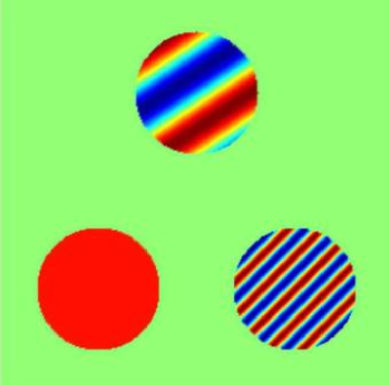
(a) $\Re(A_{1})$

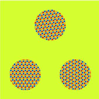
(b) $\psi$

Figure 1: (a) Real component of the complex amplitude $A_{1}$. As the grain in the bottom-left corner is aligned with the basis $\mathbf{k}_{j}$ in Eq. (II.1) its amplitude is constant, while amplitudes of the remaining misoriented grains have “beats”. (b) Density field $\psi$ reconstructed using Eq. (11). Clockwise from the lower left corner, $\theta=0$, $\pi/24$ and $\pi/6$.

II.2 Limitations of the Cartesian representation of Equation (7)

A straightforward approach to solving Eq. (7) is to determine the real and imaginary parts of the complex amplitudes $A_{j}$ directly, using the Cartesian definition. This leads to six equations that can be evolved concurrently using a suitable time integration scheme. The second order finite difference spatial discretizations of the Laplacian and gradient operators are given in the Appendix. This approach leads to limited success of AMR techniques because of the beats.

To illustrate this effect, we simulated heterogeneous nucleation and growth of a two-dimensional film, randomly placing twelve randomly oriented crystals of initial radius $8\pi$ in a square domain of side $256\pi$ with periodic boundary conditions. The largest misorientation angle between grains was $\theta=\pi/12$. The amplitude equations in Cartesian form were solved using an adaptively evolving mesh (described in detail below). The model parameters were $r=-0.25$ and $\bar{\psi}=0.285$, the smallest mesh spacing was $\Delta x_{min}=\pi/2$, while the largest mesh spacing at any given time was $\Delta x_{max}=2^{4}(\Delta x_{min})$ corresponding to 5 levels of refinement. On a uniform grid, this simulation requires $1025\times 1025=1,050,625$ nodes with the PFC equation, and $513\times 513=263,169$ nodes with the amplitude equations. A time step of $\Delta t=0.04$ was used.

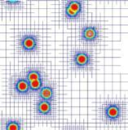
(a) t=0

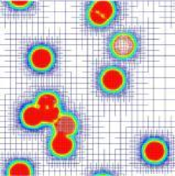
(b) t=88

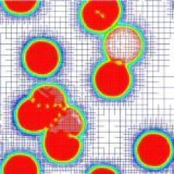
(c) t=168

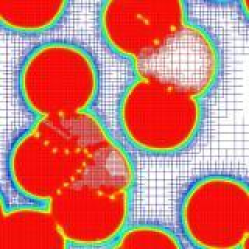
(d) t=248

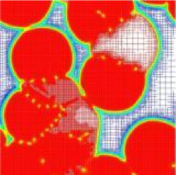
(e) t=320

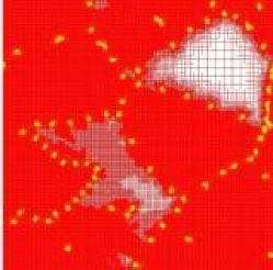
(f) t=552

Figure 2: (Color online) Evolution of a polycrystalline film simulated with complex amplitude equations, Eq. (7), on an adaptive grid. Note that the grid does not coarsen inside many of the grains (misoriented with respect to $\mathbf{k}_{j}$) because of the fine scale structure of the “beats”. The colored field plotted is the average amplitude modulus, which is “red” inside the crystal phase, “blue” in the liquid phase, “green” at the crystal/liquid interface, and “yellow” near defects.

Fig. 2 shows the crystal boundaries and grid structure at various times during the simulation. The field plotted is the average amplitude modulus, $\sum_{j=1}^{3}A_{j}/3$. Although the grid starts out quite coarse ($t=0$ and $t=88$) at several locations in the computational domain because of the large liquid fraction, this advantage falls off dramatically once the crystals evolve, collide, and start to form grain boundaries. In particular, once all the liquid freezes, only a few grains that are favorably oriented with respect to $\mathbf{k}_{j}$ show any kind of grid coarsening at all. Those that are greatly misorientated with respect to $\mathbf{k}_{j}$ lead to frequency beating, causing the number of nodes in the adaptive grid to increase rather than decrease. The polycrystal mesh shown in Fig. 2(f) has $219,393$ nodes, which is very near that on a uniform grid. Therefore the adaptive refinement algorithm applied to a Cartesian formulation of Eq. 7 gives at best a marginal improvement over a fixed grid implementation. The main purpose of this paper is to present a methodology for overcoming this problem.

III Complex amplitude equations in a polar representation

III.1 Governing equations

We find that the computational benefits of AMR are potentially greater if, instead of solving for the real and imaginary components of $A_{j}$, we solve for the amplitude moduli $\Psi_{j}=|A_{j}|$, and the phase angles $\Phi_{j}=\arctan(\Im(A_{j})/\Re(A_{j}))$, which are spatially uniform fields irrespective of crystal orientation. Together these two fields constitute a polar representation of $A_{j}$.

In this section we derive evolution equations for $\Psi_{j}$ and $\Phi_{j}$ directly from Eq. (7), by applying Euler’s formula for a complex number, i.e. $A_{j}=\Psi_{j}e^{i\Phi_{j}}$, and then by equating corresponding real and imaginary parts on the left- and right-hand sides of the resulting equations. In this manner we get the coupled system of equations,

$$\frac{\partial\Psi_{j}}{\partial t} = (r+3\bar{\psi}^{2})\left[-\Psi_{j}+\mathcal{C}^{\Re}(\Psi_{j},\Phi_{j})\right]-\left[\mathcal{C}^{\Re\Re}(\Psi_{j},\Phi_{j})-\mathcal{C}^{\Im\Im}(\Psi_{j},\Phi_{j})\right]$$ (13)

$$+\left[\mathcal{C}^{\Re\Re\Re}(\Psi_{j},\Phi_{j})-\mathcal{C}^{\Re\Im\Im}(\Psi_{j},\Phi_{j})-\mathcal{C}^{\Im\Im\Re}(\Psi_{j},\Phi_{j})-\mathcal{C}^{\Im\Re\Im}(\Psi_{j},\Phi_{j})\right]$$

$$-3\Psi_{j}\left(\Psi_{j}^{2}+2\sum_{k\neq j}\Psi_{k}^{2}\right)-6\frac{\bar{\psi}}{\Psi_{j}}\left(\prod_{k}\Psi_{k}\right)\cos\left(\sum_{k}\Phi_{k}\right)$$

and

$$\frac{\partial\Phi_{j}}{\partial t} = \left\{(r+3\bar{\psi}^{2})\mathcal{C}^{\Im}(\Psi_{j},\Phi_{j})-\left[\mathcal{C}^{\Re\Im}(\Psi_{j},\Phi_{j})+\mathcal{C}^{\Im\Re}(\Psi_{j},\Phi_{j})\right]\right.$$ (14)

$$\left.+\left[\mathcal{C}^{\Im\Re\Re}(\Psi_{j},\Phi_{j})-\mathcal{C}^{\Im\Im\Im}(\Psi_{j},\Phi_{j})+\mathcal{C}^{\Re\Im\Re}(\Psi_{j},\Phi_{j})+\mathcal{C}^{\Re\Re\Im}(\Psi_{j},\Phi_{j})\right]\right\}/\Psi_{j}$$

$$+6\frac{\bar{\psi}}{\Psi_{j}^{2}}\left(\prod_{k}\Psi_{k}\right)\sin\left(\sum_{k}\Phi_{k}\right)$$

where

$$\mathcal{C}^{\Re}(\Psi_{j},\Phi_{j}) = \Re\left\{\frac{\left[\nabla^{2}+2i\mathbf{k}_{j}\cdot\nabla\right](\Psi_{j}e^{i\Phi_{j}})}{e^{i\Phi_{j}}}\right\}$$

$$\mathcal{C}^{\Im}(\Psi_{j},\Phi_{j}) = \Im\left\{\frac{\left[\nabla^{2}+2i\mathbf{k}_{j}\cdot\nabla\right](\Psi_{j}e^{i\Phi_{j}})}{e^{i\Phi_{j}}}\right\}$$

$$\mathcal{C}^{\Re\Re}(\Psi_{j},\Phi_{j}) = \Re\left\{\frac{\left[\nabla^{2}+2i\mathbf{k}_{j}\cdot\nabla\right]\left(\mathcal{C}^{\Re}(\Psi_{j},\Phi_{j})e^{i\Phi_{j}}\right)}{e^{i\Phi_{j}}}\right\}$$

$$\mathcal{C}^{\Im\Re}(\Psi_{j},\Phi_{j}) = \Im\left\{\frac{\left[\nabla^{2}+2i\mathbf{k}_{j}\cdot\nabla\right]\left(\mathcal{C}^{\Re}(\Psi_{j},\Phi_{j})e^{i\Phi_{j}}\right)}{e^{i\Phi_{j}}}\right\}$$

and so on for the remaining ${\mathcal{C}}$’s. From here on we refer to the evolution equations for $\Psi_{j}$ and $\Phi_{j}$ as the phase/amplitude equations, whereas Eq. (7) will be referred to as the complex amplitude equation. Unfortunately, the phase/amplitude equations in Eqs. (13) and (14) turn out to be quite difficult to solve globally. The principal difficulties are summarized below.

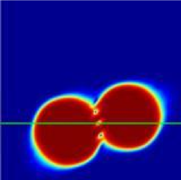
(a) Contours of $\Psi_{1}$

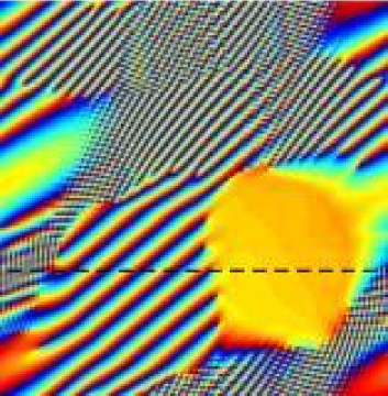
(b) Contours of $\Phi_{1}$

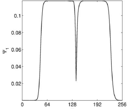
(c) Lineplot of $\Psi_{1}$ along solid line in (a)

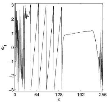
(d) Lineplot of $\Phi_{1}$ along dashed line in (c)

Figure 3: (Color online) (a) and (c): The field $\Psi_{1}$, smooth everywhere except near interfaces and defects. (b) and (d) The field $\Phi_{1}$, which is computed naively as $\arctan(\Im(A_{1})/\Re(A_{1}))$ is periodic and discontinuous. The chaotic fluctuations in $\Phi_{1}$ in the regions outside the crystals correspond to the liquid phase where $\Phi_{1}$ has no physical meaning. The rapid, but periodic, variations of $\Phi_{1}$ in the left grain is due to its large misorientation angle of $\pi/6$. In contrast, the grain on the right is oriented along $\mathbf{k}_{j}$ causing $\Phi_{1}$ to vary much more smoothly.

The field $\Psi_{j}$ is nearly constant within the individual grains and varies sharply only near grain boundaries, rendering its equation ideally suited for solution on adaptive meshes. The field $\Phi_{j}$ on the other hand, if computed naively as $\arctan(\Im(A_{j})/\Re(A_{j}))$, is a periodic and discontinuous function bounded between the values $-\pi$ and $\pi$, with a frequency that increases with increasing grain misorientation. This poses a problem similar to that previously posed by the beats, with the grid this time having to resolve the fine scale structure of $\Phi_{j}$. Further, one may need to resort to shock-capturing methods in order to correctly evaluate higher order derivatives, and resolve jumps where $\Phi_{j}$ changes value from $\pi$ to $-\pi$ and vice-versa. Complications are also caused by $\Phi_{j}$ being undefined in the liquid phase, and the tendency for $\Psi_{j}$, which appears in the denominator on the right hand side of Eq. (14), to approach zero at those locations. This calls for some type of robust regularization scheme for the phase equations. These problems are clearly highlighted in Fig. 3, which shows the impingement of two misaligned crystals and the corresponding values of $\Psi_{1}$ and $\Phi_{1}$.

Ideally, one would like to reconstruct from the periodic $\Phi_{j}$, a continuous surface $\Phi_{j}+2n\pi$ (where $n$ is an integer) which would be devoid of jumps, and therefore amenable to straightforward resolution on adaptive meshes. The implementation of such a reconstruction algorithm however, even if possible, requires information about individual crystal orientations, and the precise location of solid/liquid interfaces, defects, and grain boundaries at every time step, making it very computationally intensive. Further, such an algorithm would be more appropriate in the framework of an interface-tracking approach such as the level set method Sethian (1996), rather than our phase-field modeling approach.

Despite these issues with the polar (phase/amplitude) equations progress can be made, under certain non-critical approximations, by solving the phase/amplitude equations in the interior of crystalline regions, in conjunction with the Cartesian complex amplitude equations in regions closer to domain boundaries and topological defects.

III.2 Reduced equations and the frozen phase gradient approximation

The main idea that will be developed in this and subsequent sections is that of evolving the phase/amplitude and complex amplitude equations simultaneously in different parts of the domain, depending on where they can most appropriately be applied. The phase/amplitude formulation is solved in the crystal interior, away from defects, interfacial regions, and the liquid phase. The complex amplitude equations are solved everywhere else in the computational domain. This does away with the need for regularizing the phase equations where $\Psi_{j}\to 0$ (since $\Psi_{j}\gg 0$ in the crystal interior) as well as the issue of the phase being undefined in certain regions. We overcome the remaining issues with the phase equation, i.e. the difficulty of evaluating derivatives of the phase and the need to resolve its periodic variations via certain controlled approximations described next.

Let us examine the results of a fixed grid calculation performed using the complex amplitude equations, illustrated in Fig. 4, showing a sequence of line plots of the quantity $\Delta(\partial\Phi_{1}/\partial x)=\left.\partial\Phi_{1}/\partial x\right|_{t=840}-\left.\partial\Phi_{1}/\partial x\right|_{t}$. $\nabla\Phi_{j}$ inside the growing crystal is seen to be essentially time invariant. As the crystal on the left grows, it can be seen that $\Delta(\partial\Phi_{1}/\partial x)$ stays close to zero inside. We have verified that this is also true for the $y$ component of $\nabla\Phi_{1}$, and both components of $\nabla\Phi_{2}$ and $\nabla\Phi_{3}$.

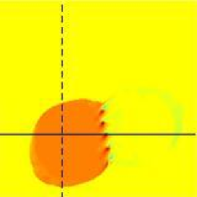
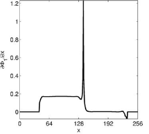
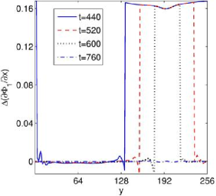
(a)	(b)	(c)

Figure 4: (Color online) $\Phi_{1}$ and its time evolution for the pair of crystals shown in Fig. 3. (a) Contours of $\partial\Phi_{1}/\partial x$ at $t=520$. (b) Lineplot of $\partial\Phi_{1}/\partial x$ along solid line in (a). (c) $\Delta(\partial\Phi_{1}/\partial x)$ along dashed line in (a). Just as with $\Psi_{j}$, the components of $\nabla\Phi_{j}$ are also practically constant inside the individual crystals. The spike in (b) corresponds to a defect on the grain boundary. As seen from the time series in (c) for $\partial\Phi_{1}/\partial x$, $\nabla\Phi_{j}$ hardly changes in the crystal bulk during its evolution.

These results suggest that we may employ a locally frozen phase gradient. Note that the assumption of a frozen phase gradient does not mean that $\Phi_{j}$ itself cannot change. $\Phi_{j}$ can continue to evolve as per Eq. (17) under the constraint of a fixed $\nabla\Phi_{j}$, although the changes may actually be quite small. On the other hand, when similarly oriented crystals collide to form a small angle grain boundary, it is energetically more favorable for grains to locally realign (i.e. for $\nabla\Phi_{j}$ to change close to grain boundaries) in order to reduce orientational mismatch Harris et al. (1998); Moldovan et al. (2002a, b, c), rather than to nucleate dislocations. Since such interaction effects originate at the grain boundary, where the full complex RG equations will be solved, we anticipate that our assumption will not lead to artificially “stiff” grains.

This approximation allows us to neglect third and higher order derivatives of $\Psi_{j}$ and $\Phi_{j}$ , which allows us to reduce Eqs. (13) and (14) to the following second order PDEs:

$$\frac{\partial\Psi_{j}}{\partial t} = (r+3\bar{\psi}^{2})\left[-\Psi_{j}+\mathcal{C}^{\Re}(\Psi_{j},\Phi_{j})\right]$$ (16)

$$-3\Psi_{j}\left(\Psi_{j}^{2}+2\sum_{k\neq j}\Psi_{k}^{2}\right)-6\frac{\bar{\psi}}{\Psi_{j}}\left(\prod_{k}\Psi_{k}\right)\cos\left(\sum_{k}\Phi_{k}\right)$$

$$\frac{\partial\Phi_{j}}{\partial t} = \frac{(r+3\bar{\psi}^{2})\mathcal{C}^{\Im}(\Psi_{j},\Phi_{j})}{\Psi_{j}}+6\frac{\bar{\psi}}{\Psi_{j}^{2}}\left(\prod_{k}\Psi_{k}\right)\sin\left(\sum_{k}\Phi_{k}\right),$$ (17)

where $\mathcal{C}^{\Re}$ and $\mathcal{C}^{\Im}$ contain only first and second order derivatives of $\Psi_{j}$ and $\Phi_{j}$. Eqs. (16) and (17) are referred to as the reduced phase/amplitude equations.

The task of evolving the phase/amplitude equations is now considerably simplified, as only derivatives up to second order in $\Phi_{j}$ need to be computed. While the Laplacian and gradient of $\Psi_{j}$ can be computed in a straightforward manner using Eqs. (27) and (31) respectively, the gradient of $\Phi_{j}$ needs to be computed with a little more care (in order to avoid performing derivative operations on a discontinuous function). The result is that

$$\nabla\Phi_{j}=\frac{\Re(A_{j})\nabla\Im(A_{j})-\Im(A_{j})\nabla\Re(A_{j})}{\Psi_{j}^{2}}.$$ (18)

Thus, the gradient operation on a discontinuous function $\Phi_{j}$ is now transformed into gradient operations on the smooth components of the complex amplitude $A_{j}$. Further, $\nabla^{2}\Phi_{j}$ is computed as $\nabla\cdot\nabla\Phi_{j}$, where the divergence operator is discretized using a simple second order central difference scheme.

However, as can be seen from Eq. (18), $\nabla\Phi_{j}$ now depends on gradients of the real and imaginary components of $A_{j}$, which may not be properly resolved in the crystal bulk as we intend to coarsen the mesh there. To address this point, we assume that $\nabla\Phi_{j}$ is frozen temporally in the crystal bulk. This assumption implies that once $\nabla\Phi_{j}$ is accurately initialized in the crystal interior via Eq. (18), after ensuring adequate resolution of the components of $A_{j}$, it need not be computed again. For example, in simulations of crystal growth from seeds, we can start with a mesh that is initially completely refined inside the seeds, so that $\nabla\Phi_{j}$ is correctly computed. Once initial transients disappear and the crystals reach steady state evolution, the growth is monotonic in the outward direction. From this point on, $\nabla\Phi_{j}$ hardly changes inside the crystal bulk and the grid can unrefine inside the grains while correctly preserving gradients in $\nabla\Phi_{j}$. Note that the apparent discontinuities in $\Phi_{j}$ no longer need be resolved by the grid.

IV A hybrid formulation

In order to implement our idea of evolving Eq. (7), and Eqs. (16) and (17) selectively within different regions, we begin by dividing the computational domain into two regions where each set of equations may be evolved simultaneously in a stable fashion. The region where $A_{j}$ is computed in terms of its real and imaginary parts is called X, and the region where $\Psi_{j}$ and $\Phi_{j}$ are computed is called P. We ensure that subdomain P is well separated from locations with sharp gradients, such as interfaces and defects. Otherwise, errors resulting from our approximations may grow rapidly, causing X to invade P, which will in turn require us to solve the complex equations everywhere. We will further assume that the decomposition algorithm is implemented after a sufficient time, when initial transients have passed, and that the crystals are evolving steadily, which implies that $\Psi_{j}$ inside the crystals has reached some maximum saturation value $\Psi_{j}^{max}$. The scenario we have in mind is sketched in Fig. 5, with P constituting the shaded regions and all other regions correspond to X.

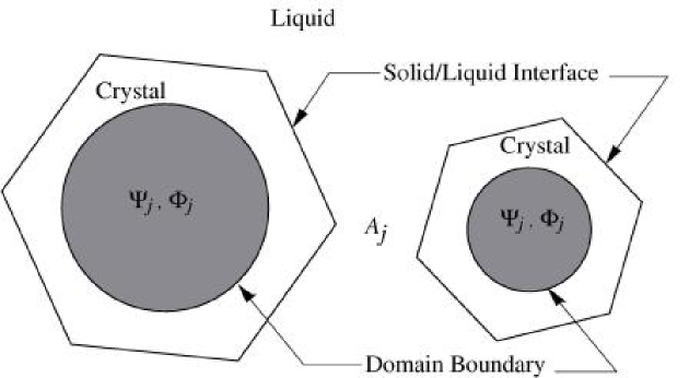
Figure 5: Sketch illustrating the idea of selectively evolving the complex amplitude and phase/amplitude equations in different regions of the computational domain. $\Psi_{j}$ and $\Phi_{j}$ are evolved inside the shaded circles, which fall well inside the crystalline phase, while the real and imaginary components of $A_{j}$ are evolved everywhere else.

The pseudo-code shown in Algorithm 1 presents a simple algorithm to achieve this decomposition. The algorithm first determines nodes with $\Psi_{j}$ exceeding some minimum value $\gamma\Psi_{j}^{max}$, and $|\nabla\Psi_{j}|$ beneath some limit $\epsilon_{1}$. The nodes satisfying these conditions constitute domain P, while those failing to, constitute X. The P nodes are then checked again to see if the quantity $|\nabla(|\nabla\Phi_{j}|)|$ is under some limit $\epsilon_{2}$. Nodes in set P that fail to satisfy this condition are placed in set X. The parameters $\gamma$, $\epsilon_{1}$, and $\epsilon_{2}$ are chosen to ensure the largest possible size of set P. A small problem is caused by the fields $\Psi_{j}$ and $|\nabla\Phi_{j}|$ not being perfectly monotonic. As the limits $\epsilon_{1}$ and $\epsilon_{2}$ are sharp, several small islands (clusters of grid points) of X or P can be produced, which are detrimental to numerical stability. We have resolved this issue via a coarsening algorithm that eliminates very small clusters of X and P.

Algorithm 1 (Color online) Domain decomposition. The parameters $\gamma$, $\epsilon_{1}$, and $\epsilon_{2}$ are heuristic.

  Compute $\Psi_{j}^{max}$

  $\Psi_{j}^{max}=\gamma\times\Psi_{j}^{max}$

  {Split domain based on the magnitude of $\Psi_{j}$ and $|\nabla\Psi_{j}|$}

  for i = 1 to maxnode do {loop over all nodes}

     count = 0

     for j = 1 to 3 do {loop over amplitude components}

        if $\Psi_{j}\geq\Psi_{j}^{max}$ and $|\nabla\Psi_{j}|\leq\epsilon_{1}$ then

           count++

        end if

     end for

     if count = 3 then

        domain = P {passed test, solve phase/amplitude equations}

     else

        domain = X {failed test, solve complex equations}

     end if

  end for

  {Split domain based on $\left|\nabla\left(|\nabla\Phi_{j}|\right)\right|$}

  for i = 1 to maxnode do {loop over all nodes}

     count = 0

     if domain = P then {check only nodes that passed previous test}

        for j = 1 to 3 do {loop over amplitude components}

           if $|\nabla(|\nabla\Phi_{j}|)|\leq\epsilon_{2}$ then

              count++

           end if

        end for

        if count $\neq$ 3 then

           domain = X {failed test, solve complex equations}

        end if

     end if

  end for

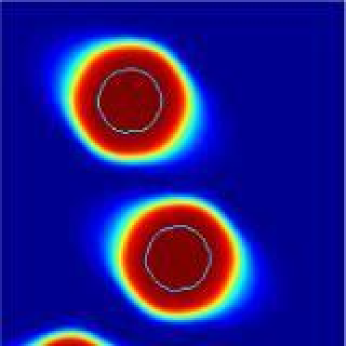
(a) $t=120$

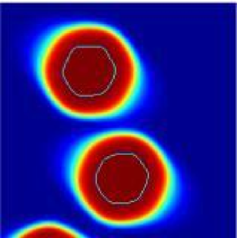
(b) $t=200$

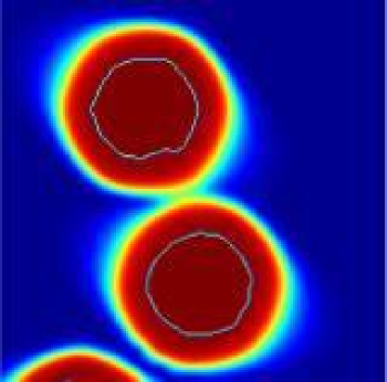
(c) $t=280$

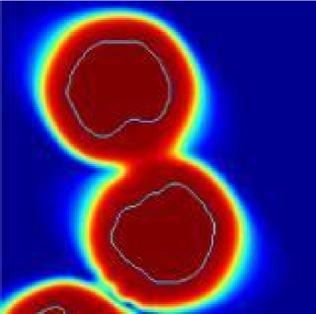
(d) $t=360$

Figure 6: (Color online) Filled contour plot showing the time evolution of three misoriented crystals. The field plotted is $\Psi_{3}$. Superimposed on the plot as solid curves are the boundaries that separate domains X and P, with P being enclosed by the curves.

Fig. 6 shows results from a uniform grid implementation of Algorithm 1. No islands are present, as the algorithm decomposes the domain in an unsupervised manner. It is noteworthy that domain boundaries are distorted in Figs. 6(c) and 6(d) in response to the formation of a grain boundary between the two crystals, after being roughly hexagonal at earlier times. The fact that the domain separatrices maintain a safe distance from the grain boundary ensures that the phase/amplitude equations are not evolved in regions containing sharp gradients in $\nabla\Phi_{j}$. Parameter values used were $\gamma=0.85$, $\epsilon_{1}=0.0005$, and $\epsilon_{2}=0.003$.

The remarkable feature of our numerical scheme is that solving different sets of equations in X and P does not require doing anything special near the domain boundaries, such as creating “ghost” nodes outside each domain, or constraining solutions to match at the boundaries. Both sets of variables, {$\Psi_{j},\Phi_{j}$} and {$A_{j}$}, are maintained at all grid points irrespective of the domain they belong to, with one set allowing easy computation of the other . Therefore the transition between the two domains is a continuous one in terms of field variables, which allows the finite difference stencils in Eqs. (27) and (31) to be applied to the respective fields without any modification near domain boundaries.

V Solving the RG Equations with Adaptive Mesh Refinement

As highlighted in earlier work Provatas et al. (1998b); Provatas et al. (1999); Jeong et al. (2003, 2001) the use of dynamic adaptive mesh refinement alters the numerical mesh resolution dynamically such as to place high resolution near phase boundaries and a very low resolution in bulk regions where there is little activity. This dramatically reduces computer memory requirements, allowing larger systems to be simulated. It also significantly reduces overall simulation times. The determining factor guiding the use or otherwise of an AMR technique to solve a particular problem is the simple criterion

$$\frac{{\rm Interface\,length\,(orArea)}}{{\rm Domain\,area\,(orVolume)}}\ll 1$$ (19)

The phase/amplitude RG equations discussed above are precisely in the class of problems that can benefit from and is amenable to adaptive mesh refinement. Indeed, as will be shown below, the speedup in time contained intrinsically by the physics of the PFC equation is complemented by the concomitant bridging of length scales afforded by the RG equations solved adaptively.

We solved the RG equations discussed above using a new C++ adaptive mesh refinement (AMR) algorithm that uses finite differences (FD) to resolve spatial gradients J. Fan and Provatas (2006). While it is typical to use the finite element method (FEM) in situations involving non-structured meshes, adaption using finite differences schemes allows approximately a 5-10 fold increase in simulation speed (measured as CPU time per node) over previous (FEM) formulations involving traditional phase field models Provatas et al. (1998b); Provatas et al. (1999). This improvement increases further still in cases where model equations contain spatial gradients or order higher than two, such as in the case of Eqs. (7), (16) and (17). The basic reason for the difference in speeds is that FEM formulations generally have more overhead due to their reliance on local matrix multiplication at multiple Gauss quadrature points. This overhead time becomes even more pronounced when using elements of order higher than two, as is required if an FEM formulation is to be used to resolve the spatial derivatives involved with the RG equations in this work.

V.1 AMR Algorithm

At the heart of our algorithm is a routine that creates a non-uniform mesh that increases nodal density in specific regions according to a local error estimator. Nodes are grouped into pseudo-elements, managed by dynamic tree data structures, as used in a finite element formulation by Provatas et al Provatas et al. (1999). The quad-tree structure illustrated in Figure 7 is a hierarchy of elements where every level deeper in the tree results in elements of higher refinement. Every element has associated with it 4 corner ‘nodes’ and 5 ‘ghost’ nodes: 4 in the center of each edge and 1 in the center of the element. The ghost nodes facilitate interpolation when neighboring elements are at different levels of refinement. Each node is a structure containing field values, such as phase, amplitude and the real and complex components of $A_{j}$. A node also contains information about its nearest neighbors. Edge ghost nodes can serve as field nodes if a resolution mismatch occurs across neighbor elements. This can be seen in the schematic in figure 7. The field equations are not solved at ghost nodes, but are instead interpolated linearly from the nodal values of the element (or edge) to which they belong. The inclusion of ghosts nodes simplifies the calculation of local derivatives.

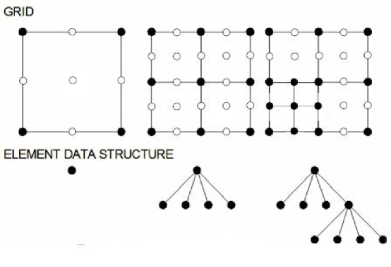
Figure 7: Schematic of a quad-tree data structure used in adaptive meshing. An element splits and creates ’children’ beneath it in the tree structure. Nodes are created at the corner of each element and ’ghost’ nodes are placed in the center of elements and along edges that have no real nodes, to accommodate resolution mismatches. Ghost nodes are approximated by interpolation from the element to which they belong.

An adapter algorithm refines/unrefines the tree structure by using a user-defined error estimator computed for each element. Refinement is done by bisection as shown in Figure 7, and unrefinement is done by fusing four child elements into their parent element. Once refinement/unrefinement of all elements is complete, the adapter produces an array of nodes, each of which is the center of a local grid. The equation solver accepts this array as input and then solves the equations at these nodal points. This method of node organization modularizes our algorithm and allows the solver and adapter to be separately parallelized.

The mesh data structure contains nodes with detailed knowledge of their local neighbors, each of which exist at the center of a $5\times 5$ uniform mesh (See Fig. 8). During adaptation, the data structure applies rules that either increase (if higher accuracy is needed) or decrease (to decrease memory requirements) the size of this local nodal mesh. Also during adaptation, the data structure and its associated elements and nodes respect the following six rules (3 applied to each element and 3 to each node). Rule 1 ensures mesh cohesion and maintains accuracy in the solution of the PDEs.

RULE 1:

Neighboring elements can vary by at most one level

RULE 2:

All elements contain 9 nodes, real or ghost

RULE 3:

Element neighbors are all at the same level (Therefore elements may have $NULL$ as a neighbor)

RULE 4:

Node neighbors are all at the same level (Nodes will never have $NULL$ as a neighbor, but may instead have a ghost as a neighbor)

RULE 5:

Each node is at the center of what is defined as a uniform mini-mesh

RULE 6:

Each node is assigned the resolution ($\Delta x$) of the most refined element attached to it.

The adaptive process is controlled primarily at the tree level, but invokes function calls inside of the element and node structures. Its basic flow is illustrated in Algorithm 2. This process allows an element-by-element examination using recursion to maintain the rules above. Once the process of adaptation is complete the adapter creates an array of nodes each with the index of its neighbors in the array, which is then used to solve the equations before adapting again. We also note that element ‘leaves’ are stored by their resolution level in an array of element lists. Element resolution is restricted to vary by at most one level compared to the element neighbors (Rule 1).

Algorithm 2 Regridding algorithm

  Delete the Ghost Pointer List

  while Some elements have split or unsplit do

     Check all elements for unsplitting criteria

     Check all elements for splitting criteria

  end while

  Update node neighbors

  Build Ghost List

  Set Ghost Averaging Information

Element splitting (refinement) is the dominant process in the algorithm, taking precedence over element coarsening (i.e. fusing four children elements into their parent). Elements are searched one refinement level at a time, starting from the second highest level of resolution. Each element is considered for splitting using an error criterion computed for that element. If splitting is required, an element data structure it is pushed onto a stack, where its neighbors are subsequently checked against Rule 1. If splitting will violate Rule 1, the neighbors are recursively split until all refined elements satisfy Rule 1. When an element is split, it and its updated neighbor elements generate new real and ghost nodes, as well as information about their neighbors. The splitting algorithm is illustrated in Algorithm 3.

Algorithm 3 Splitting Algorithm

  for ElementLevel=maxLevel-1 to 0 do

     while Level is not empty do

        if Element Splitting criteria is met then

           PUSH Element onto stack

           while Stack is not empty do

              if Top of Stack’s neighbors need splitting then

                 Push Needed neighbors onto stack

              else

                 Pop the Element from the Stack

                 Create 4 new children elements

                 Push children onto ElementLevel+1

                 Add New Nodes to the Node List

                 Remove former Ghosts from Ghost List

              end if

           end while

        end if

     end while

  end for

The unrefinement algorithm starts at the lowest level of refinement. Again, Rule 1 above must be imposed. The elements are examined to see if a parent requires splitting. If it does not, the parent has its four child elements eliminated, assuming their relationship with the neighbors allows it (i.e. Rule 1). Recursive unsplitting of elements is not allowed. As in the case of refinement, during unrefinement, element neighbors and node neighbors are updated. The flow of unsplitting is shown in Algorithm 4.

Algorithm 4 UnSplitting Algorithm

  for ElementLevel=maxLevel-1 to 0 do

     while Level is not empty do

        if Element Splitting criteria is NOT met then

           if Element’s Parent’s Splitting criteria is NOT met then

              if Parent’s Children Have NO Children then

                 if Parent’s neighbor’s are Same level or One level Lower then

                    ADD Parent to ElementLevel+1

                    REMOVE Parent’s Children from ElementLevel

                    REMOVE Unneeded nodes from node list

                    REMOVE Ghosts from Ghost list

                    Center Node Becomes a Ghost

                    Edge Nodes Become Ghosts depending on neighbor levels

                    DELETE Children

                 end if

              end if

           end if

        end if

     end while

  end for

As discussed above, nodes follow rules 4, 5 and 6. This is enforced by the introduction of ghost nodes in elements and by maintaining rule 1. Rule 5 is maintained by creating a list of local nodes (ghost or real) and by maintaining rule 1 during splitting. Rule 6 determines which node neighbors are chosen and the local node spacing ($\Delta x$). A real node will contain the minimesh on which is applied the governing equations; a ghost node provides instructions on how to interpolate the values needed for real node calculations.

V.2 Handling of Ghost Nodes in The Hybrid Formulation

A very useful feature of the AMR implementation outlined in the previous section is that each node sits at the center of a uniform $5\times 5$ mini-grid, illustrated in Fig. 8. Let us focus on the node represented by the lightly shaded circle (labeled F). The data structure ensures that node F has access to all other nodes on the wireframe. The advantage of this construction is that it allows us to use the uniform grid finite difference stencils for the Laplacian and gradient operators in Eqs. (27) and (31) respectively, instead of modifying them node-wise to accommodate variations in grid spacing. This requires the introduction of ghost nodes, shown as open circles in Figure 8.

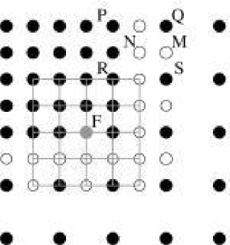
Figure 8: Schematic showing a portion of the adaptive grid where the refinement level changes. Filled circles (and node F) are real nodes where the fields are computed, whereas the open circles are non-computational ghost nodes where the fields are interpolated.

The scheme used to interpolate values at the ghost nodes is a potential source of error in the numerical solution, and must be chosen carefully. $\Psi_{j}$, $\partial\Phi_{j}/\partial x$, $\partial\Phi_{j}/\partial y$, $\Re(A_{j})$ and $\Im(A_{j})$ are very smoothly varying functions, and therefore we linearly interpolate their values to the ghost nodes. Values at ghosts residing on element edges, for example node M in Fig. 8, are obtained by averaging values of the two end nodes Q and S, whereas values at ghosts residing at the center of an element, node N for example, are obtained by averaging the values at the four corner nodes, P, Q, R, and S. We have found this interpolation scheme to be quite stable. We note however that, given the near-periodic variations in $\Re(A_{j})$ and $\Im(A_{j})$, especially in misoriented grains, higher order interpolation functions (such as cubic splines) could improve solution accuracy, while strongly enforcing continuity of fields across elements. This issue will be examined in future work.

The interpolation of $\Phi_{j}$ at the ghost nodes is a little more delicate. Since $\Phi_{j}$ is a discontinuous function, a simple average of the values at the neighboring real nodes may not always give the correct answer, especially because the grid does not resolve the discontinuities. Even if it did, a simple average could lead to the wrong result. As an example, consider the two real nodes Q and S in Fig. 8, with values $\Phi_{1}^{Q}=\pi-\delta_{1}$ and $\Phi_{1}^{S}=-\pi+\delta_{2}$ where $\delta_{1}$ and $\delta_{2}$ are very small but positive real numbers, on either side of a discontinuity in $\Phi_{1}$. We wish to determine the value at the ghost node M that lies between Q and S. Although the values of $\Phi_{1}$ at Q and S are essentially equivalent in phase space, differing in magnitude by approximately $2\pi$, a simple average gives $\Phi_{1}^{M}=(\delta_{2}-\delta_{1})/2\approx 0$, which is quite wrong.

In order to interpolate correctly we need to make use of $\nabla\Phi_{j}$. For example in the above case, the total change in the phase from Q to S is obtained by integrating the directional derivative of $\Phi_{1}$ along the edge QS, i.e.

$$\Delta\Phi_{1}^{QS}=\int_{Q}^{S}\nabla\Phi_{1}\cdot d\mathbf{r}=\int_{y=y^{Q}}^{y^{S}}\frac{\partial\Phi_{1}}{\partial y}dy.$$ (20)

Eq. (20) can be evaluated numerically, and the accuracy of the result depends on how well $\partial\Phi_{1}/\partial y$ is approximated. Consistent with our earlier assumptions, we approximate $\partial\Phi_{1}/\partial y$ as piecewise constant where

$$\frac{\partial\Phi_{1}}{\partial y}=\frac{1}{2}\left(\left.\frac{\partial\Phi_{1}}{\partial y}\right|_{S}+\left.\frac{\partial\Phi_{1}}{\partial y}\right|_{Q}\right)$$ (21)

which leads to

$$\Delta\Phi_{1}^{QS}=\frac{1}{2}\left(\left.\frac{\partial\Phi_{1}}{\partial y}\right|_{S}+\left.\frac{\partial\Phi_{1}}{\partial y}\right|_{Q}\right)\left(y^{S}-y^{Q}\right).$$ (22)

Since $\partial\Phi_{1}/\partial y$ is constant along the edge QS, $\Phi_{1}$ must vary linearly along QS. Hence at node M,

$$\Phi_{1}^{M}=\Phi_{1}^{S}+\frac{1}{2}\Delta\Phi_{1}^{QS}\;:\;\Phi_{1}^{M}\in[-\pi,\pi].$$ (23)

Interpolation of $\Phi_{j}$ at element center ghost nodes, such as N, is done in a similar manner by interpolating linearly from ghost nodes at the centers of opposite element edges. Once again, this scheme might be improved by choosing higher order polynomials to approximate $\nabla\Phi_{j}$ inside elements.

V.3 Refinement Criteria in the Hybrid Formulation

Traditionally, AMR algorithms rely on some kind of local error estimation procedure to provide a criterion for grid refinement. Zienkiewicz and Zhu Zienkiewicz and Zhu (1987) developed a simple scheme for finite element discretization of elliptic and parabolic PDEs by computing the error in the gradients of the fields using higher order interpolation functions. Berger and Oliger Berger and Oliger (1984) on the other hand estimated the local truncation error of their finite difference discretization of hyperbolic PDEs via Richardson extrapolation. Depending on the equations being solved and the numerical methods being used, one scheme may be more effective than another. We use a very simple and computationally inexpensive refinement criterion that works nicely for our equations, based purely on gradients in the various fields.

The outline of the algorithm used to decide whether or not to split an element is given in Algorithm 5. The algorithm initially computes absolute changes in the real and imaginary parts of $A_{j}$, and the $x$ and $y$ components of $\nabla\Phi_{j}$ in each element. We use absolute differences in place of derivatives in order for the refinement criterion to be independent of element size. We note that prior to implementing this algorithm, the domain decomposition algorithm described above (see Figure 1) needs to be called first in order to split the computational domain into subdomains X and P.

The process begins by examining an element flag to see if the element lies on the separatrix between X and P, or in $k$ layers from the boundary, within the P subdomain. If so this element is split. This ensures that the fields are always resolved on the interface between X and P, and just within the boundary on the P side. The latter is required because of the higher order derivative operations that need to be performed while evolving the complex amplitude equations in X.

Algorithm 5 Criteria for element splitting

  {N1, N2, N3 and N4 are the element nodes in clockwise manner}

  for i = 1 to 3 do {loop over amplitude components}

     {Change in real part of $A_{i}$ over element}

     $DR_{i}=|\mbox{N1}\rightarrow\Re(A_{i})-\mbox{N2}\rightarrow\Re(A_{i})|+|\mbox{N2}\rightarrow\Re(A_{i})-\mbox{N3}\rightarrow\Re(A_{i})|$

     $+|\mbox{N3}\rightarrow\Re(A_{i})-\mbox{N4}\rightarrow\Re(A_{i})|+|\mbox{N4}\rightarrow\Re(A_{i})-\mbox{N1}\rightarrow\Re(A_{i})|$

     {Change in imaginary part of $A_{i}$ over element}

     $DI_{i}=|\mbox{N1}\rightarrow\Im(A_{i})-\mbox{N2}\rightarrow\Im(A_{i})|+|\mbox{N2}\rightarrow\Im(A_{i})-\mbox{N3}\rightarrow\Im(A_{i})|$

     $+|\mbox{N3}\rightarrow\Im(A_{i})-\mbox{N4}\rightarrow\Im(A_{i})|+|\mbox{N4}\rightarrow\Im(A_{i})-\mbox{N1}\rightarrow\Im(A_{i})|$

     {Change in $x$ component of $\nabla\Phi_{i}$ over element}

     $DGPX_{i}=|\mbox{N1}\rightarrow\partial\Phi_{1}/\partial x-\mbox{N2}\rightarrow\partial\Phi_{1}/\partial x|+|\mbox{N2}\rightarrow\partial\Phi_{1}/\partial x-\mbox{N3}\rightarrow\partial\Phi_{1}/\partial x|$

     $+|\mbox{N3}\rightarrow\partial\Phi_{1}/\partial x-\mbox{N4}\rightarrow\partial\Phi_{1}/\partial x|+|\mbox{N4}\rightarrow\partial\Phi_{1}/\partial x-\mbox{N1}\rightarrow\partial\Phi_{1}/\partial x|$

     {Change in $y$ component of $\nabla\Phi_{i}$ over element}

     $DGPY_{i}=|\mbox{N1}\rightarrow\partial\Phi_{1}/\partial y-\mbox{N2}\rightarrow\partial\Phi_{1}/\partial y|+|\mbox{N2}\rightarrow\partial\Phi_{1}/\partial y-\mbox{N3}\rightarrow\partial\Phi_{1}/\partial y|$

     $+|\mbox{N3}\rightarrow\partial\Phi_{1}/\partial y-\mbox{N4}\rightarrow\partial\Phi_{1}/\partial y|+|\mbox{N4}\rightarrow\partial\Phi_{1}/\partial y-\mbox{N1}\rightarrow\partial\Phi_{1}/\partial y|$

  end for

  if element on X/P boundary OR k layers inside P then

     Split element and exit

  else if element inside X then

     count=0

     for i = 1 to 3 do {loop over amplitude components}

        if $DR_{i}\geq\epsilon_{1}$ OR $DI_{i}\geq\epsilon_{1}$ then

           count++

        end if

     end for

     if count $\neq$ 0 then

        Split element and exit

     end if

  else {element is inside P}

     count = 0

     for i = 1 to 3 do {loop over amplitude components}

        if $DGPX_{i}\geq\epsilon_{2}$ OR $DGPY_{i}\geq\epsilon_{2}$ then

           count++

        end if

     end for

     if count $\neq$ 0 then

        Split element and exit

     end if

  end if

If the element does not split and belongs to X (where $A_{j}$ are the field variables), the variations in the real and imaginary parts of $A_{j}$ are checked to see if they exceed a certain bound $\epsilon_{1}$. If any one of them does, this element is split. If, on the other hand, the element belongs to P where the phase/amplitude equations are solved, variations in the $x$ and $y$ components of $\nabla\Phi_{j}$ are checked to see if they exceed another limit $\epsilon_{2}$. If they do, this element is split. If none of the above criteria are satisfied, the element is not split and is placed in the list of elements to be checked for coarsening. Since refinement criteria are recursively applied to the quadtree, the finest elements are automatically placed around domain separatrices, solid/liquid interfaces, and defects.

VI Results and computational efficiency

Using the various approximations and algorithms described in the previous sections we solved the phase/amplitude and complex equations simultaneously in different parts of our computational domain using adaptive mesh refinement. Algorithm 6 shows the flow of control in the main routine. The complex amplitude equations, Eq. (7), are initially evolved everywhere until time $N_{tr}$, when initial transients have dissipated, and the crystals evolve steadily outward. The domain is then split into subdomains X and P, following which the reduced phase/amplitude equations, Eqs. (16) and (17), are evolved using a forward Euler time stepping scheme in subdomain P. The grid is refined after a predetermined number of time steps $N_{adapt}$, which is chosen heuristically. We note that the current implementation can handle only periodic boundary conditions. Work is currently underway to enable handling of more general boundary conditions.

Algorithm 6 Flow of control

  InitVar() {Initialize program variables and parameters}

  InitGrid() {decide where to initially refine/coarsen based on initial condition}

  UpdateGhostsFV() {interpolate $A_{j}$, $\Psi_{j}$, $\Phi_{j}$ at ghost nodes}

  ComputePhaseGradients(1) {compute $\nabla\Phi_{j}$ everywhere}

  UpdateGhostsPG() {interpolate $\nabla\Phi_{j}$ at ghost nodes}

  for i = 1 to $N_{tr}-1$ do {evolve until initial transients subside}

     if i $\bmod$ $N_{adapt}$ = 0 OR i = 1 then

        AdaptGrid() {uses Algorithm 5}

     end if

     EvolveComplexAmp() {evolve Eq. (7) everywhere}

     UpdateAllFields() {compute $\Psi_{j}$ and $\Phi_{j}$ from $A_{j}$}

     UpdateGhostsFV()

     ComputePhaseGradients(1)

     UpdateGhostsPG()

  end for

  DivideDomain() {call Algorithm 1 to split domain into X and P}

  for i = $N_{tr}$ to $N_{end}$ do {evolve after transients subside}

     if i $\bmod$ $N_{adapt}$ = 0 then

        DivideDomain()

        AdaptGrid()

     end if

     EvolveComplexAmp() {evolve Eq. (7) in X}

     EvolvePhaseAmp() {evolve Eqs. (16) and (17) in P}

     UpdateAllFields() {evaluate $\Psi_{j}$ and $\Phi_{j}$ in X, evaluate $A_{j}$ in P}

     UpdateGhostsFV()

     ComputePhaseGradients(i) {compute $\nabla\Phi_{j}$ in X only, frozen gradient approx.}

     UpdateGhostsPG()

  end for

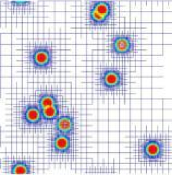
(a) t=0

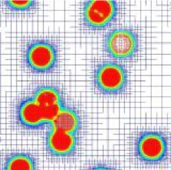
(b) t=88

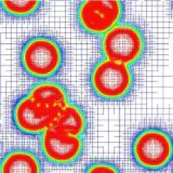
(c) t=168

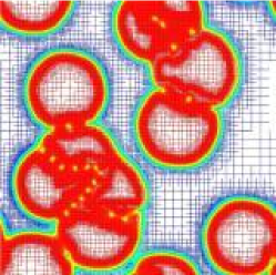
(d) t=248

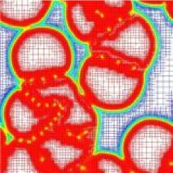
(e) t=320

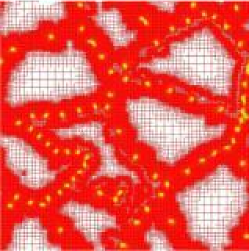
(f) t=552

Figure 9: (Color online) Evolution of a polycrystalline film simulated with Eq. (7), and Eqs. (16) and (17), using our adaptive mesh refinement algorithm. The conditions in this simulation are identical to those in section II.2 and Fig. 2. Note that the grid now coarsens inside grains that are misoriented with respect to $\mathbf{k}_{j}$, and “beats” are no longer a limitation. The colored field plotted is the average amplitude modulus, which is “red” inside the crystal phase, “blue” in the liquid phase, “green” at the crystal/liquid interface, and “yellow” near defects.

Using this implementation, we simulated the same problem (same initial and boundary conditions and problem parameters) that was solved adaptively in section II.2 using only the complex amplitude equations. Figure 9 shows the crystal boundaries and grid structure at various times during the simulation. $N_{tr}$ was chosen to be 3000 for this simulation. With $\Delta t=0.04$, this implies that this simulation is identical to the previous one until $t=N_{tr}\times\Delta t=120$. Thus, Figs. 9(a) and 9(b) are identical to Figs. 2(a) and 2(b). The advantage of the hybrid implementation starts to appear from Fig. 9(c), whenceforth, unlike in Fig. 2, even grains that are misoriented with respect to the basis $\mathbf{k}_{j}$ show grid unrefinement within. It is also noteworthy that the grid remains refined near solid/liquid interfaces, grain boundaries and defects, ensuring that key topological features are correctly resolved.

We now compare solutions from the two simulations quantitatively. We find it more informative to make a pointwise comparison of the two solutions along cross sections of the domain, rather than comparing solution norms, as we believe that this is a more stringent test of our implementation. We choose two random cuts, one running parallel to the $y$ axis at $x_{cut}=70\pi$, and the other parallel to the $x$ axis at $y_{cut}=118\pi$. The solutions are compared along these cuts at two different times, $t=168$ and $t=552$ in Figs. 10 and 11 respectively. The solid curves in the figures (labeled “hybrid”) are variations in $\Psi_{1}$ and $\partial\Phi_{1}/\partial x$ along the entire length of the domain as computed with the current (“hybrid”) implementation, whereas the symbols (labeled “complex”) are variations in the same variables as computed using fully complex equations (section II.2). The agreement is essentially perfect, indicating that our simplifications based on approximations in the preceding sections work reasonably well.

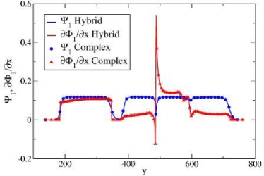
(a) $t=168$

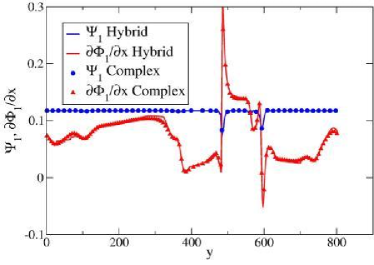
(b) $t=552$

Figure 10: (Color online) Numerical solution along the line $x=70\pi$ in Fig. 9 compared to the results using the hybrid scheme. Some of the data points in the complex solution were omitted for clarity of presentation.

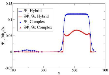
(a) $t=168$

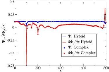
(b) $t=552$

Figure 11: (Color online) Numerical solution along the line $y=118\pi$ in Fig. 9 compared to the results using the hybrid scheme. Some of the data points in the complex solution were omitted for clarity of presentation.

Because the performance of our algorithm is sensitively tied to the type of problem that is being solved, it is difficult to come up with a simple metric that quantifies its computational efficiency. The difficulty lies in accounting for the change in CPU time per time step, which increases with the number of mesh points. For example, Fig. 12 shows the number of nodes in this simulation over time. Clearly, an adaptive grid implementation has a significant computational advantage over an equivalent fixed grid implementation at the early stages of the simulation.

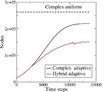
Figure 12: (Color online) Number of computational nodes in the grid as a function of time, for simulations in Fig. 2 (black curve) and Fig. 9 (red curve). The number of nodes reaches a constant value after all the liquid freezes. The dashed line shows the number of nodes required by a uniform grid implementation of the complex amplitude equations for the same problem.

One performance measure is the projected speed of our implementation compared to a uniform grid implementation of the PFC equation. This speedup is estimated by the simple formula,

$$S=\frac{N_{PFC}}{N_{RG-AG}}\times\frac{\Delta t_{RG-AG}}{\Delta t_{PFC}}\times\frac{1}{6}\times\beta$$ (24)

where $N_{PFC}$ is the number of grid points required to solve the PFC equation, $N_{RG-AG}$ is the number of grid points required in a hybrid implementation of the amplitude/RG equations, $\Delta t_{PFC}$ and $\Delta t_{RG-AG}$ are the time steps used in the respective implementations, the factor 1/6 comes from solving six RG equations in place of the [one] PFC equation directly, and $\beta\in[0,1]$ is the overhead of the AMR algorithm. The difficulty lies in fixing $N_{RG-AG}$ which is constantly changing with time. One estimate for $N_{RG-AG}$ is the number of nodes averaged over the entire simulation. This can be computed easily by dividing the area under the hybrid curve in Fig. 12 by the total number of time steps taken, which gives $N_{RG-AG}=104,747$. Further, based on heuristics collected while running our code, we conservatively estimate mesh refinement/coarsening to constitute about 3% of the CPU time, which gives $\beta=0.97$. Therefore, from Eq. (24) we have

$$S=\frac{1,050,625}{104,747}\times\frac{0.04}{0.008}\times\frac{1}{6}\times 0.97=8.1.$$ (25)

We do recognize that for a more accurate estimate of $S$ we would also need to consider overhead costs that may come from sub-optimal cache and memory usage owing to the data structures used. Hence these numbers should only be considered as rough estimates of true speedup.

While a speedup factor of 8 may not seem to be a great improvement in computational efficiency, one should bear in mind that the number of nodes in the AMR algorithm scales (roughly) linearly with interface/grain boundary length, which is quite substantial in the system we just simulated. Thus, one should not expect to derive the maximum computational benefit when simulating small systems with large numbers of grains. On the other hand, with this new method, we can now simulate the growth of a few crystals in a much larger system. We choose a square domain of side $4096\pi$, which in physical dimensions translates to 0.722 $\mu$m, if we assume an interatomic spacing of 4 Å . We initiate three randomly oriented crystals, two a little closer together than the third, so that a grain boundary forms quickly. The crystals are shown at different times in Fig. 13. The simulation was terminated at $t=3960$ when memory requirements exceeded 1 GB, after running on a dedicated 3.06 GHz Intel Xeon processor for about one week.

Let us calculate the speedup factor for this simulation as we did previously, after $70,000$ time steps ($t=2800$, Fig. 13(f)). Fig. 14 shows that the number of nodes in the adaptive grid varies nearly linearly with the number of time steps, and we estimate the average number of nodes $N_{AG-RG}$ to be $200,721$. The same simulation on a uniform grid using the PFC equation would have required $268,435,456$ nodes (not possible on our computers). We estimate $\beta=0.98$. In this case the speedup is about three orders of magnitude,

$$S=\frac{268,435,456}{200,721}\times\frac{0.04}{0.008}\times\frac{1}{6}\times 0.98=1091.$$ (26)

Fig. 15 shows vividly the range of length scales from nanometers to microns spanned by our grid in this simulation, highlighting its “multiscale” capability.

We would like to emphasize that as with any adaptive grid implementation, refinement criteria can change $S$ by a factor that is approximately constant. In order to enable testing our implementation on a much larger domain subject to the available memory resources, the criteria were relaxed. Note however, that even if we had roughly doubled the number of finely spaced nodes near the interfaces and the grain boundary, which would lead to a significantly more accurate calculation, $S$ would still be about 500 times faster than an equivalent implementation of the PFC equation on a uniform grid.

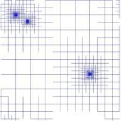
(a) t=0

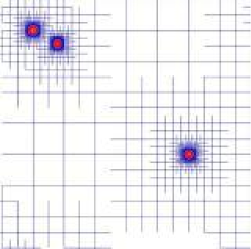
(b) t=840

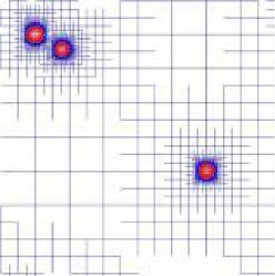
(c) t=1120

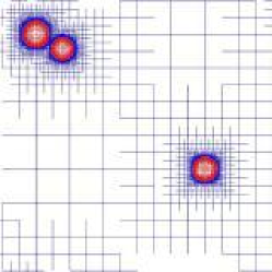
(d) t=1620

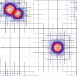
(e) t=2080

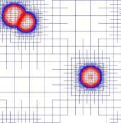
(f) t=2800

Figure 13: (Color online) Micro-scale simulation of two dimensional crystal growth with amplitude equations using AMR.

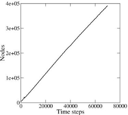
Figure 14: Number of computational nodes in the grid as a function of time for the 1 $\mu$m $\times$ 1$\mu$m domain. The growth is almost linear.

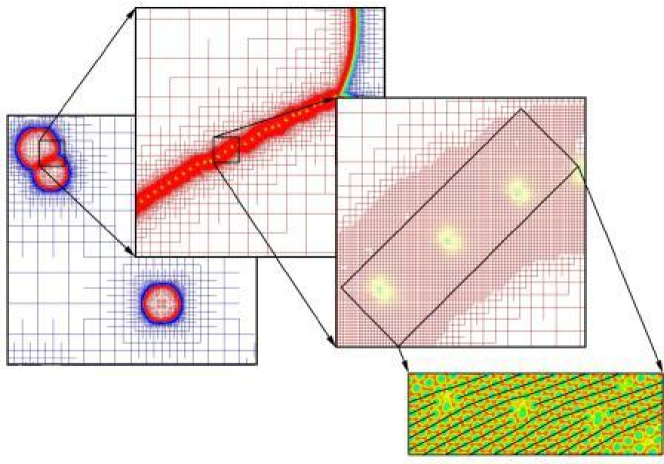
Figure 15: (Color online) The above grid spans roughly three orders of magnitude in length scales, from a nanometer up to a micron. The leftmost box resolves the entire computational domain whereas the rightmost resolves dislocations at the atomic scale.

VII Concluding remarks

In this article, we have presented an efficient hybrid numerical implementation that combines Cartesian and polar representations of the complex amplitude with adaptive mesh refinement, and allows the modeling capabilities of the PFC equation to be extended to microscopic length scales. Depending on the choice of application, we have shown that our scheme can be anywhere from $1-3$ orders of magnitude times faster than an equivalent uniform grid implementation of the PFC equation, on a single processor machine. We anticipate that this advantage will be preserved when both implementations are migrated to a parallel computer, which is an important next step required to give the RG extension of the PFC model full access to micro- and meso- scale phenomena.

In conclusion, we have shown that multiscale modeling of complex polycrystalline materials microstructure is possible using a combination of continuum modeling at the nanoscale using the PFC model, RG and related techniques from spatially-extended dynamical systems theory and adaptive mesh refinement.

We regard this work as only a first step for our modeling approach with the RG extension of the PFC to be successfully applied for studying important engineering and materials science applications. We have identified a few issues that require immediate attention. The first, although an implementation issue, is critical, and has to do with using amplitude equations for applications involving externally applied loads and displacements to a polycrystal that has been evolved with our equations. Simple applications could be, subjecting the polycrystal to shear, uniaxial, or biaxial loading states Elder and Grant (2004); Berry et al. (2006). Such boundary conditions are difficult enough to apply to the scalar field $\psi$ in the PFC equation Stefanovic et al. (2006). Meaningful translation to equivalent boundary conditions on the amplitudes and phases of $\psi$ can be a very difficult task, requiring the solution of systems of nonlinearly coupled equations at the boundaries.We have not yet investigated this issue in any detail.

Our derivation of the amplitude equations Athreya et al. (2006) was based on a one mode approximation to the triangular lattice, and as we always chose parameters fairly close to the boundary between the triangular phase and coexisting triangular and constant phases, i.e. $|r+3\bar{\psi}^{2}|\ll 1$, the amplitude equations we derived were within their domain of validity and our results were quite accurate. It is almost certain that a one-mode approximation will not give similarly accurate results when $|r+3\bar{\psi}^{2}|\sim\mathcal{O}(1)$ (although it would be interesting to see how much the error actually is). It is not clear if this in any way precludes certain phenomena from being studied with our equations, as we can always choose parameters to stay in the regime where the one-mode approximation is valid, but if it does, amplitude equations for dominant higher modes need to be systematically developed.

An important assumption made in the derivation of our so called “hybrid” formulation of the complex amplitude equations is that of locally freezing the phase gradient vector $\nabla\Phi_{j}$. In fact, it is this assumption that allows us to effectively unrefine the interior of grains and gain significant speedup over the PFC equation. If for example, the problem we are studying involves the application of a large external shear strain that could change $\nabla\Phi_{j}$ in the grain interior via grain rotation, it is uncertain whether our algorithm would continue to maintain its computational efficiency over the PFC. This is again a matter worth investigating.

Appendix A Discretization of Operators

A.1 Laplacian

The Laplacian of a function $f(x,y)$ is discretized at point $(x_{i},y_{j})=(i\Delta x,j\Delta x)$ using a nine point finite difference stencil as shown below, where $\Delta x$ is the mesh spacing.

$$\left.\nabla^{2}f\right|_{i,j} = \frac{f_{i+1,j}+f_{i-1,j}+f_{i,j+1}+f_{i,j-1}}{2\Delta x^{2}}+\frac{f_{i+1,j+1}+f_{i-1,j-1}+f_{i-1,j+1}+f_{i+1,j-1}}{4\Delta x^{2}}$$ (27)

$$-\frac{3f_{i,j}}{\Delta x^{2}}+\mathcal{O}(\Delta x^{2}).$$

A Fourier transform of this isotropic discretization, described by Tomita in Tomita (1991), is shown to very nearly follow the $-k^{2}$ isocontours.

A.2 Gradient

The gradient of a function $f(x,y)$ is discretized at point $(x_{i},y_{j})=(i\Delta x,j\Delta x)$ using a nine point second order finite difference stencil as shown below, where $\Delta x$ is the mesh spacing. The stencil is designed to minimize effects of grid anisotropy which can introduce artifacts in the solution, especially on adaptive grids. We have

$$\left.\nabla f\right|_{i,j} = \left.\widetilde{\nabla}_{\oplus}f\right|_{i,j}+\mathcal{O}(\Delta x^{2})$$ (28)

$$= \left(\frac{f_{i+1,j}-f_{i-1,j}}{2\Delta x}\right)\vec{i}+\left(\frac{f_{i,j+1}-f_{i,j-1}}{2\Delta x}\right)\vec{j}+\mathcal{O}(\Delta x^{2}).$$

But

$$\nabla f=\left(\frac{f_{x}+f_{y}}{\sqrt{2}}\right)\left(\frac{\vec{i}+\vec{j}}{\sqrt{2}}\right)+\left(\frac{-f_{x}+f_{y}}{\sqrt{2}}\right)\left(\frac{-\vec{i}+\vec{j}}{\sqrt{2}}\right)$$ (29)

and hence we also have

$$\left.\nabla f\right|_{i,j} = \left.\widetilde{\nabla}_{\otimes}f\right|_{i,j}+\mathcal{O}(\Delta x^{2})$$ (30)

$$= \left(\frac{f_{i+1,j+1}-f_{i-1,j-1}}{2\sqrt{2}\Delta x}\right)\left(\frac{\vec{i}+\vec{j}}{\sqrt{2}}\right)+\left(\frac{f_{i-1,j+1}-f_{i+1,j-1}}{2\sqrt{2}\Delta x}\right)\left(\frac{-\vec{i}+\vec{j}}{\sqrt{2}}\right)+\mathcal{O}(\Delta x^{2})$$

$$= \left(\frac{f_{i+1,j+1}-f_{i-1,j-1}-f_{i-1,j+1}+f_{i+1,j-1}}{4\Delta x}\right)\vec{i}$$

$$+\left(\frac{f_{i+1,j+1}-f_{i-1,j-1}+f_{i-1,j+1}-f_{i+1,j-1}}{4\Delta x}\right)\vec{j}+\mathcal{O}(\Delta x^{2}).$$

Using the discrete forms for the gradient in Eqs. (28) and (30) we can write the isotropic second order discretization as

$$\left.\nabla f\right|_{i,j}=\frac{1}{2}\left(\left.\widetilde{\nabla}_{\oplus}f\right|_{i,j}+\left.\widetilde{\nabla}_{\otimes}f\right|_{i,j}\right)+\mathcal{O}(\Delta x^{2}).$$ (31)

A discretization scheme similar to Eq. (31) is given by Sethian and Strain Sethian and Strain (1992).

References

- Phillips (2001) R. Phillips, Crystals, defects and microstructures: modeling across scales (Cambridge University Press, 2001).
- Tadmor et al. (1996) E. B. Tadmor, M. Ortiz, and R. Phillips, Phil. Mag. A 73, 1529 (1996).
- Shenoy et al. (1998) V. B. Shenoy, R. Miller, E. B. Tadmor, R. Phillips, and M. Ortiz, Phys. Rev. Lett. 80, 742 (1998).
- Knap and Ortiz (2001) J. Knap and M. Ortiz, J. Mech. Phys. Solids 49, 1899 (2001).
- Miller and Tadmor (2002) R. E. Miller and E. B. Tadmor, Journal of Computer-Aided Materials Design 9, 203 (2002).
- E et al. (2003) W. E, B. Enquist, and Z. Huang, Phys. Rev. B 67, 092101:1 (2003).
- E and Huang (2001) W. E and Z. Huang, Phys. Rev. Lett. 87, 135501:1 (2001).
- Rudd and Broughton (1998) R. E. Rudd and J. Broughton, Phys. Rev. B 58, R5893 (1998).
- Broughton et al. (1998) J. Q. Broughton, F. F. Abraham, N. Bernstein, and E. Kaxiras, Phys. Rev. B 60, 2391 (1998).
- Denniston and Robbins (2004) C. Denniston and M. O. Robbins, Phys. Rev. E 69, 021505:1 (2004).
- Curtarolo and Ceder (2002) S. Curtarolo and G. Ceder, Phys. Rev. Lett. 88, 255504:1 (2002).
- Fish and Chen (2004) J. Fish and W. Chen, Comp. Meth. Appl. Mech. Eng. 193, 1693 (2004).
- Langer (1986) J. S. Langer, in Directions in Condensed Matter Physics, edited by G. Grinstein and G. Mazenko (World Scientific, 1986), vol. 1, p. 165.
- Karma and Rappel (1998) A. Karma and W. J. Rappel, Phys. Rev. E 57, 4323 (1998).
- Beckermann et al. (1999) C. Beckermann, H.-J.Diepers, I. Steinbach, A. Karma, and X. Tong, J. Comp. Phys. 154, 468 (1999).
- Warren et al. (2003) J. A. Warren, R. Kobayashi, A. E. Lobkovsky, and W. C. Carter, Acta. Mater. 51, 6035 (2003).
- Vvedensky (2004) D. D. Vvedensky, J. Phys.: Condens. Matter 16, R1537 (2004).
- Provatas et al. (2005) N. Provatas, M. Greenwood, B. P. Athreya, N. Goldenfeld, and J. A. Dantzig, Int. J. Mod. Phys. B 19, 4525 (2005).
- Provatas et al. (1998a) N. Provatas, N. Goldenfeld, and J. Dantzig, Phys. Rev. Lett. 80, 3308 (1998a).
- Jeong et al. (2001) J. Jeong, N. Goldenfeld, and J. Dantzig, Phys. Rev. E 64, 041602:1 (2001).
- Kobayashi et al. (1998) R. Kobayashi, J. A. Warren, and W. C. Carter, Physica D 119, 415 (1998).
- Kobayashi et al. (2000) R. Kobayashi, J. A. Warren, and W. C. Carter, Physica D 140, 141 (2000).
- Onuki (1989a) A. Onuki, J. Phys. Soc. Jpn. 58, 3065 (1989a).
- Onuki (1989b) A. Onuki, J. Phys. Soc. Jpn. 58, 3069 (1989b).
- Muller and Grant (1999) J. Muller and M. Grant, Phys. Rev. Lett. p. 1736 (1999).
- Kassner et al. (2001) K. Kassner, C. Misbah, J. Muller, J. Kappey, and P. Kohlert, Phys. Rev. E p. 036117 (2001).
- Karma et al. (2001) A. Karma, D. A. Kessler, and H. Levine, Phys. Rev. Lett. 87, 045501 (2001).
- Haataja et al. (2005) M. Haataja, J. Mahon, N. Provatas, and F. Léonard, App. Phys. Lett. 87, 251901 (2005).
- Karma (2001) A. Karma, Phys. Rev. Lett. 87, 115701:1 (2001).
- Echebarria et al. (2004) B. Echebarria, R. Folch, A. Karma, and M. Plapp, Phys. Rev. E 70, 061604 (2004).
- Elder et al. (2002) K. R. Elder, M. Katakowski, M. Haataja, and M. Grant, Phys. Rev. Lett. 88, 245701:1 (2002).
- Elder and Grant (2004) K. R. Elder and M. Grant, Phys. Rev. E 70, 051605:1 (2004).
- Berry et al. (2006) J. Berry, M. Grant, and K. R. Elder, Phys. Rev. E 73, 031609 (2006).
- Stefanovic et al. (2006) P. Stefanovic, M. Haataja, and N. Provatas, Phys. Rev. Lett. 96, 225504 (2006).
- Elder et al. (2006) K. Elder, N. Provatas, J. Barry, P. Stefanovic, and M. Grant, Phys. Rev. E. (2006), in press.
- Goldenfeld et al. (2005) N. Goldenfeld, B. P. Athreya, and J. A. Dantzig, Phys. Rev. E 72, 020601(R) (2005).
- Goldenfeld et al. (2006) N. Goldenfeld, B. P. Athreya, and J. A. Dantzig, J. Stat. Phys. Online First (2006).
- Chen et al. (1996) L. Chen, N. Goldenfeld, and Y. Oono, Phys. Rev. E 54, 376 (1996).
- Nozaki and Oono (2001) K. Nozaki and Y. Oono, Phys. Rev. E 63, 046101 (2001).
- Athreya et al. (2006) B. P. Athreya, N. Goldenfeld, and J. A. Dantzig, Phys. Rev. E 74, 011601 (2006).
- Sethian (1996) J. A. Sethian, Proc. Nat. Acad. Sci. 93, 1591 (1996).
- Harris et al. (1998) K. E. Harris, V. V. Singh, and A. H. King, Acta. Mater. 46, 2623 (1998).
- Moldovan et al. (2002a) D. Moldovan, V. Yamakov, D. Wolf, and S. R. Phillpot, Phys. Rev. Lett. 89, 206101 (2002a).
- Moldovan et al. (2002b) D. Moldovan, D. Wolf, S. R. Phillpot, and A. J. Haslam, Acta. Mater. 50, 3397 (2002b).
- Moldovan et al. (2002c) D. Moldovan, D. Wolf, S. R. Phillpot, and A. J. Haslam, Philos. Mag. A 82, 1271 (2002c).
- Provatas et al. (1998b) N. Provatas, J. Dantzig, and N. Goldenfeld, Phys. Rev. Lett. 80, 3308 (1998b).
- Provatas et al. (1999) N. Provatas, J. Dantzig, and N. Goldenfeld, J. Comp. Phys. 148, 265 (1999).
- Jeong et al. (2003) J. Jeong, J. A. Dantzig, and N. Goldenfeld, Met. Trans. A 34, 459 (2003).
- J. Fan and Provatas (2006) M. H. J. Fan, M. Greenwood and N. Provatas, Phys. Rev. E 74, 031602 (2006).
- Zienkiewicz and Zhu (1987) O. C. Zienkiewicz and J. Z. Zhu, Int. J. Num. Meth. Eng. 24, 337 (1987).
- Berger and Oliger (1984) M. J. Berger and J. E. Oliger, J. Comp. Phys. 53, 484 (1984).
- Tomita (1991) H. Tomita, Prog. Theor. Phys. 85, 47 (1991).
- Sethian and Strain (1992) J. A. Sethian and J. Strain, J. Comp. Phys. 98, 231 (1992).
- Callister (1997) W. D. Callister, Materials science and engineering (Wiley, 1997).