Zero modes and the edge states of the honeycomb lattice

Abstract

The honeycomb lattice in the cylinder geometry with zigzag edges, bearded edges, zigzag and bearded edges (zigzag-bearded), and armchair edges are studied. The tight-binding model with nearest-neighbor hoppings is used. Edge states are obtained analytically for these edges except the armchair edges. It is shown, however, that edge states for the armchair edges exist when the the system is anisotropic. These states have not been known previously. We also find strictly localized states, uniformly extended states and states with macroscopic degeneracy.

I Introduction

Monolayer graphite, called graphene, was fabricated recentlynovo ; zhang ; berger2006 and novel physical properties have been expected to be seen. In fact, integer quantum Hall effect has been reported novo ; zhang .

In this paper we report a systematic study of the zero modes and the corresponding edge states of the honeycomb lattice which is shown in Fig. 1.

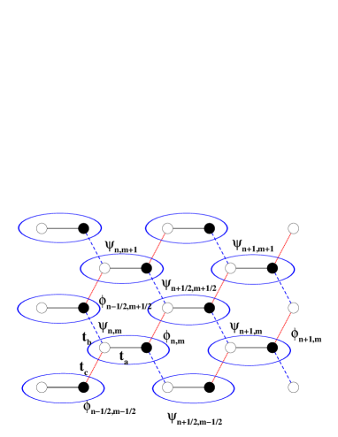
Figure 1: The honeycomb lattice. Open and closed circles shows sublattice A and B, respectively. $t_{a}$, $t_{b}$, and $t_{c}$ are hopping integrals.

The cylindrical geometry is taken and thus two edges are present. We consider three types of edges: zigzag, bearded, and armchair which are shown in Fig. 2.

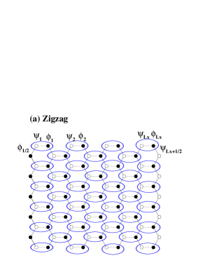
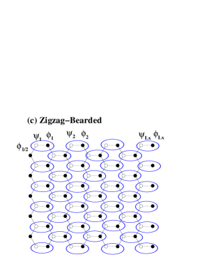
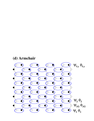
Figure 2: The honeycomb lattices with (a) zigzag ($L_{x}=4$), (b) bearded ($L_{x}=4$), (c) zigzag-bearded ($L_{x}=4$), and (d) armchair ($L_{y}=6$) edges, which we call Zigzag, Bearded, Zigzag-Bearded, and Armchair, respectively.

Two edges of the same type can form a cylinder. In addition, zigzag and bearded edges can form a cylinder. We call these as Zigzag, Bearded, Armchair, and Zigzag-Bearded, respectively. An armchair edge and a zigzag edge(or a bearded edge) can not form a pair of edges for a cylinder. When only nearest-neighbor hoppings are taken, the zero-energy edge states for Zigzag, Bearded, and Zigzag-Bearded are obtained. They are localized near the edges with the localization length

$$\xi=\frac{1}{2|\log t|},$$ (1)

where

$$t=\sqrt{2(1+\cos k_{y})}=2|\cos\frac{k_{y}}{2}|,$$ (2)

and $k_{y}$ is the reciprocal lattice vector in $y$-direction. We find the uniformly extended states at $|k_{y}|=\frac{2\pi}{3}$ as well as the strictly localized states at $|k_{y}|=\pi$. In addition, the origin of the states with macroscopic degeneracy at $|k_{y}|=\pi$ with $E=\pm 1$ are explained.

The localization length of Armchair diverges and there is no edge states if it is isotropic. We find edge states, however, if the system is anisotropic, i.e., three hoppings $t_{a}$, $t_{b}$, and $t_{c}$ are not equalhasegawaKonno ; hasegawaKohmoto .

Some of our results have been reported previously in the tight-binding modelklein ; fujita ; nakada ; wakabayashi1999 ; kusa ; hatsugai ; ezawa2006 ; peres2006 , the effective Dirac equationbrey2006 ; sasaki2006 ; abanin2006 and the first principle calculationsmiyamoto1999 ; okada2001 ; okada2003 ; lee2005 ; son2006 ; son2006b For the isotropic tight-binding model, Kleinklein has obtained the condition for the existence of the edge states for the bearded edge. Fujita et al.fujita obtained the conditions for the zigzag and armchair edges. However, there has been no studies of the anisotropic cases.

Due to the Dirac zero modes Jahn-Teller effect could take place in this system. Dynamical breaking of the lattice symmetry would give rise to anisotropy.

II Tight-binding model

Zigzag, Bearded, Zigzag-Bearded, and Armchair are shown in Figs. 2 (a), (b), (c), and (d). We pair a site on sublattice A and a site on sublattice B and denote the wave functions of a pair as $\psi_{n,m}$ and $\phi_{n,m}$ as shown in Fig. 1, where $n$ and $m$ are both integers or both half-integers. Then nearest neighbor hoppings give a tight-binding model

$$-t_{a}\psi_{n,m}-t_{b}\psi_{n+\frac{1}{2},m-\frac{1}{2}}-t_{c}\psi_{n+\frac{1}{2},m+\frac{1}{2}} =E\phi_{n,m}$$

$$-t_{a}\phi_{n,m}-t_{b}\phi_{n-\frac{1}{2},m+\frac{1}{2}}-t_{c}\phi_{n-\frac{1}{2},m-\frac{1}{2}} =E\psi_{n,m},$$ (3)

where $t_{a}$ is an intra-pair hoppings between $\psi_{n.m}$ and $\phi_{n,m}$, $t_{b}$ and $t_{c}$ and are inter-pair hoppings.

III Zigzag and Bearded

The zigzag edge and bearded edge can appear in the left edge or right edge. If the left edge is formed by the sublattice A or B, it is bearded or zigzag, respectively. If the right edge is formed by the sublattice A or B, it is zigzag or bearded, respectively.

We have edges in $y$-direction as shown in Figs. 2(a)-(c) and impose the periodic boundary condition, $\psi_{n,m+L_{y}}=\psi_{n,m}$ and $\phi_{n,m+L_{y}}=\phi_{n,m}$ in $y$-direction, where $L_{y}$ is an integer. Then one can write

$$\psi_{n,m}=\exp(ik_{y}m)\psi_{n}$$

$$\phi_{n,m}=\exp(ik_{y}m)\phi_{n},$$ (4)

where $k_{y}=\frac{2\pi j}{L_{y}}$ and $j=1,\ldots,L_{y}$ and (3) is written

$$\psi_{n}+t_{1}\psi_{n+\frac{1}{2}} = -\frac{E}{t_{a}}\phi_{n}$$

$$\phi_{n}+t_{2}\phi_{n-\frac{1}{2}} = -\frac{E}{t_{a}}\psi_{n},$$ (5)

where

$$t_{1}=\frac{t_{b}e^{-i\frac{k_{y}}{2}}+t_{c}e^{i\frac{k_{y}}{2}}}{t_{a}}$$ (6)

$$t_{2}=t_{1}^{*}=\frac{t_{b}e^{i\frac{k_{y}}{2}}+t_{c}e^{-i\frac{k_{y}}{2}}}{t_{a}}.$$ (7)

We define

$$t=|t_{1}|=|t_{2}|=\frac{\sqrt{t_{b}^{2}+t_{c}^{2}+2t_{b}t_{c}\cos k_{y}}}{t_{a}}.$$ (8)

When $t_{b}=t_{c}$, we have

$$t_{1}=\frac{2t_{b}}{t_{a}}\cos\frac{k_{y}}{2}.$$ (9)

III.1 Macroscopically degenerate states and the strictly localized states

If $t_{b}=t_{c}$ and $|k_{y}|=\pi$, $t_{1}$ and $t_{2}$ in (6) and (7) vanish and (5) becomes

$$\psi_{n} = -\frac{E}{t_{a}}\phi_{n}$$

$$\phi_{n} = -\frac{E}{t_{a}}\psi_{n}.$$ (10)

There is no inter-pair coupling and each pair is decoupled from others. This leads to macroscopic degeneracy. These are bulk states $E=\pm t_{a}$ for Zigzag, Bearded, and Zigzag-Bearded as shown in Figs 3, 7, and 8, respectively.

If we have $E=0$ in addition, pairs ($\psi_{n}$, $\phi_{n}$) vanish as seen from (10). Only non-vanishing wave functions are the unpaired ones at the edges. For Zigzag, the unpaired wave functions are $\phi_{1/2}$ and $\psi_{L_{x}+1/2}$. See Fig. 2(a). Thus we have strictly localized states $\phi_{1/2}$ at the left edge and $\psi_{L_{x}+1/2}$ at the right edge. (These states are extended in the $y$-direction.) For Bearded, there is no unpaired state as shown in Fig. 2(b), and there is no strictly localized state. For Zigzag-Bearded, $\phi_{1}$ is unpaired as shown in Fig. 2(c). This is the strictly localized state at the left edge. (This state is extended in the $y$-direction.)

III.2 Edge States

In the followings we implicitly assume the appropriate thermodynamic limit. If $E=0$, (5) is reduced to

$$\psi_{n} = -t_{1}\psi_{n+\frac{1}{2}}$$

$$\phi_{n} = -t_{2}\phi_{n-\frac{1}{2}}.$$ (11)

There is no intra pair coupling, namely $\psi_{n}$’s on sublattice A and $\phi_{n}$’s on sublattice B are decoupled.

III.2.1  Zigzag

As shown in Fig.2(a), the left edge has $\phi_{\frac{1}{2}}$ on sublattice B and the right edge has $\psi_{L_{x}+\frac{1}{2}}$ on sublattice A. The boundary condition on the left edge is to add a fictitious sites with $\psi_{\frac{1}{2}}=0$. In the same manner, the boundary condition on the right edge is to add a fictitious sites with $\phi_{L_{x}+\frac{1}{2}}=0$. Thus the boundary conditions for Zigzag are

$$\psi_{\frac{1}{2}} =0$$ (12)

$$\phi_{L_{x}+\frac{1}{2}} =0.$$ (13)

From (11) we obtain

$$\psi_{L_{x}-n} = (-t_{1})^{2n+\frac{1}{2}}\psi_{L_{x}+\frac{1}{2}}$$ (14)

$$\phi_{n} = (-t_{2})^{2n-1}\phi_{\frac{1}{2}}.$$ (15)

For the system with finite $L_{x}$, the solutions above are not exact. If $t<1$, however, (14) and (15) satisfy the boundary conditions in the limit $L_{x}\rightarrow\infty$ and these give the right edge states on sublattice A and the left edge states on sublattice B, respectively. Even if the system size is finite, we have the edge states with exponentially small $E$, when the edge states on the sublattices A and B coexist with negligibly small mixing to satisfy the boundary conditions.

The localization lengths for both sublattices are the same and given by

$$\xi=\frac{1}{2|\log{t}|}.$$ (16)

From (8), the condition for the existence of the edge states, $t<1$, is given by

$$\cos k_{y}<\frac{t_{a}^{2}-t_{b}^{2}-t_{c}^{2}}{2t_{b}t_{c}}.$$ (17)

Thus we have edge states for all the values of $k_{y}$ if $t_{b}+t_{c}<t_{a}$. There are no edge states if $|t_{b}-t_{c}|>t_{a}$.

For $t_{a}=t_{b}=t_{c}$, edge states exist if $|k_{y}|>\frac{2\pi}{3}$. The zero energy modes for these edge states are seen in Fig. 3.

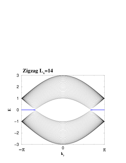
Figure 3: Energy spectrum for Zigzag for $L_{x}=14$. The zero energy modes for the edge states are on the blue lines.

An example of edge states are shown in Fig. 4

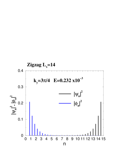
Figure 4: An example of the edge states.

III.2.2 Bearded

As shown in Fig. 2(b), the left edge has $\psi_{1}$ on sublattice A and the right edge has $\phi_{L_{x}}$ on sublattice B. The boundary conditions are given by

$$\psi_{L_{x}+\frac{1}{2}} =0$$

$$\phi_{\frac{1}{2}} =0.$$ (18)

In this case write (11) as

$$\psi_{n} = \left(-\frac{1}{t_{1}}\right)^{2n-2}\psi_{1}$$

$$\phi_{L_{x}-n} = \left(-\frac{1}{t_{2}}\right)^{2n}\phi_{L_{x}}.$$ (19)

If $t>1$, these are edge states with the localization length

$$\xi=\frac{1}{2\log{t}}.$$ (20)

For $t_{a}=t_{b}=t_{c}$, edge sates exist if $|k_{y}|<\frac{2\pi}{3}$. The energy spectrum in the isotropic case is plotted in Fig. 5.

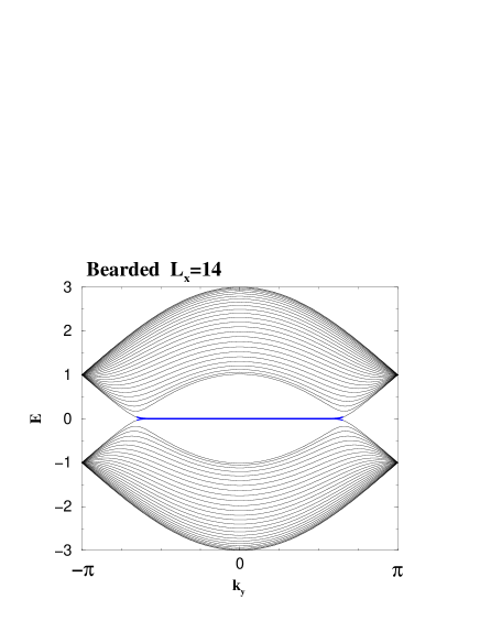
Figure 5: Energy spectrum for Bearded. The zero energy mode for the edge states are on the blue line.

III.2.3 Zigzag-Bearded

As shown in Fig. 2(c), the left edge is zigzag with $\phi_{\frac{1}{2}}$ on sublattice B. The right edge is bearded with $\phi_{L_{x}}$ also on sublattice B. The boundary conditions are given by

$$\psi_{\frac{1}{2}} =0$$ (21)

$$\psi_{L_{x}+\frac{1}{2}} =0.$$ (22)

These boundary conditions give $\psi_{n}=0$. Thus there are no edge states on sublattice A. There are no boundary condition for $\phi_{n}$. From (11) we have

$$\phi_{n} = (-t_{2})^{2n-1}\phi_{\frac{1}{2}}.$$ (23)

This is left edge states if $t<1$. On the other hand write

$$\phi_{L_{x}-n}=\left(-\frac{1}{t_{2}}\right)^{2n}\phi_{L_{x}},$$ (24)

then this gives right edge state if $t>1$.

The energy spectrum in the isotropic case, $t_{a}=t_{b}=t_{c}$, are shown in Fig. 6.

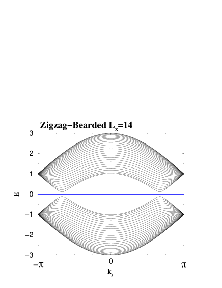
Figure 6: Energy spectrum for Zigzag-Bearded for $L_{x}=40$. The zero energy mode for the edge states are on the blue line.

The edge states are on the blue line which has the full length from $-\pi$ to $\pi$.

IV Armchair

We have the periodic boundary condition in $x$-direction, $\psi_{n+L_{x},m}=\psi_{n,m}$ and $\phi_{n+L_{x},m}=\phi_{n,m}$, as shown in Fig. 2(d). So write

$$\psi_{n,m} = \exp(ik_{x}n)\psi_{m}$$

$$\phi_{n,m} = \exp(ik_{x}n)\phi_{m},$$ (25)

where $k_{x}=\frac{2\pi j}{L_{x}}$ and $j=1,\ldots,L_{x}$. The boundary conditions at the edges are

$$\psi_{\frac{1}{2}} =\phi_{\frac{1}{2}}=0$$

$$\psi_{L_{y}+\frac{1}{2}} =\phi_{L_{y}+\frac{1}{2}}=0.$$ (26)

Let us consider the case where $E=0$ in which $\psi$’s and $\phi$’s are decoupled and satisfy

$$-t_{a}\psi_{m}-e^{i\frac{k_{x}}{2}}(t_{b}\psi_{m-\frac{1}{2}}+t_{c}\psi_{m+\frac{1}{2}}) = 0$$

$$-t_{a}\phi_{m}-e^{-i\frac{k_{x}}{2}}(t_{b}\phi_{m+\frac{1}{2}}+t_{c}\phi_{m-\frac{1}{2}}) = 0.$$ (27)

Put

$$\psi_{m}=z^{2m},$$ (28)

then from (27) we have two solutions for $z$ which satisfy

$$z_{\pm} = \frac{1}{2}\left[-\frac{t_{a}}{t_{c}}e^{-ik_{x}/2}\pm\sqrt{(\frac{t_{a}}{t_{c}})^{2}e^{-ik_{x}}-4\frac{t_{b}}{t_{c}}}\,\right]$$

$$z_{+}z_{-} = \frac{t_{b}}{t_{c}}$$

$$z_{+}+z_{-} = -\frac{t_{a}}{t_{c}}e^{-ik_{x}/2}.$$ (29)

In terms of these, the solution for (27) with the boundary condition $\psi_{\frac{1}{2}}=0$ is given by

$$\psi_{m}=\frac{z_{+}^{2m-1}-z_{-}^{2m-1}}{z_{+}-z_{-}}\psi_{1}.$$ (30)

This satisfies the boundary condition in the limit $L_{y}\rightarrow\infty$ if

$$|z_{+}|<1\;\mbox{and}\;|z_{-}|<1.$$ (31)

They are edge states localized near the bottom. In order (31) be satisfied,

$$t_{b}<t_{c}$$ (32)

is required as seen from (29).

In a similar manner, edge states localized near the top are possible if

$$|z_{+}|>1\;\mbox{and}\;|z_{-}|>1.$$ (33)

As seen from (29)

$$t_{b}>t_{c}$$ (34)

is required.

For analysis of $\phi$’s, we only need to replace $k_{x}$ by $-k_{x}$ and $t_{b}$ and $t_{c}$. This symmetry can be seen in Fig. (1) and also in Eq. (27). Thus we obtain essentially the same conditions.

See Figs. 7 and 8 for examples of the energy spectrum.

Figure 7: Energy spectrum for Armchair in the isotropic case. Neither (31) nor (33) are satisfied in this case. There is no edge state.

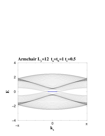
Figure 8: Energy spectrum for Armchair in an anisotropic case. The condition (33) is satisfied for certain $k_{x}$’s and edge states exist on the blue line.

V acknowledgement

We thank T. Aoyama for help with a computer calculation.

References

(1)
K. S. Novoselov, A. K. Geim, S. V. Morozov, D. Jiang, M. I. Katsnelson,
I. V. Grigorieva, S. V. Dubonos and A. A. Firsov,
Nature 438, 197 (2005)
(2)
Y. Zhang, Y.-W Tan, H. Stormer and P. Kim,
Nature 438, 201 (2005).
(3)
C. Berger, Z. Song, X. Li, X. Wu, N. Brown, C. Naud,
D. Mayou, T. Li, J. Hass, A.N. Marchenko, E. H. Conrad,
P. N. First, W. A. de Heer,
Science, 312, 1191 (2006).
(4)
Y. Hasegawa, R. Konno, H. Nakano and M. Kohmoto, Phys. Rev. B74, 033413 (2006).
(5)
Y. Hasegawa and M. Kohmoto,
Phys. Rev. B 74, 155415 (2006)
(6)
D.J. Klein, Chem. Phys. Lett. 217, 261 (1994)
(7)
M. Fujita, K. Wakabayashi, K. Nakada and K. Kusakabe,
J. Phys. Soc. Jpn. 65, 1920 (1996).
(8)
K. Nakada, M. Fujita, G. Dresselhaus and M. S. Dresselhaus,
Phys. Rev. B, 54, 17954 (1996).
(9)
K. Wakabayashi, M. Fujita, H. Ajiki, and M. Sigrist,
Phys. Rev. B 59, 8271 (1999).
(10)
K. Kusakabe and Y. Takagi,
Mol. Cryst. Liq. Cryst. 387, 7 (2002).
(11)
S. Ryu and Y. Hatsugai, Phys. Rev. Lett. 89, 077002 (2002).
(12)
M. Ezawa,
Phys. Rev. B 73 045432 (2006).
(13)
N. M. R. Peres, F. Guinea, and A. H. Castro Neto,
Phys. Rev. B 73, 125411 (2006).
(14)
L. Brey and H.A. Fertig,
Phys. Rev. B 73. 235411 (2006).
(15)
K. Sasaki, S. Murakami, and R. Saito,
J. Phys. Soc. Jpn., 75, 074713 (2006).
(16)
D. A. Abanin, P. A. Lee and L. S. Levitov,
Phys. Rev. Lett. 96, 176803 (2006).
(17)
Y. Miyamoto, K. Nakada, and M. Fujita, Phys. Rev. B. 59, 9858 (1999).
(18)
S. Okada and A. Oshiyama, Phys. Rev. Lett. 87, 146803 (2001).
(19)
S. Okada and A. Oshiyama,
J. Phys. Soc. Jpn. 72, 1510 (2003).
(20)
H. Lee, Y. W. Son, N. Park, S. Han, J. Yu,
Phys. Rev. B 72, 174431 (2005).
(21)
Y.W. Son, M.L. Cohen, and S. G. Louie, Phys. Rev. Lett. 97, 216803 (2006).
(22)
Y.W. Son, M.L. Cohen, and S. G. Louie, Nature. 444, 347 (2006).