Nearly-one-dimensional self-attractive Bose-Einstein condensates in optical lattices

Abstract

Within the framework of the mean-field description, we investigate atomic Bose-Einstein condensates (BECs), with attraction between atoms, under the action of strong transverse confinement and periodic (optical-lattice, OL) axial potential. Using a combination of the variational approximation (VA), one-dimensional (1D) nonpolynomial Schrödinger equation (NPSE), and direct numerical solutions of the underlying 3D Gross-Pitaevskii equation (GPE), we show that the ground state of the condensate is a soliton belonging to the semi-infinite bandgap of the periodic potential. The soliton may be confined to a single cell of the lattice, or extend to several cells, depending on the effective self-attraction strength, $g$ (which is proportional to the number of atoms bound in the soliton), and depth of the potential, $V_{0}$, the increase of $V_{0}$ leading to strong compression of the soliton. We demonstrate that the OL is an effective tool to control the soliton’s shape. It is found that, due to the 3D character of the underlying setting, the ground-state soliton collapses at a critical value of the strength, $g=g_{c}$, which gradually decreases with the increase of the depth of the periodic potential, $V_{0}$; under typical experimental conditions, the corresponding maximum number of ⁷Li atoms in the soliton, $N_{\max}$, ranges between $8,000$ and $4,000$. Examples of stable multi-peaked solitons are also found in the first finite bandgap of the lattice spectrum. The respective critical value $g_{c}$ again slowly decreases with the increase of $V_{0}$, corresponding to $N_{\max}\simeq 5,000$.

I Introduction

It has been firmly established in experiments with ultracold vapors of alkali metals that Bose-Einstein condensates (BECs) with weak attractive interactions between atoms (characterized by negative scattering length) can form stable matter-wave solitons in nearly one-dimensional (1D) “cigar-shaped” traps, which tightly confine the condensate in two transverse directions, but leave it almost free along the longitudinal axis. This setting has made it possible to create stable bright solitons Strecker02 ; Khaykovich02 and trains of such solitons Strecker02 in the ⁷Li condensate, where the interaction between atoms may be made weakly attractive by means of the Feshbach-resonance technique. In the ⁸⁵Rb condensate trapped under similar conditions, stronger attraction between atoms leads to the creation of nearly 3D solitons in a post-collapse state Cornish .

This experimentally relevant setting is described by effectively 1D equations which were derived, by means of various approximations, from the full 3D Gross-Pitaevskii equation (GPE) PerezGarcia98 -Napoli2 . In some cases, the deviation of the effective equation from the straightforward one-dimensional GPE with the cubic nonlinearity is adequately accounted for by an extra self-attractive quintic term, which may essentially affect the solitons Shlyap02 ; Brand06 ; Lev . The derivation of the 1D equation starts with adopting an ansatz factorizing the 3D wave function into the product of a transverse one (which amounts to the ground state of the 2D harmonic oscillator) and slowly varying axial (one-dimensional) wave function. The substitution of this ansatz in the variational approximation (VA; a review of the method can be found in Ref. Progress ) leads, without resorting to additional approximations, to a nonpolynomial Schrödinger equation (NPSE) for the longitudinal wave function sala1 ; sala2 . This equation was successfully used in various physical contexts sala3 ; sala4 . In particular, the above-mentioned simplified equation including cubic and quintic terms can then be obtained by an expansion of the NPSE for the case of a relatively weak nonlinearity Lev . A generalization of the NPSE for a two-component BEC was recently developed in Ref. we , in the form of a coupled system of NPSEs.

The objective of this work is to analyze the dynamics of quasi-1D solitons in the cigar-shaped trap equipped with a periodic potential, which can be easily created as an optical lattice (OL), by means of two coherent counterpropagating laser beams illuminating the condensate (for a recent review of the BEC dynamics in periodic potentials, see Ref. Markus ). Solitons in the 1D nonlinear Schrödinger equation (NLS) with the ordinary self-focusing cubic nonlinearity and periodic (lattice) potential had been studied some time ago 1Dtheory . It was shown that a stable soliton can be trapped by a local potential minimum of the OL. On the other hand, stable quasi-1D solitons in cigar-shaped traps exist up to a certain threshold, beyond which they suffer collapse. The occurrence of the collapse in the effective 1D equation reflects the presence of the collapse in the underlying 3D setting sala1 ; sala2 ; Lev . A new feature, which the present paper aims to report and explore, is the influence of the periodic potential on the collapse threshold for solitons in the quasi-1D trap. We demonstrate that, for both single-peak solitons found in the semi-infinite gap of the periodic potential, and multi-peaked solitons found in finite bandgaps, the collapse threshold gradually goes down with the increase of the potential strength. This feature may be explained by the fact that a sufficiently strong axial OL potential collects almost all the condensate in a limited space of a single lattice cell, thus facilitating the onset of the collapse. The predicted effect should be amenable to observation by means of standard experimental techniques.

The paper is organized as follows. In Section II, we apply the VA directly to the description of solitons in the underlying 3D GPE. In this way, the collapse threshold for the quasi-1D solitons is predicted in a semi-analytical form [in the same approximation, the stability of the solitons is estimated by means of the Vakhitov-Kolokolov (VK) criterion]. In Section III, we derive the one-dimensional NPSE in the presence of the periodic potential, and find soliton families as numerical solutions of the latter equation. Comparison with direct numerical solutions of the underlying 3D GPE demonstrates that the NPSE provides for very high accuracy in the prediction of both the shape of the solitons belonging to the semi-infinite gap and their collapse threshold; the accuracy provided by the VA is lower, but nevertheless reasonable too. In Section IV, we briefly consider examples of solitons belonging to the first finite bandgap. They are found in a numerical form from the corresponding NPSE. In the semi-infinite gap, the solitons may be narrow, occupying, essentially, a single site of the lattice potential, or broad, extending to several sites, but they always feature a single tall peak. The soliton in the finite bandgap has a very different shape, with many peaks. The paper is concluded by Section V.

II Variational approach

The energy-per-atom ($E$) and chemical potential ($\mu$) of the self-attractive BEC described by the mean-field stationary wave function, $\psi(\mathbf{r})$, in the presence of the strong transverse harmonic confinement with frequency $\omega_{\bot}$, acting in the plane of $\left(x,y\right)$, are

$$E=\int d\mathbf{r}\,\psi^{\ast}(\mathbf{r})\left[-{\frac{1}{2}}\nabla^{2}+{\frac{1}{2}}(x^{2}+y^{2})+U(z)-\pi g|\psi(\mathbf{r})|^{2}\right]\psi(\mathbf{r}),$$ (1)

$$\mu=E-\pi g\int\left|\psi(\mathbf{r})\right|^{4}d\mathbf{r.}$$ (2)

Here, the OL potential acting along axis $z$ is

$$U(z)=-V_{0}\cos{\left(2k_{L}z\right),}$$ (3)

with $k_{L}=\left(2\pi/\lambda\right)\sin\left(\theta/2\right)$, where $\lambda$ is the wavelength of two laser beams with angle $\theta$ between them that create the OL. We assume normalization $\int|\psi(\mathbf{r})|^{2}d\mathbf{r}\equiv 1$, then $g\equiv 2|a_{s}|N/a_{\bot}$ is the adimensional strength of the self-attraction, with negative scattering length of atomic collisions $a_{s}$, and the number of atoms in the condensate, $N$. Lengths in Eqs. (1) - (3) are measured in units of the transverse harmonic length, $a_{\bot}=\sqrt{\hbar/\left(m\omega_{\bot}\right)}$ ($m$ is the atomic mass), and the depth of the potential, $V_{0}$, is taken in units of $\hbar\omega_{\bot}$, therefore $\omega_{\perp}$ does not appear in the equations. For ⁷Li atoms in the transverse trap with $\omega_{\perp}=2\pi\times 1$ KHz, one has $a_{\bot}\simeq$ $1$ $\mu$m; then, $k_{L}=1$ (the value used in exampled displayed below) and $\lambda=1.5$ $\mu$m correspond to $\theta\simeq 30^{\circ}.$ In the same case, $V_{0}=1$ is tantamount, in physical units, to $\simeq 1.5E_{\mathrm{rec}}$, where the recoil energy for the OL with period $d\equiv\lambda/\left(2\sin(\theta/2\right))$ is $E_{\mathrm{rec}}=\left(\pi\hbar/d\right)^{2}/m$.

To predict solitons in an approximate analytical form, we use the 3D Gaussian ansatz,

$$\psi(\mathbf{r})={\frac{1}{\pi^{3/4}\sigma\eta^{1/2}}}\exp{\left\{-{\frac{(x^{2}+y^{2})}{2\sigma^{2}}-\frac{z^{2}}{2\eta^{2}}}\right\}},$$ (4)

where $\sigma$ and $\eta$ are, respectively, the transverse width and axial length of the localized pattern. Inserting this ansatz into Eqs. (1) and (2), we obtain

$$E={\frac{1}{2}}\left(\frac{1}{2\eta^{2}}+{\frac{1}{\sigma^{2}}}+\sigma^{2}\right)-{\frac{g}{2\sqrt{2\pi}}}{\frac{1}{\sigma^{2}\eta}}-V_{0}\exp{\left(-k_{L}^{2}\eta^{2}\right)},$$ (5)

$$\mu=E-{\frac{g}{2\sqrt{2\pi}}}{\frac{1}{\sigma^{2}\eta}.}$$ (6)

Aiming to predict the ground state in the framework of the above approximation, we look for values of $\sigma$ and $\eta$ that minimize energy $E$ [as given by Eq. (5)], using equations $\partial E/\partial\sigma=\partial E/\partial\eta=0$. This way, we derive coupled equations,

$$-{\frac{1}{\eta^{3}}}+{\frac{g}{(2\pi)^{1/2}}}{\frac{1}{\sigma^{2}\eta^{2}}}+4V_{0}k_{L}^{2}\eta\exp{\left(-k_{L}^{2}\eta^{2}\right)}=0,$$ (7)

$$-{\frac{1}{\sigma^{3}}}+\sigma+{\frac{g}{(2\pi)^{1/2}}}{\frac{1}{\sigma^{3}\eta}}=0,$$ (8)

which can be solved numerically method . Obviously, these solutions yield a ground state, i.e., a minimum of energy, only if the curvature of the energy dependence, $E(\eta,\sigma)$, is positive,

$${\frac{\partial^{2}E}{\partial\eta^{2}}}{\frac{\partial^{2}E}{\partial\sigma^{2}}}-\left({\frac{\partial^{2}E}{\partial\eta\partial\sigma}}\right)^{2}>0\;.$$

As concerns the dynamical stability of solitons against small perturbations, it may be, first of all, estimated by means of the VK criterion VK , according to which a necessary stability condition is $d\mu/dg<0$ (in the present notation), if the soliton family is described by dependence $\mu(g)$. Actually, the VK criterion may also be sufficient for the stability of solitons in the GPE with self-attraction and lattice  potential Salerno .

In Fig. 1, we plot solutions for $\sigma$ and $\eta$ of Eqs. (7) and (8), together with the corresponding energy-per-particle $E$ [calculated as per Eqs. (5)], as functions of interaction strength $g$, for several fixed values of potential depth $V_{0}$ and wavenumber $k_{L}=1$. Additionally, Fig. 2 displays respective dependences $\mu(g)$ of the soliton’s chemical potential, found from Eq. (6). The figures show that the soliton in the self-attractive BEC is predicted to exist up to a critical strength, $g_{c}$, which depends on $V_{0}$ and $k_{L}$. At $g>g_{c}$, the 3D collapse of the nearly-1D soliton occurs, as suggested by results obtained previously in models without the OL potential PerezGarcia98 ; sala1 ; sala2 . Note that the VA predicts $g_{c}=1.55$ for $V_{0}=0$ , which is somewhat higher than the critical value, $g_{c}=1.33$, obtained from a numerical solution of the full GPE with $V_{0}=0$ in three dimensions gammal ; sala2 . The characteristic value of the nonlinearity strength in Figs. 1 and 2, $g=1$, corresponds, for the above-mentioned transverse size, $a_{\perp}=1$ $\mu$m, and scattering length $a_{s}=-0.1$ nm, which can be attained in ⁷Li by means of the Feshbach resonance Strecker02 ; Khaykovich02 , to solitons built of $N\simeq 5,000$ atoms.

As $g$ drops to zero, the axial size of the soliton, $\eta$, diverges, while transverse width $\sigma$ approaches $1$ (in physical units, it becomes equal to the above-mentioned harmonic-oscillator length, $a_{\bot}$). On the other hand, as $g$ approaches $g_{c}$, both $\eta$ and $\sigma$ remain finite and smaller than $1$.

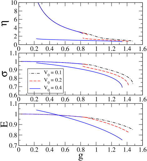
Figure 1: (Color online). Axial length $\eta$, transverse width $\sigma$, energy-per-particle $E$ of the quasi-1D soliton versus the self-attraction strength, $g\equiv 2|a_{s}|N/a_{\bot}$, as predicted by the variational approximation based on ansatz (4) and Eqs. (7), (8). The dependences are displayed at fixed values of depth $V_{0}$ of periodic potential (3), with $k_{L}=1$. On the right side, all curves terminate at a critical point, $g=g_{c}(V_{0})$, beyond which the collapse occurs (the upper curve in the top panel, which is cut by the panels’s frame, actually extends up to $g=0$, like its counterpart in the bottom panel.

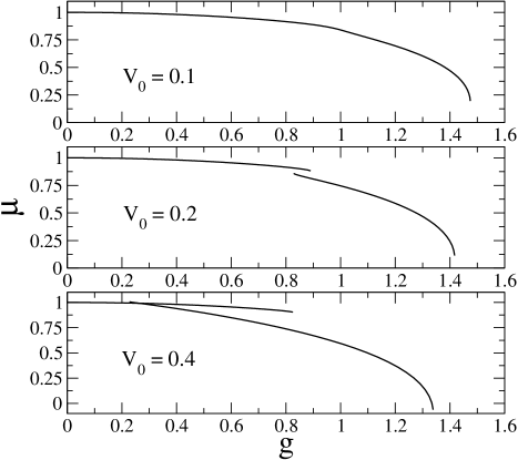
Figure 2: Continuation of Fig. 1: chemical potential $\mu$ of the quasi-1D soliton versus $g$, as predicted by the variational approximation for the same three values of $V_{0}$, and $k_{L}=1$.

At small $V_{0}$, the figure shows only a small distortion of the curves, and a small reduction of $g_{c}$, in comparison with the previously studied case of $V_{0}=0$. A qualitative change [which is best pronounced in Fig. 2, in terms of the $\mu(g)$ dependences] is observed at $V_{0}>0.15$ (i.e., for $\gtrsim 1,000$ atoms, according to the above estimate), when there appear two different stable branches. For $V=0.2$ and $V_{0}=0.4$, the lower branches of the $\eta(g)$ and $\sigma(g)$ dependences exists only in a finite interval, which we denote as

$$g_{m}<g<g_{c},$$ (9)

while the upper branches extend up to $g=0$, i.e., they exist in interval $0<g<g_{M}$, with $g_{M}<g_{c}$. Physically, the lower branches (with smaller values of axial length $\eta$) correspond to an attractive BEC which is localized, essentially, within a single cell of the OL; accordingly, we call the corresponding solution a single-site soliton. The upper branches of $\eta(g)$ and $\sigma(g)$ correspond to a weakly localized solution, which occupies several lattice sites; therefore, we call it a multi-site soliton. The bottom panel of Fig. 1 demonstrates that, for $V_{0}>0.15$, the multi-site soliton provides for smaller energy, i.e., it represents the ground state, at small $g$. At larger $g$, the single-site soliton becomes the ground state, while its multi-site counterpart is a metastable state. In particular, the above estimates demonstrate that, for $V_{0}=0.4$ (which is tantamount to $\simeq 0.6E_{\mathrm{rec}}$), the switch from the multi-site ground state to the single-site one occurs when the number of atoms (in the ⁷Li condensate) attains values $\sim 2,500$.

Figure 2 suggests that the families of soliton solutions are dynamically stable, as they always meet the VK criterion, $d\mu/dg<0$. In the case when two solutions exist, i.e., at $V_{0}>0.15$, both of them are VK-stable, i.e., the ground state and its metastable counterpart alike.

For $V_{0}>0.45$, the numeral solution of Eqs. (7) and (8) demonstrates that the lower threshold $g_{m}$ of existence interval (9) for the single-site soliton vanishes, but this is as an artifact of the VA, which is actually known in other contexts too Salerno . It is explained by inaccuracy of the Gaussian ansatz in the limit of weak nonlinearity, i.e., for widely spread small-amplitude solitons. In this situation, one may, in principle, apply a more sophisticated ansatz, combining the Gaussian and periodic functions, such as $\cos(2k_{L}z)$; however, the generalized ansatz results in a cumbersome algebra Arik , therefore we do not follow this way here.

It is interesting to predict the collapse critical strength, $g_{c}$, as a function of parameters $V_{0}$ and $k_{L}$ of the axial periodic potential. In Fig. 3, we display dependence $g_{c}(k_{L})$ predicted by the VA at four fixed values of $V_{0}$. For given strength $V_{0}$ of the potential, there exists wavenumber $k_{c}$ at which $g_{c}$ attains its minimum, i.e., the collapse has the lowest threshold. Further, Fig. 3 shows that this minimum of $g_{c}$ decreases with the increase of $V_{0}$, which may be understood as mentioned above: the strong potential tends to squeeze the entire condensate into a single call of the lattice, which facilitates the onset of collapse. On the other hand, at large values of $k_{L}$, $g_{c}$ is asymptotically constant, as the interaction of the condensate with the short-period OL becomes exponentially weak, see Eq. (5), hence it produces little effect on the collapse threshold.

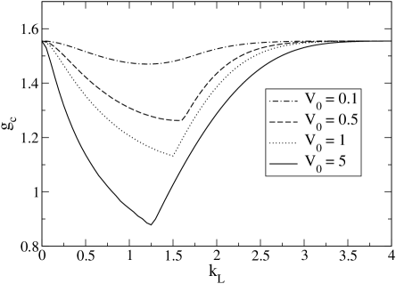
Figure 3: The critical value of the effective self-attraction strength, $g_{c}$, above which the soliton collapses, versus wave number $k_{L}$ of periodic potential (3). The results are obtained from the numerical solution of variational equations (7) and (8).

III Nonpolynomial Schrödinger equation

A more accurate analysis of the present setting may be performed using the one-dimensional nonpolynomial Schrödinger equation (NPSE) sala1 . As mentioned in Introduction, the derivation of the NPSE starts with the ansatz factorizing the 3D wave function into the product of the transverse 2D one, which describes the ground state of the harmonic oscillator, and a slowly varying 1D axial function, $f(z)$ (which may be complex),

$$\psi(\mathbf{r})={\frac{1}{\pi^{1/2}\sigma(z)}}\exp{\left\{-{\frac{(x^{2}+y^{2})}{2\sigma(z)^{2}}}\right\}}\,f(z).$$ (10)

Obviously, it is a more general ansatz than the above one, based on Eq. (4). Inserting expression (10) into Eq. (1), one finds [upon neglecting spatial derivatives of $\sigma(z)$] the following one-dimensional energy functional

$$E=\int dz\,f^{\ast}(z)\left[-{\frac{1}{2}}{\frac{d^{2}}{dz^{2}}}+{\frac{1}{2}}\left(\frac{1}{\sigma(z)^{2}}+\sigma(z)^{2}\right)\right.$$

$$\left.+U(z)-{\frac{1}{2}}\frac{g}{\sigma(z)^{2}}|f(z)|^{2}\right]f(z)\;.$$ (11)

Further, imposing an extra normalization condition,

$$\int_{-\infty}^{+\infty}dz\,|f(z)|^{2}=1,$$ (12)

on the 1D wave function and adding a term with the corresponding Lagrange multiplier, $\mu$ (which will again be the chemical potential), to energy functional (11), and, finally, minimizing the energy, one arrives at the following equations for real functions $f(z)$ and $\sigma(z)$ [where the expression (3) for the potential is substituted]:

$$\left[-{\frac{1}{2}}{\frac{\partial^{2}}{\partial z^{2}}}-V_{0}\cos{(2k_{L}z)}+\frac{1-(3/2)g|f(z)|^{2}}{\sqrt{1-g|f(z)|^{2}}}\right]f(z)=\mu f(z)\;,$$ (13)

$$\sigma(z)=\left(1-g|f(z)|^{2}\right)^{1/4}.$$ (14)

Equation (13) is the stationary version of the NPSE sala1 with the periodic potential, while $\mu$ is fixed by normalization condition (12). Note that only the 1D wave function, $f(z)$, appears in the NPSE, while the transverse width is locally expressed in terms of $f(z)$, as per Eq. (14). Equation (13) reduces to the familiar 1D cubic NLS equation for $gf^{2}\ll 1$ [then, Eq. (14) yields $\sigma\approx 1$]. Only in the latter case, the system may be considered as truly one-dimensional.

In previous studies which used the NPSE sala1 ; sala2 ; sala3 ; sala4 ; we , solitons were not considered in the presence of the periodic potential. In this work, we solved the full one-dimensional NPSE, which includes the time derivative and the periodic potential, numerically, using the finite-difference Crank-Nicholson method in imaginary time sala-numerics . In this way, we have obtained the soliton profiles shown in Fig. 4 for different values of the potential depth $V_{0}$ and fixed self-attraction strength, $g=0.5$ (recall it typically corresponds to $\sim 2,500$ atoms of ⁷Li bound in the soliton). As seen from the figure, the increase of the OL strength from zero to $\simeq 2$ recoil energies may compress the soliton, in the axial direction, by a factor $\gtrsim 4$. Generally, the use of the OL offers an efficient means to control the soliton shape (the OL may also be used as versatile tool to manipulate matter-wave solitons dynamically Panos ).

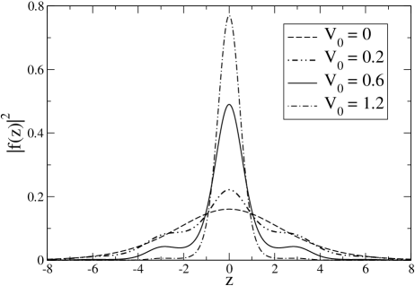
Figure 4: The axial density profile, $|f(z)|^{2}$, of the soliton in periodic potential (3), with $k_{L}=1$ and four different values of $V_{0}$. The self-attraction strength is fixed at $g=0.5$.

For $V_{0}=0$ (dashed line in Fig. 1), the shape of the soliton has a unique maximum, and the density profile may be well fitted to $f(z)=\left(\sqrt{{g}}{/2}\right)\mathrm{sech}\left(gz{/2}\right)$, which is rigorously valid in the above-mentioned limit corresponding to $gf^{2}\ll 1$, provided that $z$ varies in infinite limits. On the other hand, if $z$ belongs to  a finite interval, $-L/2<z<L/2$, with periodic boundary conditions, $f(z+L)=f(z)$, the NPSE with $V_{0}=0$ yields a spatially uniform profile of the ground state, $f(z)\equiv 1/\sqrt{L}$, for sufficiently weak nonlinearity, $0\leq g<\pi^{2}/L$; the ground state develops a spatial structure at $g>\pi^{2}/L$ ueda ; sala4 .

For nonzero but small $V_{0}$ (dot-dot-dashed and solid curves in Fig. 3), the soliton profile features several local maxima and minima due to the effect of the periodic potential notarella . Thus, under such conditions, the Bose condensate self-traps into a multi-peaked soliton, which occupies several cells of the periodic potential (the existence of stable three-dimensional multi-peaked solitons with a similar shape in the periodic axial potential, but without any transverse confinement, was demonstrated in Ref. Warsaw ; in that case, the transverse self-trapping and stability of the solitons was provided for by the “Feshbach-resonance-management” technique, i.e., periodic alternation of the sign of nonlinear coefficient $g$). Following the increase of $V_{0}$, the soliton compresses in the axial direction, and (for instance, at $V_{0}=1.2$, see the dot-dashed curve in Fig. 4) the secondary maxima become very small. In this case, the condensate actually self-traps into a single-peak soliton, which occupies only one cell of the OL (3).

Contrary to the sharp transition predicted by the VA in the previous section, the NPSE shows a smooth crossover from the multi-peak soliton to the single-peak one. In Fig. 5, we plot the axial length, $\sqrt{\left\langle z^{2}\right\rangle}$, of the ground-state bright soliton as a function of strength $g$, for $V_{0}=0.4$ (which is tantamount to the OL strength $\simeq 0.6$ recoil energy, as shown above), and compare the prediction of the VA with results produced by the NPSE. It is clearly seen that, while the VA predicts a jump at $g\simeq 0.5$, the NPSE does not show it. In fact, this jump is a consequence of the fact that ansatz (4), which assumes the simple Gaussian waveform for the axial wave function, provides for a crude fit to multi-peaked states. We also note that the numerical solution of the NPSE does not reveal the bistability predicted by the VA, as the numerical algorithm seeks for the ground-state solution for given $g$. For typical values of physical parameters mentioned above, Fig. 5 implies that, as the number of atoms increases from $1,000$ to $5,000$, the soliton shrinks in the longitudinal direction from $10$ to $1$ $\mu$m.

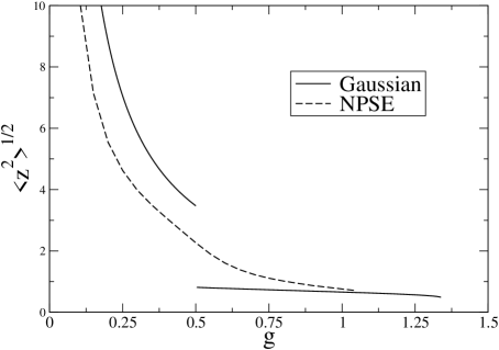
Figure 5: Axial length of the ground-state bright soliton, $\left\langle z^{2}\right\rangle^{1/2}$, as a function of self-attraction strength $g$, for $V_{0}=0.4$ and $k_{L}=1$ in Eq. (3). Displayed are results provided by the variational approximation based on the Gaussian ansatz, i.e., Eqs. (7) and (8), and by the nonpolynomial Schrödinger equation (NPSE), Eq. (13).

The VA developed in the previous section predicts the collapse of the soliton at the critical value of the self-attraction strength, $g=g_{c}$, which depends on parameters $V_{0}$ and $k_{L}$ of periodic potential (3). It is relevant to compare this prediction with results following from numerical solution of NPSE (13). In Table 1, we present the critical value, $g_{c}$, found from the NPSE for different values of $V_{0}$ and $k_{L}=1$. The results are in qualitative agreement with their variational counterparts displayed in Fig. 3: the increase of the potential depth, $V_{0}$, leads to gradual reduction of $g_{c}$. Note that the value of $g_{c}=1.33$ for $V_{0}=0$ is virtually the same as the above-mentioned numerically exact one, $g_{c}=1.34$, which was found from the numerical solution of the full three-dimensional GPE (with $V_{0}=0$) sala2 ; gammal . According to the above estimates, the drop of $g_{c}$ from $1.33$ to $0.85$ corresponds to the decrease of the maximum number of atoms from $N_{\max}\simeq 8,000$ to $N_{\max}\simeq 4,000$. For the sake of completeness, the table also shows the axial length and transverse width, obtained from Eqs. (13) and (14) at the collapse point, $g=g_{c}$. It is seen that the soliton shrinks in both directions with the increase of $V_{0}$, but its length and widths remain finite up to the collapse point. Typical values of the physical parameters referred to above imply that the data presented in Table 1 predict roughly constant density of the condensate at the collapse threshold, $\simeq 3\times 10^{14}$ cm^-3.

$V_{0}$	$g_{c}$	$\sqrt{\left\langle z^{2}\right\rangle}$	$\sigma(0)$
0	1.33	0.91	0.75
0.1	1.26	0.77	0.68
0.5	1.07	0.64	0.61
1	0.96	0.50	0.60
2	0.85	0.41	0.57

Table 1. The critical value of the self-attraction strength, $g_{c}$, and the corresponding values of the axial length, $\sqrt{\left\langle z^{2}\right\rangle}$, and minimal transverse width, $\sigma(0)$, of the soliton in the periodic potential, $V(z)=-V_{0}\cos\left(2k_{L}z\right)$, with $k_{L}=1$, for different values of $V_{0}$, as found from numerical solution of the 1D nonpolynomial Schrödinger equation, Eq. (13).

An important issue is the comparison of the results yielded by the NPSE with those found from direct numerical solution of the full 3D GPE in the presence of the axial periodic potential (in previous works dealing with the NPSE sala1 ; sala2 ; sala3 ; sala4 ; we , such a comparison was not presented for the model including the OL). It is also interesting to compare the results with those which can be obtained from the ordinary 1D cubic GPE [i.e., the 1D equation with the cubic nonlinearity and the same periodic potential, which can be obtained from Eq. (13) by expanding in small $g$ and keeping only terms up to the first order in $g$], since the latter equation is frequently used as a model of the BEC in the quasi-1D traps. Figure 6 shows that the density profiles generated by the NPSE are always very close to (practically, coincide with) the ones obtained from the 3D GPE. On the other hand, the profiles generated by the 1D cubic GPE are different, and the difference gets more pronounced with the increase of self-attraction strength $g$. This observation is not surprising because the nonlinearity in the NPSE essentially deviates from the cubic term if $g|f(z)|^{2}$ is large enough. Note also that the cubic GPE in one dimension cannot predict any collapse.

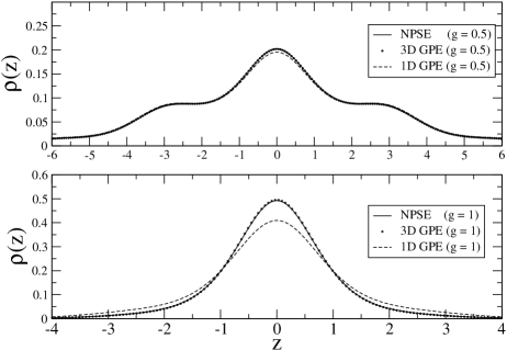
Figure 6: The axial density profile, $\rho(z)$, of the soliton in potential (3), with $k_{L}=1$ and $V_{0}=0.2$. Comparison between results provided by the different equations: NPSE, 3D GPE, and 1D GPE (the latter two with the cubic nonlinearity) is presented. In the case of the 3D equation, Eq. (1), the axial density is defined as $\rho(z)=\int\int|\psi(\mathbf{r})|^{2}dxdy$, while in the other cases it is simply $|f(z)|^{2}$.

IV Solitons in the finite bandgap

The above analysis was dealing with solitons whose chemical potential belongs to the semi-infinite bandgap in the linear spectrum of Eq. (13). On the other hand, it is known that the cubic self-attractive nonlinearity may also give rise to solitons located in higher-order (finite) bandgaps Canberra . This section addresses such solitons in the present model. It is relevant to stress that up to now, higher-bandgap solitons, in the case of self-attraction, have been considered only in strictly one-dimensional settings.

Here, we report soliton solutions found by means of the NPSE, Eq. (13), in the first finite bandgap corresponding to $k_{L}=1$. For this purpose, a self-consistent numerical method was used, with periodic boundary conditions. We employed a spatial grid of $1025$ points, covering the interval of $-50.26\leq z\leq 50.26$, which corresponds to $32$ periods of the external potential. To verify the correctness of the numerical scheme, we have checked that the lowest-energy state in the semi-infinite bandgap (i.e., the ground state of the system), produced by this method, is identical to that found above by the integration of the NPSE in imaginary time, i.e., the soliton shown in Fig. 4.

As a typical example, in Fig. 7 we plot the density profile, $|f(z)|^{2}$, of the 33th state (it is number 33 in the full set of the states generated by the numerical scheme) for $g=0.5$ and three different values of the potential depth, $V_{0}$. In the linear approximation, this state lies at the bottom of the second Bloch band. With the increase of nonlinearity strength $g$, the energy of the 33th state lowers, and, in doing so, it enters the first finite bandgap from above. At large values of $g$ (and small values of $V_{0}$), it passes the entire first bandgap from its top to the bottom, then crosses the band separating this bandgap from the semi-infinite gap, and eventually sinks into the latter one. Figure 7 shows that, for $V_{0}=0.2$, this state is still fully delocalized (being similar to a Bloch wave), while for $V_{0}=0.6$ it becomes localized, with a mean-square width much smaller than the length of the periodic box, featuring many local maxima and minima (zeros). We call this solution an excited multi-site soliton. Its multi-peaked structure is typical to gap solitons Canberra ; Markus ; BBB . At $V_{0}=1$, Fig. 7 shows that the excited soliton compresses itself into a narrower state. Simulations of the NPSE in real-time demonstrate that this soliton family is dynamically stable.

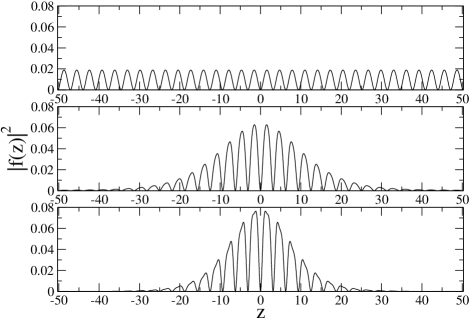
Figure 7: The axial-density profile, $|f(z)|^{2}$, of the lowest state in the first finite bandgap of periodic potential (3) with $k_{L}=1$. The self-attraction strength is $g=0.5$. The top, middle, and bottom panels correspond, respectively, to $V_{0}=0.2$, $V_{0}=0.6$, and $V_{0}=1$.

$V_{0}$	$g_{c}^{(1)}$	$\sqrt{\left\langle z^{2}\right\rangle}$
4	1.16	0.70
5	1.10	0.63
6	1.03	0.60
7	1.00	0.57

Table 2. The critical value of the self-attraction strength, $g_{c}^{(1)}$, of the lowest-energy state in the first finite bandgap of periodic potential (3), with $k_{L}=1$ and increasing values of its depth, $V_{0}$.  At $g>g_{c}^{(1)}$, collapse takes place. The soliton’s axial length, $\sqrt{\left\langle z^{2}\right\rangle}$, corresponding to to $g=g_{c}^{(1)}$, is tabulated too. Note that $\sigma(0)$ is always equal to $1$ because the soliton axial profile $|f(z)|^{2}$ has a node at $z=0$.

For the lowest-energy state in the first finite bandgap, there also exists a critical strength, $g_{c}^{(1)}$, of the self-attraction strength, above which the collapse occurs. In Table 2, we present these critical values corresponding to the increasing depth of the potential, $V_{0}$, which demonstrates gradual decrease of $g_{c}^{(1)}$. The latter dependence is qualitatively the same as reported above for solitons in the semi-infinite bandgap, cf. Table 1.

The axial size of the soliton at the collapse threshold ($g=g_{c}^{(1)}$) is also included in Table 1. As for the transverse width, $\sigma(z)$, in all cases it takes value $\sigma(0)=1$ at the center ($z=0$), unlike the solitons in the semi-infinite gap, cf. Table 1. This feature is explained by the fact that the amplitude of the gap soliton vanishes at $z=0$ (see Fig. 7), hence the width of the confined state at this point is the same as in the linear equation, i.e., $\sigma\equiv 1$ (according to the normalization adopted above).

In Table 2, we start with $V_{0}=4$ because for smaller $V_{0}$ the considered state plunges into the semi-infinite bandgap at $g$ close to $g_{c}^{(1)}$. According to the above estimates, the largest number of ⁷Li atoms possible in the soliton created in the first bandgap is $N_{\max}\sim 5,000$.

For the sake of completeness, in Fig. 8 we present the first $41$ eigenvalues $\epsilon_{j}$, as found from the stationary NPSE equation,

$$\left[-{\frac{1}{2}}{\frac{\partial^{2}}{\partial z^{2}}}-V_{0}\cos{(2kz)}+{\frac{1-{\frac{3}{2}}g|f_{j}(z)|^{2}}{\sqrt{1-g|f_{j}(z)|^{2}}}}\right]f_{j}(z)=\epsilon_{j}f_{j}(z)\,,$$ (15)

and plotted versus interaction strength $g$. The respective eigenfunctions, $f_{j}(z)$, may be both delocalized (Bloch-like) and localized (soliton-like). At $g=0$, the first $32$ eigenvalues generated by our numerical scheme belong to the first band, while the other nine fall into the second band. In compliance with the above discussion, Fig. 8 shows that the lowest eigenvalue and the 33th one split off from the first and second continuous bands and move down (up to the onset of the collapse) with the increase of $g$, thus giving rise to localized states, in the semi-infinite and first finite gaps, respectively. It is noteworthy that the second and third eigenvalues, which originally belong to the first band, also split off from it at larger values of $g$ (at largest values of $g$ displayed in Fig. 8, the fourth eigenvalues demonstrates the same trend). We have verified that the corresponding nonlinear eigenstates become localized, as one may expect. Note that similar results have been found in Ref. efremidis in a numerical solution of the ordinary cubic GPE in one dimension.

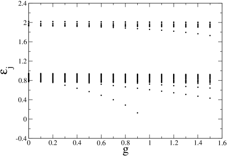
Figure 8: Eigenvalues $\epsilon_{j}$ found from Eq. (15) with $V_{0}=1$ and $k_{L}=1$, as functions of self-attraction strength $g$.

V Conclusions

In this work, we have considered soliton states in self-attractive BECs loaded into a cigar-shaped trap, which is equipped with a periodic OL (optical-lattice) axial potential. Using the 3D variational approximation (VA), and the effective NPSE (nonpolynomial Schrödinger equation) in one dimension, we have demonstrated that the ground state of the condensate is a bright soliton whose chemical potential falls within the semi-infinite bandgap created by the periodic potential. With the increase of the self-attraction strength, $g$, and/or the OL strength, $V_{0}$, the ground-state soliton changes its shape from broad (multi-site) to a narrow (single-site) one. In particular, the soliton composed of $\sim 2,500$ ⁷Li atoms trapped in the transverse harmonic potential with $\omega_{\perp}=2\pi\times 1$ KHz gets compressed by a factor of $4$, as $V_{0}$ increases from zero to two recoil energies; generally, the OL offers a convenient tool to control the shape of the soliton. The soliton solutions produced by the VA are stable against small perturbations, according to the VK (Vakhitov-Kolokolov criterion).

Due to the 3D nature of the trapped self-attractive condensate, the solitons exist up to a critical value, $g_{c}$, of $g$, beyond which the collapse takes place. A new feature reported in this work is the gradual decrease of $g_{c}$ with the increase of $V_{0}$, a qualitative explanation to which was given. For typical values of experimentally relevant parameters, the results translate into an estimate for the critical number of atoms at which the collapse occurs, which ranges from $8,000$ to $4,000$, while the critical density of the collapsing condensate is, roughly, constant, $\simeq 3\times 10^{14}$ cm^-3. Comparison with numerical solutions of the underlying 3D Gross-Pitaevskii equation shows that the NPSE very accurately predicts both the shape of the ground-state solitons and dependence $g_{c}(V_{0})$; the accuracy of the variational approximation is somewhat lower, but also reasonable.

Stable multi-peaked solitons were also found in the first finite bandgap of the OL potential. The respective critical nonlinearity strength again slowly decreases with the increase of $V_{0}$, the corresponding largest number of atoms in the soliton being estimated as $\sim 5,000$. It was studied in detail how the localized state splits off from the Bloch band and gives rise to the soliton in the first finite bandgap.

Finally,  it is relevant to mention that an interesting possibility, which deserves further consideration, is to induce an effective axial potential not directly, but rather through periodic modulation of the transverse tight-binding frequency Napoli . Another promising extension of the present analysis may be to the case of self-repulsive BEC loaded in the combination of the cigar-shaped trap and axial periodic potential. The study of the latter setting may shed new light on the theoretical description of quasi-1D gap solitons Markus ; Markus0 . These issues will be considered elsewhere.

References

- (1) K. E. Strecker, G. B. Partridge, A. G. Truscott and R. G. Hulet, Nature 417, 150 (2002); K. E. Strecker, G. B. Partridge, A. G. Truscott, and R. G. Hulet, New J. Phys. 5, 73 (2003).
- (2) L. Khaykovich, F. Schreck, G. Ferrari, T. Bourdel, J. Cubizolles, L. D. Carr, Y. Castin, and C. Salomon, Science 256, 1290 (2002).
- (3) S. L. Cornish, S. T. Thompson and C. E. Wieman, Phys. Rev. Lett. 96, 170401 (2006).
- (4) V. M. Pérez-García, H. Michinel, and H. Herrero, Phys. Rev. A 57, 3837 (1998).
- (5) L. Salasnich, Laser Phys. 12, 198 (2002); L. Salasnich, A. Parola, and L. Reatto, Phys. Rev. A 65, 043614 (2002).
- (6) L. Salasnich, A. Parola, and L. Reatto, Phys. Rev. A 66, 043603 (2002).
- (7) A. E. Muryshev, G. V. Shlyapnikov, W. Ertmer, K. Sengstock, and M. Lewenstein, Phys. Rev. Lett. 89, 110401 (2002).
- (8) S. Sinha, A. Y. Cherny, D. Kovrizhin, and J. Brand, Phys. Rev. Lett. 96, 030406 (2006).
- (9) L. Khaykovich and B. A. Malomed, Phys. Rev. A 74, 023607 (2006).
- (10) B. A. Malomed, in: Progress in Optics, vol. 43, p. 71 (E. Wolf, editor: North Holland, Amsterdam, 2002).
- (11) L. Salasnich, A. Parola, and L. Reatto, J. Phys. B: At. Mol. Opt. Phys. 39, 2839 (2006).
- (12) A. Parola, L. Salasnich, R. Rota, and L. Reatto, Phys. Rev. A 72, 063612 (2005); L. Salasnich, A. Parola, and L. Reatto Phys. Rev. A 74, 031603(R) (2006).
- (13) L. Salasnich and B. A. Malomed, Phys. Rev. A 74, 053610 (2006).
- (14) S. De Nicola, B. A. Malomed, and R. Fedele, Phys. Lett. A 360, 164 (2006).
- (15) S. De Nicola, R. Fedele, D. Jovanovic, B. Malomed, M. A. Man’ko, V. I. Man’ko, and P. K. Shukla, Eur. Phys. J. B 54, 113 (2006).
- (16) O. Morsch and M. Oberthaler, Rev. Mod. Phys. 78, 179 (2006).
- (17) B. A. Malomed, Z. H. Wang, P. L. Chu, and G. D. Peng, J. Opt. Soc. Am. B 16, 1197 (1999); G. Alfimov and V. V. Konotop, Physica D 146, 307 (2000).
- (18) Equations (7) and (8) are handled as a system of parametric equations, and , with parameter .
- (19) M. G. Vakhitov and A. A. Kolokolov, Radiophys. Quantum Electron. 16, 783 (1973).
- (20) B. B. Baizakov, B. A. Malomed, and M. Salerno, Europhys. Lett. 63, 642 (2003); Phys. Rev. A 70, 053613 (2004).
- (21) A. Gubeskys, B. A. Malomed, and I. M. Merhasin, Stud. Appl. Math. 115, 255 (2005).
- (22) E. Cerboneschi, R. Mannella, E. Arimondo, and L. Salasnich, Phys. Lett. A 249, 495 (1998); L. Salasnich, A. Parola, and L. Reatto, Phys. Rev. A 64, 023601 (2001).
- (23) P. G. Kevrekidis, D. J. Frantzeskakis, R. Carretero-Gonzalez, B. A. Malomed, G. Herring, and A. R. Bishop, Phys. Rev. A 71, 023614 (2005).
- (24) A. Gammal, L. Tomio, and T. Frederico, Phys. Rev. A 66, 043619 (2002).
- (25) R. Kanamoto, H. Saito, and M. Ueda, Phys. Rev. A 67, 013608 (2003); G.M. Kavoulakis, Phys. Rev. A 67, 011601(R) (2003).
- (26) In the system occupying a finite interval, , and with , the transition from the fully delocalized Bloch-wave ground state to a multi-site bright soliton can be estimated to occur at . This result is obtained by combining the multi-scale analysis [see, e.g., V. V. Konotop and M. Salerno, Phys. Rev. A 65, 021602(R) (2002)] with the perturbation theory (which assumes ) for the calculation of the effective mass and nonlinearity strength from the attractive cubic GPE in 1D, with the periodic potential.
- (27) M. Matuszewski, E. Infeld, B. A. Malomed, and M. Trippenbach, Phys. Rev. Lett. 95, 050403 (2005).
- (28) G. L. Alfimov, V. V. Konotop, and M. Salerno,Europhys. Lett. 58, 7 (2002); P. J. Y. Louis, E. A. Ostrovskaya, C. M. Savage, and Y. S. Kivshar, Phys. Rev. A 67, 013602 (2003).
- (29) B. B. Baizakov, V. V. Konotop, and M. Salerno, J. Phys. B: At. Mol. Phys. 35, 51015 (2002).
- (30) N. K. Efremidis and D. N. Christodoulides, Phys. Rev. A 67, 063608 (2003).
- (31) B. Eiermann, Th. Anker, M. Albiez, M. Taglieber, P. Treutlein, K.-P. Marzlin, and M. K. Oberthaler, Phys. Rev. Lett. 92, 230401 (2004).