Single Polymer Confinement in a Slit: Correlation between structure and dynamics

Abstract

In this paper, we construct an effective model for the dynamics of an excluded-volume chain under confinement, by extending the formalism of Rouse modes. We make specific predictions about the behavior of the modes for a single polymer confined to a slit. The results are tested against Monte Carlo simulations using the bond-fluctuation algorithm which uses a lattice representation of the polymer chain with excluded-volume effects.

I Introduction

Confining polymers inevitably leads to a competition between length scales arising from internal cooperativity and those imposed by external geometry, resulting in qualitative changes of the static and dynamic behavior. The effects of confinement on a single polymer chain is still not completely understood. A scaling picture has been used to describe the changes in the relaxational dynamics of a single, self-avoiding chain confined to a tube or a poreM. Daoud and J.P. Cotton (1982); F. Brochard and P.G. de Gennes (1977). Since a self-avoiding chain under cylindrical confinement models a variety of phenomena ranging from DNA translocation through synthetic poresA. Aksimentiev, J. B. Heng, G. Timp and K. Schulten (2004) to bacterial chromosome segregationP.J. Lewis (2001), there have been a number of simulation studies investigating its statics and dynamicsM. Daoud and J.P. Cotton (1982); K. Kremer, G.S. Grest, and I. Carmesin (1988); G. Morrison and D. Thirumalai (2005); R. M. Jendrejack, D. C. Schwartz, M. D. Graham and J.J. de Pablo (2003); K. Hagita and H. Takano (1998); A. Arnold and S. Jun (2007). In this paper, we use theory and simulations to study the dynamics of a single, self-avoiding polymer confined to a slit.

One of the key concepts in polymer dynamics is the relaxation of modes that describe the internal dynamics of a chain moleculeM. Doi (1995); F. Brochard and P.G. de Gennes (1977); A. Khoklov and A.I. Grosberg (1993). We construct a theoretical framework for describing the relaxation of the modes of a confined, self-avoiding chain in the absence of hydrodynamic interactions, by extending the Rouse modelM. Doi (1995). Our analysis shows that the anisotropy, introduced by the slit geometry, leads to dramatically different relaxations of the longitudinal and transverse modes. This effect, in turn, changes the nature of the motion of single monomers, and the collective dynamics of the self-avoiding chain. We perform simulations using the bond-fluctuation modelK. Kremer and I. Carmesin (1988), and show that the results can be explained, semi-quantitatively, by our theoretical model. Explicit theoretical results for the relaxation of Rouse modes, presented this work, provide a powerful tool for predicting fine scale and large scale motion of biopolymers within the confines of a cell.

II Rouse Modes

If excluded volume and hydrodynamic interactions are ignored, the dynamics of an unconfined, ideal chain (without self-avoidance) is well described by the Rouse modelM. Doi and S.F. Edwards (1988); M. Doi (1995):

$$\zeta\frac{\partial{\bf x}_{n}}{\partial t}=k({\bf x}_{n+1}-2{\bf x}_{n}+{\bf x}_{n-1})+{\bf g}_{n}{\bf(t)}$$ (1)

where ${{\bf x}_{n}}$ denotes the position of the $n^{th}$ monomer of size $b$, $k={k_{B}T\over{b^{2}}}$, ${\bf g}_{n}(t)$ is a random force arising from the solvent surrounding the polymer, and $\zeta$ is the friction constant of a single monomer. Considering dynamics at length scales much larger than the individual monomer size $b$,

$${\bf x}_{n+1}-2{\bf x}_{n}+{\bf x}_{n-1}\approx{\partial^{2}{\bf x}(n)\over\partial n^{2}}~{},$$ (2)

and Eq. (1) becomes a partial differential equation:

$$\zeta\frac{\partial{\bf x}(n,t)}{\partial t}=k\frac{\partial^{2}{\bf x}(n,t)}{\partial n^{2}}+{\bf g}(n,t)~{}.$$ (3)

The random force, ${\bf g}{(n,t)}$, is Gaussian and is characterized by the following correlations:

$$<{g}_{j}{(n,t)}>={\bf 0}$$ (4)

$$<{g}_{j}(n,t){g}_{k}{(n^{\prime},t^{\prime})}>={{{2k_{B}}T\zeta}\over{N}}\delta_{jk}\delta({t-t^{\prime}})\delta({n-n^{\prime}})$$ (5)

with $j$ and $k$ being the cartesian components of $\bf{g}(n,t)$, and $N$ the number of monomers in the chain. The normal modes of the above equation are the Rouse modes, and they decay exponentially with characteristic time scales that depend on the mode indexM. Doi and S.F. Edwards (1988); M. Doi (1995).

A major missing piece in the above description is excluded volume interactionsM. Doi and S.F. Edwards (1988). The inclusion of these interactions (or confinement) introduces couplings between the Rouse modes, and is described by an equation of the form:

$$\zeta\frac{\partial{\bf x}(n,t)}{\partial t}=k\frac{\partial^{2}{\bf x}(n,t)}{\partial n^{2}}+{\bf g}({\bf x},t)+{\bf F}(n,t)$$ (6)

where ${\bf F}(n,t)$ represents the force on the $n^{th}$ monomer due to all the other monomers, or due to the confining geometry. The presence of this term couples the Rouse modes, and in general, this equation has no analytic solution. An approach that has been used for unconfined, self-avoiding, polymers is to assume that the dynamics can still be described by decoupled Rouse modesM. Doi and S.F. Edwards (1988), but with renormalized parameters. Bond fluctuation algorithm simulations indicate that for such polymers, the Rouse modes are indeed weakly coupledK. Kremer and I. Carmesin (1988) and that the renormalized Rouse modes describe the dynamical behavior. The relaxation of the modes is characterized by a time scale $\tau_{p}\simeq{N^{2\nu}\over p^{2\nu+1}}$, where the mode index $p=0,1,2,.....$ , and $\nu$ is the Flory exponent: $\nu=3/(d+2)$ with $d$ being the spatial dimensionM. Doi (1995). In 2D, $\tau_{p}\simeq{N^{3/2}\over p^{5/2}}$. The longest relaxation time is $\tau_{1}\propto N^{2\nu+1}$, and is associated with the reorientation or rotation of the polymerM. Doi (1995).

II.1 Relaxation of Rouse Modes for Confined Polymers

In this work, we construct a framework for describing Rouse modes in confined polymers. To facilitate discussion, we briefly outline the steps leading to the results for unconfined polymers with self-avoidance. Neglecting the coupling between Rouse modes leads to a set of linear equations for the mode amplitudes $X_{pj}$M. Doi (1995); D. Molin, A. Barbieri, and D. Leporini (2006):

$$\zeta_{p}\frac{\partial X_{pj}}{\partial t}=-k_{pj}X_{pj}+g_{pj}{(t)}~{}.$$ (7)

Here

$$X_{pj}={1\over N}\int_{0}^{N}{dn\cos\left(p\pi n\over N\right)x_{nj}(t)}~{},$$ (8)

and $\zeta_{p}=2N\zeta$ for $p>0$, $\zeta_{0}=N\zeta$. All the self-avoidance and boundary effects are incorporated through the $k_{pj}$ term. Requiring that in the long time limit, the Rouse modes have the correct equilibrium distribution, implies thatM. Doi and S.F. Edwards (1988):

$$k_{pj}={k_{B}T\over<X_{pj}^{2}>_{eq}}$$ (9)

where $<.>_{eq}$ is an equilibrium average. The exact expression for $<X_{pj}^{2}>_{eq}$ can be derived using Eq.(8):

$$<X_{pj}^{2}>_{eq} = -{1\over 2N^{2}}\int_{0}^{N}\int_{0}^{N}dndm\cos\left({p\pi n\over N}\right)$$ (10)

$$\cos\left({p\pi m\over N}\right)\times<(x_{nj}-x_{mj})^{2}>$$

As shown by Doi and EdwardsM. Doi and S.F. Edwards (1988), for $p\gg 1$, $<X_{pj}^{2}>_{eq}$ can be expressed as:

$$<X_{pj}^{2}>_{eq} ={N\over{4p^{2}\pi^{2}}}\int_{0}^{N}{du}\cos\left(p\pi u\over N\right)\times$$ (11)

$$\frac{\partial^{2}<(x_{mj}-x_{nj})^{2}>_{eq}}{\partial n\partial m}$$

where $u=m-n$.

The generalized Rouse model treats a confined, self-avoiding polymer as an ideal polymer with renormalized spring constants. The utility of the approach relies on access to reliable results for the static correlations between monomers, $<(x_{mj}-x_{nj})^{2}>_{eq}$. The time scales associated with the relaxation of the Rouse modes, and ultimately the dynamics of the chain and single monomers can be obtained, once these static correlations are known. The task at hand is, therefore, to find an appropriate model for the equilibrium correlations for confined polymers and to predict the dynamical behavior using Eqs. (7)-(11)A. Arnold, B. Bozorgui, D. Frenkel, B. -Y. Ha and S. Jun (2007).

The next section is devoted to discussing appropriate forms for static correlations function of a confined, self-avoiding polymer.

III Blob Model for Slit Geometry

For an unconfined polymer, consisting of $N$ monomers of size $b$, represented as a self-avoiding-walk (SAW), the radius of gyration scales asP.J. Flory (1948):

$$R_{g} \sim bN^{\nu}$$

$${\nu} = {3\over{d+2}}$$ (12)

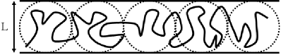
Figure 1: Sample configuration from simulation of a 2-D polymer confined to a tube. Circles indicate rough shape of the blobs and have a size on the order of the tube width, $L$.

Upon confining this SAW to a slit, we expect the excluded volume effects to change the monomer-monomer correlation functions. The scaling of these correlations with the tube width and length of the polymer has often been described by the blob modelF. Brochard and P.G. de Gennes (1977). Mean-field approaches have also been used to model these static correlationsG. Morrison and D. Thirumalai (2005); S.F. Edwards and P. Singh (1979).

In a slit of width $L$, the first effect of confinement is to make the polymer conformations anisotropicJ.H. van Vliet and G. ten Brinke (2005), and the shape needs to be characterized by a transverse ($R_{\perp}$) and a longitudinal ($R_{||}$) length scale. For widths, $L<R_{g}$, where $R_{g}$ is the radius of gyration of the unconfined polymer, confinement has the effect of stretching the polymer in the axial direction and screening out the excluded volume interactions beyond a length scale comparable to $L$. The polymer can be visualized as a succession of blobs with excluded-volume effects being maintained for distances smaller than the blob sizeF. Brochard and P.G. de Gennes (1977). The number of monomers per blob, $g$, can be calculated by requiring that the radius of gyration of these monomers matches the blob length scaleR. Azuma and H. Takayama (Jun 1999); T. Sakaue and E. Raphael (2006). For the slit geometry, the length scale of the blob is assumed to be $L$A. Arnold, B. Bozorgui, D. Frenkel, B. -Y. Ha and S. Jun (2007), and therefore,

$$g\sim\left({L\over b}\right)^{1/\nu}$$ (13)

The polymer is composed of $N_{b}=N/g$ blobs and has a lateral extension of:

$$R_{||}{=}LN_{b}=Nb(b/L)^{1/\nu-1}=Nb(b/L)^{1/3}~{},$$ (14)

where the last relation is specific for the slit geometry (2D). Since the tube width confines the polymer in the perpendicular directionP. Pincus (1976):

$$R_{\perp}{\propto}L$$ (15)

In papers by Edwards and Singh, estimates of polymer sizes were made using a mean-field approachS.F. Edwards and P. Singh (1979). This method was later applied to a polymer in a tube by Morrison and ThirumalaiG. Morrison and D. Thirumalai (2005). The blob predictions for the size of a polymer in narrow tubes agree with their estimates up to a factor of order unity.

III.1 Monomer-Monomer correlations in the Blob Model

The arguments presented above hold equally well for sub-chains as long as the sub-chains we consider are large enough to have the asymptotic behavior of a SAW. Therefore, the correlations between monomers in the directions parallel and perpendicular to the slit walls are should scale as:

$$<(x_{n||}-x_{m||})^{2}>\sim\left\{\begin{array}[]{ll}|n-m|^{3/2}b^{2}&\mbox{$|n-m|<\left(L\over b\right)^{4/3}$}\\ |n-m|^{2}b^{8/3}L^{-2/3}&\mbox{$|n-m|>\left(L\over b\right)^{4/3}$}\end{array}\right.\$$ (16)

$$<(x_{n\perp}-x_{m\perp})^{2}>\sim\left\{\begin{array}[]{ll}|n-m|^{3/2}b^{2}&\mbox{$|n-m|<\left(L\over b\right)^{4/3}$}\\ L^{2}&\mbox{$|n-m|>\left(L\over b\right)^{4/3}$}\end{array}\right.\$$ (17)

Recent simulationsA. Arnold, B. Bozorgui, D. Frenkel, B. -Y. Ha and S. Jun (2007) have measured the distribution of blob sizes by analyzing sub chains, and for strong confinement ($L<R_{g}$), their results are in agreement with the blob model predictions. In order to proceed with the dynamical calculations, we assume that the correlations are piecewise continuous with sharp transitions between the different scaling regimes represented in Eqs. (16) and (17).

III.2 Simulation results for the Monomer-Monomer correlation function

We have used simulations to measure the monomer correlations and compared them to the predictions of the blob model outlined above. To our knowledge, these predictions have never been directly confirmed.

Simulation Technique

Figure 2: Example chain configuration. Monomers occupy each box. Allowed moves are labeled with dashed arrows. Bonds are represented by solid lines.

The simulations were based on the bond fluctuation algorithm, a course-grained lattice-based algorithm that allows for the analysis of dynamical properties of polymersK. Kremer and I. Carmesin (1988). As the name implies, the algorithm allows for fluctuations of bond lengths and employs only local moves of monomers. Excluded-volume effects are taken into account by ensuring the initial polymer configuration contains no intersecting bonds and by allowing only the following set of bonds:

$$S = (2,0)\cup(2,1)\cup(2,2)\cup(3,0)\cup(3,1)\cup(3,2)$$

This also leads to an effective monomer size $b$, where $b\approx 2.8$ lattice spacings. This algorithm has been shown to reproduce the right scaling for polymer size and follow the generalized Rouse dynamics for excluded-volume polymersM. Doi (1995) in all spatial dimensions. It has been widely used to study the dynamics in different environmentsA. Di Cecca and J.J. Freire (2002); C.-M. Chen and Y.-A. Fwu (2000); N. Gilra, A.Z. Panagiotopoulos, and C. Cohen (2001); R. Azuma and H. Takayama (Jun 1999). In this paper, the simulation results are used to test the predictions of our theoretical formalism, and to explore in detail the dynamics of a chain confined to a slit.

Results

Monomer correlations were obtained for chains with $N=200$, $R_{g}=149$. This size is optimal in the sense that it is large enough to illustrate the effects of blobs while still yielding relaxation times that can be accommodated within accessible simulation times. As will be shown from our calculations of the Rouse mode relaxations, the longest time scale increases as $N^{3}$ and as $L^{-2/3}$, making it difficult to determine correlations functions for long chains in a narrow slit.

The initial chains were generated using a back-tracking algorithm which would redraw the part of the walk if a new segment had not been placed within $30$ attempts. To ensure little biasing from the generation of the initial walk, chains were equilibrated by allowing the chain to undergo $10^{8}$ monte carlo steps (mcs) ($200*10^{8}$ attempted moves). After equilibration, data was sampled every $10^{3}$ mcs for runs of $10^{8}$ mcs. The process was repeated for $10$ initial configurations and averaging was conducted over all sampled configurations of all runs as well as over the whole chain. This averaging leads to the data shown in Figs. 3 and 4.

The scaling laws observed in simulations are in broad agreement with the blob picture for the monomer correlations perpendicular to (Fig.3) and parallel to (Fig.4) the walls. In reporting the results of the simulations, we measure all lengths in units of $b$. Fig. 3 demonstrates that the data for the transverse correlations for different values of $L$ can be made to scale if $|n-m|$ is divided by $L^{4/3}$ and the correlations are scaled by $L^{2}$, confirming the form of Eq. 17, and the scaling of the blob size $g(L)$ as $L^{1/\nu}$ ($\nu=3/4$ in 2D). The results for the correlations in the longitudinal direction indicate a crossover between two power laws, as shown in Fig. 4.

According to the authors’ knowledge, this is the first direct test through simulations of distinct scaling regimes predicted by the blob model. Since there is broad support for the blob-scaling picture of monomer correlations from the simulations, we proceed to utilize these results for calculating the properties of the Rouse modes under confinement.

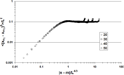
Figure 3: Scaling of $<(x_{n\perp}-x_{m\perp})^{2}>$ , demonstrating the the scaling of $g(L)$ as $L^{4/3}$, and validity of Eq. 17. The x-axis has been scaled by $L^{4/3}$, and th y-axis has been scaled by $L^{2}$. The chain length is $N=200$, $R_{g}=149$, and the slit widths are 20, 30, 40, and 50. All lengths are measured in units of the lattice spacing

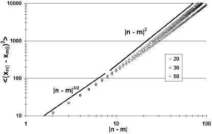
Figure 4: $<(x_{n||}-x_{m||})^{2}>$ versus slit width for the same set of parameters as Fig. 3. A crossover between two power laws is observed.

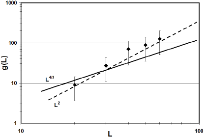
Figure 5: Scaling of the blob size, $g(L)$, extracted from the crossover points of $<(x_{n||}-x_{m||})^{2}>$ shown in Fig.4. The best fit is for $L^{2}$, however, the $L^{4/3}$ behavior evident in the transverse correlations is within the error bars on this data.

IV Relaxations of Rouse Modes

To study the dynamical correlations in the anisotropic geometry of the slit, we analyze the transverse modes, $X_{p\perp}$, and longitudinal modes , $X_{p||}$, separately.

Transverse Modes

The transverse modes correspond to taking $j$ to be in the direction perpendicular to the slit axis. The blob picture provides a natural scale of $p_{max}=N/g=Nb^{4/3}/L^{4/3}$, separating the large $p$ from the small $p$ regime. For $p<<p_{max}$, we use Eq.(17) directly in Eq.(10). For these modes, $<X_{p\perp}^{2}>_{eq}\simeq A-B(p/p_{max})^{2}$, where the constant $A={L^{10/3}\over{8\pi Nb^{4/3}}}$. In the regime where $L<<R_{g}$, modes with $p>p_{max}$, satisfy the condition for the use of Eq. (11), since these mode numbers satisfy $p>N(b/R_{g})^{4/3}=N$. Combining Eqs. (17) and (11) we, therefore obtain, for $p>p_{max}$,

$$<X_{p\perp}^{2}>_{eq}={N\over 4p^{2}\pi^{2}}\int_{0}^{(L/b)^{4/3}}{du}\cos\left(p\pi u\over N\right){b^{2}\over u^{1/2}}$$ (18)

$$<X_{p\perp}^{2}>_{eq}={N^{3/2}b^{2}\over 2^{3/2}p^{5/2}\pi^{2}}F_{c}\left(\sqrt{2p\over p_{max}}\right)$$ (19)

In the above equation, and below, we set $b=1$, and $\zeta/{k_{B}T}=1$. The relaxation of the transverse modes is exponential with a time scale:

$$\tau_{p\perp}={\zeta_{p}\over k_{p\perp}}=N<X_{p\perp}^{2}>_{eq}$$ (20)

A reasonable approximation of $F_{c}(x)$, the Fresnel Cosine function, is a linear function of the argument for $x\ll 1$ and $1/2$ for $x\gg 1$. For $p>p_{max}$,the argument of $F_{c}(x)$ is always greater than $1$, and, therefore, $\tau_{p\perp}$ scales as $1/p^{5/2}$, which is a form identical to the relaxation of unconfined modes. This result provides a self-consistency check on our calculations, since the blob model assumes that the correlations within the blob are identical to that of an unconfined chain.

These results show that $<X_{p\perp}^{2}>_{eq}$ decreases monotonically with $p$, initially as $A-Bp^{2}$, and then as $p^{5/2}$. The slowest transverse mode is, therefore, $p=1$, and the associated relaxation time is given by :

$$\tau^{\perp}\propto L^{10/3}/(8\pi)$$ (21)

Longitudinal Modes

For modes with $p>p_{max}$, the functional form of the mode amplitudes is the same as that for the transverse modes:

$$<X_{p||}^{2}>_{eq}={N^{3/2}b^{2}\over 2^{3/2}p^{5/2}\pi^{2}}F_{c}\left(\sqrt{2p\over p_{max}}\right)$$ (22)

For $p<p_{max}$, we use Eq.(16) directly in Eq.(10). In the limit of small slit widths, $L\ll Nb$, we obtain a closed form expressionY.-J. Sheng and M.-C. Wang (2001):

$$<X_{p||}^{2}>_{eq}\sim{(1-(-1)^{p})N^{2}\over p^{4}L^{2/3}}+(O){L^{2/3}}$$ (23)

In the small $p$ regime, therefore, the odd and even modes behave differently. The odd modes exhibit a $p^{4}$ decay of $<X_{p||}^{2}>_{eq}$, and dominate for small $L$, since the leading term in Eq. 23 vanishes for the even modes. For $p>N/g$, Eq. 22 implies that $<X_{p||}^{2}>_{eq}$ decays as $p^{5/2}$

The longest relaxation time in the longitudinal direction is determine by the relaxation of the $p=1$ mode. and is given by:

$$\tau^{||}=2N^{3}/L^{2/3}$$ (24)

Unlike $\tau^{\perp}$, this time-scale increases as the slit width $L$ decreases. The equilibration time is dominated by the relaxation of the $p=1$, longitudinal mode, and as we will show from the simulations, corresponds to a collective rearrangement of the chain where the end-to-end vector changes sign.

In the next sections, we will use the results for the Rouse modes to analyze the dynamical properties of the confined chain.

IV.1 Collective Dynamics

The longest relaxation time of an unconfined polymer chain is associated with the relaxation of the end-to-end vector, $\bf P(t)=\bf R_{N}(t)-\bf R_{0}(t)$ and is reflected in the autocorrelation function:

$$C(t)=\langle\bf P(t)\cdot\bf P(0)\rangle$$ (25)

The Rouse model result for an unconfined, self avoiding polymer isM. Doi (1995):

$$C(t)\sim\exp\left(-{t\over\tau_{1}}\right)$$ (26)

where $\tau_{1}$ is the relaxation time of the $p=1$, unconfined Rouse mode: $\tau_{1}\sim N^{3/2}$ in 2DM. Doi (1995).

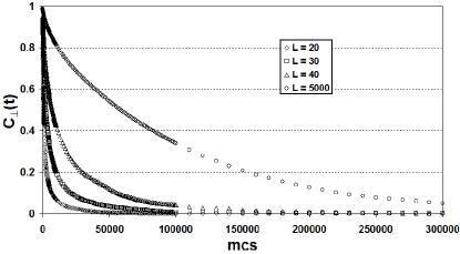
Figure 6: Simulation Results: End-to-end correlation function in the perpendicular direction for a chain 50 monomers long and for slit widths of 20, 30, 40, and 5000 lattice spaces.

In a slit, we need to look at the relaxation of the perpendicular and parallel components of $\bf P(t)$, separately. Writing $C_{\perp}(t)$ and $C_{||}(t))$ in terms of the Rouse modesM. Doi (1995), it becomes evident that the long-time relaxation is exponential with a time scale given by the longest-lived transverse and longitudinal modes, respectively. From the analysis of Rouse modes for the confined polymers, it follows, therefore, that

$$C_{\perp}(t) \sim \exp\left(-{t\over\tau^{\perp}}\right)=\exp\left(-2^{1/2}\pi^{2}t\over L^{10/3}\right)$$

$$C_{||}(t) \sim \exp\left(-{t\over\tau^{||}}\right)=\exp\left(-tL^{2/3}\over 2N^{3}\right)$$ (27)

These results demonstrate that the collective dynamics of a polymer confined to a slit is qualitatively different from an unconfined polymer. The relaxation time of the longitudinal component of the end-to-end vector increases dramatically as $L$ is decreased, diverging as $L\rightarrow 0$. This increase in relaxation time has been observed in earlier simulationsA. Arnold, B. Bozorgui, D. Frenkel, B. -Y. Ha and S. Jun (2007) and, as shown in Figs. 7 and 8 is captured by our simulations.

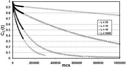
Figure 7: Simulation Results: End-to-end correlation function for component parallel to the walls for a chain with $N=50$, $R_{g}=53$, and for slit widths of 20, 30, 40, and 5000 (unconfined).

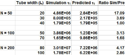
Figure 8: Simulation Results: Observed value of longest odd mode versus predicted value. A factor of 16.75 is chosen as to match up the time scales at one point $(N=50,L=40)$. This factor absorbs any dependence on the monomer size $b$. The slit width is in units of lattice spacing.

Since the time scale associated with changes in orientation of the end-to-end vector increases as $N^{2}L^{-2/3}$, long Monte Carlo runs are required to ensure that chain configurations and their mirror images are sampled equally. In order to keep the simulations manageable, we studied relatively short chains, $N=50$ monomers long. The results were averaged over $10^{9}$ mcs after initial equilibration of $10^{8}$ mcs steps and for $5$ different initial configurations.

In the unconfined polymer, the slowest mode corresponds to the reorientation of the end-to-end vector and the time scale increases as $R_{g}^{2}$. Under confinement, the slowest mode still involves reorientation, but now the time scale is expected to go as $R_{||}^{2}\sim N^{2}L^{-2/3}$, as obtained from our analysis of the Rouse modes. Based on these arguments, the reorientation events are expected to become increasingly rare as $L$ is decreased. This expectation is borne out in our simulations, as evidenced by the time traces in Fig.9.

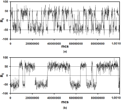
Figure 9: Simulation Results: Time trace of the longitudinal component of the end-to-end vector $\bf P(t)$ for a chain with $N=50$, $R_{g}=53$, and for slit widths of (a) 40 and (b) 30.

One way of describing fluctuations of the confined polymer is to say that the chain fluctuates about a fixed shape, characterized by the direction of ${\bf P}(t)$, changing shape only occasionally. The fluctuations about the shape are described by the transverse Rouse modes, which as Eq.21 shows, relax faster as the slit width is decreased, and are independent of the size of the chain. Results from our simulations shown in Fig. 6 are consistent with these predictions. In simulations of a model polymer confined in a 2D boxA. Rahmanisisan, C. Castelnovo, J. Schmit, and C. Chamon (2007), it has been observed that the slow modes correspond to shape changes, and that the slow dynamics is not reflected directly in the monomer motion. The shape of the polymer is a simpler variable in the slit geometry, but a distinct separation between time scales associated with shape changes and time scales associated with individual monomer motion is predicted by the generalized Rouse dynamics, and seen in the simulations.

In the next section, we analyze the motion of monomers using the framework of the Rouse modes.

IV.2 Monomer Motion

In this section, the effective Rouse modes are used to make detailed predictions for the mean-squared-displacement (MSD) of monomers. The theory for the MSD of monomers should provide a framework for understanding the dynamics inside biological cells where motion has been observed to be subdiffusiveA. Fiebig, K. Keren and J. A. Theriot (2006).

Starting from Eq.(8) and making use of the fact the perpendicular mode index has a lower bound of $N/g$, the number of blobs, it can be shown that the displacement squared of a monomer in the direction perpendicular to the walls is

$$<(x_{n\perp}(t)-x_{n\perp}(0))^{2}>=\sum_{p=(N/g)}^{\infty}{4\over k_{p\perp}}\left[1-exp\left(-{t\over\tau_{p\perp}}\right)\right]$$ (28)

Likewise the expression for the parallel monomer motion is

$$<(x_{n||}(t)-x_{n||}(0))^{2}>={2t\over N}+\sum_{p=1}^{\infty}{4\over k_{p||}}\left[1-exp\left(-{t\over\tau_{p||}}\right)\right]$$ (29)

Figure 10: Prediction for perpendicular motion from theory for a chain of 200 monomers, monomer size 2.8, and slit width 30 ($L/R_{g}=1/5$). (see Eq.(28))

The main features of the perpendicular motion, as predicted by (28), are depicted in Fig.(10). Since $k_{p\perp}$ has the same functional form as the unconfined polymer modes for $p\geq N/g$, the MSD exhibits a $t^{3/5}$ power law that saturates to a value proportional to $L^{2}$ for $t\gg\tau^{\perp}$, the relaxation time of the $p=N/g$ mode. The explicit exponent of $3/5$ can be obtained by analyzing Eq. 28 for $t\ll\tau^{\perp}$. In this limit, the sums can be replaced by integrals, and we obtain:

$$<(x_{n\perp}(t)-x_{n\perp}(0))^{2}>\approx{2^{16/5}b^{4/3}\over 3\pi^{4/5}}t^{3/5}\Gamma_{q}(2/5)~{}.$$ (30)

In the above equation, $\Gamma_{q}$ is the Gamma function, and $q={b^{4/3}\pi^{2}t\over 2^{1/2}L^{10/3}}$. The results of simulations for a $N=200$ chain confined to slit widths ranging from $20$ to $50$ are shown in Fig. 11. As predicted by the theory, MSD for different values of $L$ can be collapsed on to each other by scaling the time $t$ by $\tau^{\perp}\sim L^{10/3}$ and scaling the MSD by its maximum value which increases as $L^{2}$ (Fig. 12).

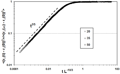
Figure 11: Simulation Results: Plots of MSD of the perpendicular component of the middle monomer in a chain with $N=200$ The MSD have been rescaled by the maximum value of the saturation value at each $L$, and time has been scaled by, $L^{-10/3}$, to capture the scaling of $\tau^{\perp}$. These scalings lead to data collapse for $L=20~{},35~{},{}50$.

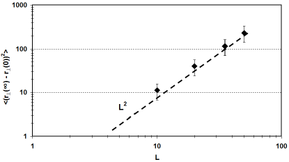
Figure 12: Simulation Results: Plots of saturation value of displacement squared of the perpendicular component of the middle monomer in the chain recovered from simulations. The chain is 200 monomers long and plots are for slit widths of 10, 20, 35, 50.

The MSD in the longitudinal direction, described by Eq. 29, is expected to exhibit multiple regimes. The functional form of of the effective spring constants, $k_{p||}$, changes at $p=N/g$ with a $p^{4}$ increase at low $p$ (for the odd modes) and a $p^{5/2}$ increase for the high $p$ modes. The analysis is further complicated by the difference between odd and even modes for low mode numbers.

Figure 13: Results for the MSD in the longitudinal direction obtained by numerical evaluation of Eq.(29) for a chain of 200 monomers, monomer size 2.8, and slit width 30. The dashed lines and the arrows mark the power laws and the crossover times predicted by the short-time approximation, Eq. (IV.2)

Even though there is no closed form expression for the MSD in the longitudinal direction, we can recover useful information about the functional forms and crossover times. To accomplish this, we look at times much less than the longest relaxation time of the system. With this assumption, the sum in (29) can be approximated as an integral and results in the following closed form expressionsJ. Kalb (2008):

$$<(x_{n||}(t)-x_{n||}(0))^{2}>\approx{2t\over N}+$$

$${2^{16/5}b^{4/3}\over 3\pi^{4/5}}t^{3/5}\Gamma_{b^{4/3}\pi^{2}t\over 2^{1/2}L^{10/3}}(2/5)+$$ (31)

$${2^{7/2}b^{2/3}L^{1/3}\over\pi^{1/2}}t^{1/2}Erf\left({\pi b^{2/3}t^{1/2}\over 2^{1/2}L^{5/3}}\right)$$

where we have made explicit use of Eq. (22). As expected, the ${0}^{th}$ mode leads to purely diffusive motion. The system is dominated by the $t^{3/5}$ behavior until a crossover time of associated with relaxations within the blob, $\tau_{B||}$:

$$\tau_{B||}={2L^{10/3}\over\pi^{2}b^{4/3}}~{},$$ (32)

which is proportional to $\tau^{\perp}$. For times longer than $\tau_{B||}$, $t^{1/2}$ is the dominant behavior, and this subdiffusive motion becomes diffusive as the $0{th}$ mode starts dominating at $\tau_{D||}$P.G. de Gennes (1971):

$$\tau_{D||}={8b^{4/3}N^{2}L^{2/3}\over\pi}$$ (33)

These time scales, and the power laws are shown in Fig.13.

The different power-law regimes correspond to physically different relaxation mechanisms. At the shortest time scales, the relaxation is not affected by the confinement, and the MSD follows that of the unconfined, self-avoiding chain. At intermediate times, the polymers can be thought of as an ideal chain of blobs, and blob compression dominates the dynamicsF. Brochard and P.G. de Gennes (1977). The MSD, therefore, shows the sub-diffusive behavior characteristic of an ideal chain with no excluded volume constraint. The long-time diffusive motion reflects the center-of-mass motion. An interesting observation to be made is that the diffusive behavior sets in at earlier and earlier times as the slit width $L$ is decreased. This apparently counterintuitive result, however, follows from the fact that with increasing confinement, transverse fluctuations decay faster, ($\tau^{\perp}\sim L^{10/3}$), and the longitudinal motion of the polymer essentially looks like that of a rigid rod. The reorientation events, which are the slowest dynamical process in the system, do not affect the MSD of monomers.

The above analysis relies on our deductions for the functional form of the amplitudes $\langle X_{p||}^{2}\rangle$, which determine $k_{p||}$. We have extracted the Rouse mode amplitudes from the simulations (see Fig.14) to directly verify these functional forms. We find that for mode numbers $p$ greater than a characteristic value $p_{s}$, the amplitudes decay as $p^{-5/2}$, just as they do in the unconfined chain. However, for $p\leq p_{s}$, there is an observed splitting in the even and odd modes, with the even modes seemingly exhibiting a $p^{-2}$ behavior and the odd modes decaying as $p^{-4}$. Since we can obtain data only over a limited range (determined by the size of the chain), these power laws are only approximate. The crossover at $p_{s}$ is a robust phenomenon. From our theoretical analysis, we expect $p_{s}=N/g$. For a chain of $N=200$, $b=2.8$ (characteristic of the bond-fluctuation model), and a slit width of $L=30$, the blob model predicts that $N/g=8.0$. The simulation data (Fig.14)) is in surprisingly good agreement with this prediction. Our simulation results, therefore, support the conclusion that the statistical properties of the confined polymer can be understood in terms of the effective Rouse modes obtained from our theoretical framework.

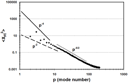
Figure 14: Simulation Results: Mode excitation vs mode number $p$ extracted from simulation for a chain 200 monomers long and a slit width of 30 lattice space. The saturation value for the largest modes is due to the chain being discrete instead of continuous. Solid and dashed lines represent the linearized Rouse theory predictions.

We have used our simulations to carefully measure the MSD of monomers in the longitudinal direction, and the results are shown in Figs. 15 and 16. Our results are consistent with the theoretical predictions. The short time behavior is governed by a sub-diffusive, $t^{3/5}$ regime, associated with the unconfined polymer. There is a hint of an intermediate regime, governed by the slower power law of $t^{1/2}$. Finally, at long times, the MSD is observed to increase linearly with $t$. The two characteristic times associated with the crossover from $t^{3/5}$ to $t^{1/2}$ ($\tau_{B||}$) and $t^{1/2}$ to $t$ ($\tau_{D||}$) are plotted in Fig.16 and both times are observed to be monotonically decreasing with the tube widths, approximately obeying the scaling predicted by Eqs. (32) and (33).

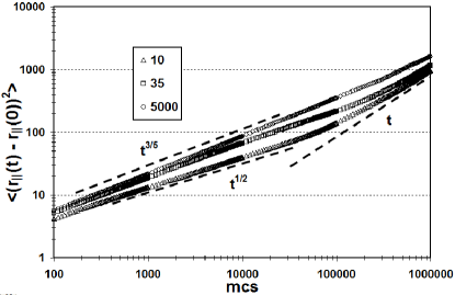
Figure 15: Simulation Results: MSD of the middle monomer parallel to the slit walls for a chain of length 200 and the slit widths shown in the figure. For the unconfined chain, $L=5000$, the diffusive regime is barely visible at $t=10^{6}$ mcs. In contrast, for $L=10$, the diffusive regime is visible at $t=10^{5}$ mcs.

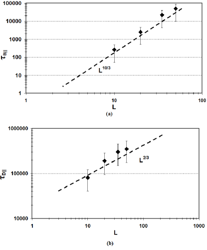
Figure 16: Simulation Results: $\bf{(a)}$ Plot of first crossover time from $t^{3/5}$ to $t^{1/2}$ ($\tau_{B||}$) from Fig.15.$\bf{(b)}$ Plot of first crossover time from $t^{1/2}$ to $t$ ($\tau_{D||}$) from Fig.15.

V Conclusion

We have presented a theoretical framework for analyzing the dynamics of confined, self-avoiding polymers that is valid for any confining geometry. The formalism is based on renormalized, effective, Rouse modes. Through extensive simulations, we have shown that he predictions of the theory are borne out for a polymer chain confined to a slit.

Given the Rouse mode framework, both collective dynamics and single monomer motion can be determined from a knowledge of the mode relaxations. Our analysis shows that confinement introduces multiple time scales into the dynamics. The slowest mode is associated with the reorientation of the end-to-end vector, and its relaxation time increases as $L^{-2/3}$ with decreasing slit width. Transverse fluctuations of the chain relax on a time scale that decreases as $L^{10/3}$. This latter time scale shows up in the monomer dynamics as a crossover time from a $t^{3/5}$ subdiffusive behavior, characteristic of the self-avoiding polymer, to a $t^{1/2}$ subdiffusive behavior, characteristic of an ideal, phantom chain. In an unconfined polymer this intermediate regime is absent. Under confinement, the monomers exhibit pure diffusion in the longitudinal direction at times longer than $\tau_{D||}\sim L^{2/3}$, implying that the diffusive motion sets in at earlier times as the slit width is decreased. This observation can be understood by noting that a SAW behaves increasingly as a rigid rod as the slit width decreases and the dominant motion is that of diffusion of the center of mass. It should be remarked that in an unconfined chain the monomer motion becomes diffusive at time scales long compared to the reorientation, or rotational time scale. For the confined polymer, the single monomer motion does not exhibit the slowing down of the dynamics associated with reorientation events in which the chain undergoes a complete back bending, reversing direction. The Rouse dynamics of an unconfined polymer is characterized by a single time scale, $\tau_{1}\sim N^{2\nu}$. As we have seen, the dynamics of a polymer confined to a slit has three distinct time scales, which scale with the slit width as $L^{10/3}$, $L^{2/3}$, and $L^{-2/3}$. The separation between the shortest, $\sim L^{10/3}$ and the longest, $L^{-2/3}$ time scales grows as $L$ is decreased, resulting in a clear separation of the longitudinal and transverse dynamics.

There are small discrepancies between theory and simulations that can be ascribed to one or both of two effects: (a) the lattice spacing associated with the simulation model, (b) the finite length of the polymer, and the limitations of statistics. The one significant difference between theory and simulations is in the $L$-dependence of the longest relaxation time, $\tau^{||}$. Further studies are needed to investigate the origin of this discrepancy. Within the framework of Rouse modes, a more sophisticated framework can be constructed by considering a renormalization of the single-monomer friction coefficient, and its predictions compared to simulations. Adhering to the Rouse mode framework preserves the connection between static correlations and dynamics that is extremely desirable for parsing the complex dynamics of polymers under confinement.

The results presented in this paper demonstrate that the difference in dynamics in the longitudinal and transverse directions provides detailed information about the effect of tube confinement on a self-avoiding polymer. These results apply as long as the confinement is weak, i.e., the longitudinal dimension is larger than the unconfined radius of gyration of the polymer. If the longitudinal dimension is comparable or smaller than the radius of gyration, then our results will be altered but the anisotropy, and especially the separation of time scales will persist and be prominent for aspect ratios larger than unity. The latter situation applies to bacterial chromosomes. Recent research has focused on studying the role played by polymer confinement on chromosome dynamics and segregationA. Arnold and S. Jun (2007). Our results indicate that resolving the transverse and longitudinal components in measurements of chromosomal dynamics would provide important diagnostic tools. Such measurements will aid the understanding of the effects of cell geometry and crowding on the fine scale dynamics of bacterial chromosomesA. Fiebig, K. Keren and J. A. Theriot (2006), and the relevance of intrinsic polymer dynamics to biological processes.

We would like to thank Jeremy Schmit and Jané Kondev for many insightful discussions, and Michael Hagan for a careful reading of the manuscript. This work was supported in part by NSF-DMR 0403997.

References

- M. Daoud and J.P. Cotton (1982) M. Daoud and J.P. Cotton, J. Phys. (Paris) 43, 531 (1982).
- F. Brochard and P.G. de Gennes (1977) F. Brochard and P.G. de Gennes, J. Chem. Phys. 67, 52 (1977).
- A. Aksimentiev, J. B. Heng, G. Timp and K. Schulten (2004) A. Aksimentiev, J. B. Heng, G. Timp and K. Schulten, Biophys. J. 87, 2086 (2004).
- P.J. Lewis (2001) P.J. Lewis, Microbiology 147, 519 (2001).
- K. Kremer, G.S. Grest, and I. Carmesin (1988) K. Kremer, G.S. Grest, and I. Carmesin, Phys. Rev. Lett. 61, 566 (1988).
- G. Morrison and D. Thirumalai (2005) G. Morrison and D. Thirumalai, J. Chem. Phys. 122, 194907 (2005).
- R. M. Jendrejack, D. C. Schwartz, M. D. Graham and J.J. de Pablo (2003) R. M. Jendrejack, D. C. Schwartz, M. D. Graham and J.J. de Pablo, J. Chem. Phys. 119, 1165 (2003).
- K. Hagita and H. Takano (1998) K. Hagita and H. Takano, J. Phys. Soc. Japan 68, 401 (1998).
- A. Arnold and S. Jun (2007) A. Arnold and S. Jun, Phys. Rev. E 76, 031901 (2007).
- M. Doi (1995) M. Doi, Introduction to Polymer Physics (Oxford University Press, 1995).
- A. Khoklov and A.I. Grosberg (1993) A. Khoklov and A.I. Grosberg, Statistical Physics of Macromolecules (American Institute of Physics, 1993).
- K. Kremer and I. Carmesin (1988) K. Kremer and I. Carmesin, Macromolecules 21, 2819 (1988).
- M. Doi and S.F. Edwards (1988) M. Doi and S.F. Edwards, The Theory of Polymer Dynamics (Oxford University Press, 1988).
- D. Molin, A. Barbieri, and D. Leporini (2006) D. Molin, A. Barbieri, and D. Leporini, J. Phys.:Cond. Mat. 18, 7543 (2006).
- A. Arnold, B. Bozorgui, D. Frenkel, B. -Y. Ha and S. Jun (2007) A. Arnold, B. Bozorgui, D. Frenkel, B. -Y. Ha and S. Jun, J. Chem. Phys. 127, 164904 (2007).
- P.J. Flory (1948) P.J. Flory, J. Chem. Phys. 17, 303 (1948).
- S.F. Edwards and P. Singh (1979) S.F. Edwards and P. Singh, J. Chem. Soc. Faraday Trans. II 75, 1001 (1979).
- J.H. van Vliet and G. ten Brinke (2005) J.H. van Vliet and G. ten Brinke, J. Chem. Phys. 93, 1436 (2005).
- R. Azuma and H. Takayama (Jun 1999) R. Azuma and H. Takayama, cond-mat/9906021 (Jun 1999).
- T. Sakaue and E. Raphael (2006) T. Sakaue and E. Raphael, Macromolecules 39, 2621 (2006).
- P. Pincus (1976) P. Pincus, Macromolecules 9, 386 (1976).
- A. Di Cecca and J.J. Freire (2002) A. Di Cecca and J.J. Freire, Macromolecules 35, 2851 (2002).
- C.-M. Chen and Y.-A. Fwu (2000) C.-M. Chen and Y.-A. Fwu, Phys. Rev. E 63, 011506 (2000).
- N. Gilra, A.Z. Panagiotopoulos, and C. Cohen (2001) N. Gilra, A.Z. Panagiotopoulos, and C. Cohen, J. Chem. Phys. 115, 1100 (2001).
- Y.-J. Sheng and M.-C. Wang (2001) Y.-J. Sheng and M.-C. Wang, J. Chem. Phys. 114, 4724 (2001).
- A. Rahmanisisan, C. Castelnovo, J. Schmit, and C. Chamon (2007) A. Rahmanisisan, C. Castelnovo, J. Schmit, and C. Chamon (2007), aPS March Meeting.
- A. Fiebig, K. Keren and J. A. Theriot (2006) A. Fiebig, K. Keren and J. A. Theriot, Mol. Micro. 60, 1164 (2006).
- J. Kalb (2008) J. Kalb, vol. Brandeis University (2008).
- P.G. de Gennes (1971) P.G. de Gennes, J. Chem. Phys. 55, 572 (1971).