Accurate Modelling of Left-Handed Metamaterials Using Finite-Difference Time-Domain Method with Spatial Averaging at the Boundaries

Abstract

The accuracy of finite-difference time-domain (FDTD) modelling of left-handed metamaterials (LHMs) is dramatically improved by using an averaging technique along the boundaries of LHM slabs. The material frequency dispersion of LHMs is taken into account using auxiliary differential equation (ADE) based dispersive FDTD methods. The dispersive FDTD method with averaged permittivity along the material boundaries is implemented for a two-dimensional (2-D) transverse electric (TE) case. A mismatch between analytical and numerical material parameters (e.g. permittivity and permeability) introduced by the time discretisation in FDTD is demonstrated. The expression of numerical permittivity is formulated and it is suggested to use corrected permittivity in FDTD simulations in order to model LHM slabs with their desired parameters. The influence of switching time of source on the oscillation of field intensity is analysed. It is shown that there exists an optimum value which leads to fast convergence in simulations.

1 Introduction

Recently a great attention has been paid on the research of a new type of artificial materials: medium with simultaneously negative permittivity and permeability which is introduced by Veselago in his early paper in 1968 [1] and named as left-handed metamaterial (LHM). The electric field, magnetic field and wave vector of an electromagnetic plane wave in such materials form a left-handed system of vectors. The LHMs introduce peculiar yet interesting properties such as negative refraction, reversed Doppler effect and reversed Cerenkov radiation etc. One of the most important applications of LHMs suggested by Sir John Pendry, is the “perfect lens” [2], e.g. the subwavelength imaging which allows the information below the diffraction limit of conventional imaging systems to be transported. The LHM lenses provide unique properties of negative refraction and amplification of evanescent waves, which accounts for the reconstruction of source information at the image plane.

The finite-difference time-domain (FDTD) method [3] is a versatile and robust technique. Over the years it has been widely used for the modelling of electromagnetic wave interaction with various frequency dispersive and non-dispersive materials. For modelling of LHMs with negative material properties, the frequency dispersion has to be taken into account therefore the dispersive FDTD method needs to be used. The existing frequency dispersive FDTD methods can be categorised into three types: the recursive convolution (RC) method [4], the auxiliary differential equation (ADE) method [5] and the $Z$-transform method [6]. The RC scheme relates electric flux density to electric field intensity through a convolution integral, which can be discretised as a running sum. The dispersive FDTD method applying the RC scheme has been used for modelling of different types of dispersive materials in [7, 8, 9, 10, 11, 12, 13, 14]. The ADE method introduces additional differential equations in order to describe frequency dependent material properties [15, 16, 17, 18, 19, 20]. Another dispersive FDTD method is based on the $Z$-transforms [21, 22]: the time-domain convolution integral is reduced to a multiplication using the $Z$-transform, and a recursive relation between electric flux density and electric field is derived.

There have been a number of attempts to model LHMs using the FDTD method [23, 24, 25, 27, 26, 28]. It may seem that the conventional dispersive FDTD has been verified in the literature: the negative refraction effect which is inherent to the boundary between the free space and LHM is observed and the planar superlens behaviour has been successfully demonstrated [23, 24, 25]. Actually, this means that the LHM is correctly modelled only for the case of propagating waves. When evanescent waves are considered the conventional implementation of dispersive FDTD method may lead to inaccurate results. Usually, the evanescent waves decay exponentially over distances and thus they are concentrated in the close vicinity of sources, that is why conventional FDTD modelling of non-dispersive materials does not suffer from the aforementioned numerical inaccuracy. In the case of LHM, the evanescent waves play a key role and have to be modelled accurately because of the perfect lens effect [2]. This explains why early FDTD simulations have not demonstrated the subwavelength imaging property of LHM lenses [23, 24]. A slab of LHM effectively amplifies evanescent waves which normally decay in usual materials and allows transmission of subwavelength details of sources to significant distances.

Other numerical studies using the FDTD method include the effect of losses and thicknesses on the transmission characteristics of LHM slabs [27], and the influence of numerical material parameters on their imaging properties [28] etc. Besides the FDTD method, the pseudo-spectral time-domain (PSTD) method has been used for the modelling of backward-wave metamaterials [29]. It is claimed in [29] that the FDTD method cannot be used to accurately model LHMs due to the numerical artefact of the staggered grid in FDTD domain. However, we shall show later by comparing the transmission coefficient calculated from FDTD simulation and exact analytical solutions that with proper field averaging techniques [28, 30], the FDTD method indeed can be used to accurately characterise the behavior of both propagating and evanescent waves in LHM slabs. Furthermore, it has been reported in [31, 32] that with special treatment (i.e. averaging techniques) along material boundaries, accurate modelling of curved surfaces of conventional dielectrics as well as surface plasmon polaritons between metal-dielectric interfaces can be achieved without using extremely fine FDTD meshes.

Ideally lossless LHM slabs with infinite transverse length provide unlimited subwavelength resolution. However in realistic situations, the subwavelength resolution of the LHM lenses is limited by losses [33], the thickness of the slab and the mismatch of the slab with its surrounding medium [34]. It is important to understand these theoretical limitations because they can help verify numerical simulations. In this paper, we have performed the modelling of infinite LHM slabs and their transmission characteristics. The infinite LHM slab is modelled using the periodic boundary condition and a material parameter averaging technique is used along the boundaries of LHM slabs. In contrast to FDTD modelling of conventional dielectric slabs where the averaging is only a second-order correction to improve the accuracy of simulations, the averaging of permittivity is an essential modification for modelling of LHM slabs. The averaging of material parameters implemented in our FDTD simulations is equivalent to the averaging of current density originally introduced in [28] and is analysed in detail in this paper. It is demonstrated that other numerical aspects such as numerical material parameters and the switching time of source also have considerable influences on FDTD simulations.

2 Dispersive FDTD Modelling of LHMs with Spatial Averaging at the Boundaries

We consider here lossy isotropic LHM slabs modelled using the effective medium method. The Drude model is used for both the permittivity $\varepsilon(\omega)$ and permeability $\mu(\omega)$ with identical dispersion forms:

$$\varepsilon(\omega)=\varepsilon_{0}\left(1-\frac{\omega_{pe}^{2}}{\omega^{2}-j\omega\gamma_{e}}\right),$$ (1)

$$\mu(\omega)=\mu_{0}\left(1-\frac{\omega_{pm}^{2}}{\omega^{2}-j\omega\gamma_{m}}\right),$$ (2)

where $\omega_{pe}$ and $\omega_{pm}$ are electric and magnetic plasma frequencies and $\gamma_{e}$ and $\gamma_{m}$ are electric and magnetic collision frequencies, respectively.

Although there are various dispersive FDTD methods available for the modelling of LHMs, due to its simplicity and efficiency, we have implemented the ADE method in this paper. There are also different schemes involving different auxiliary differential equations in addition to conventional FDTD updating equations. In this paper, two schemes, namely the (E, J, H, M) scheme [3] and the (E, D, H, B) scheme [5], are used and introduced respectively.

2.1 The (E, D, H, B) Scheme

The (E, D, H, B) scheme is based on Faraday’s and Ampere’s Laws:

$$\textrm{curl}(\textbf{E}) = -\frac{\partial\textbf{B}}{\partial t},$$ (3)

$$\textrm{curl}(\textbf{H}) = \frac{\partial\textbf{D}}{\partial t},$$ (4)

as well as the constitutive relations $\textbf{D}=\varepsilon\textbf{E}$ and $\textbf{B}=\mu\textbf{H}$ where $\varepsilon$ and $\mu$ are expressed by (1) and (2), respectively. Equations (3) and (4) can be discretised following a normal procedure [3] which leads to conventional FDTD updating equations:

$$\textbf{B}^{n+1} = \textbf{B}^{n}-\Delta t\cdot\overline{\textrm{curl}}(\textbf{E}^{n+\frac{1}{2}}),$$ (5)

$$\textbf{D}^{n+1} = \textbf{D}^{n}+\Delta t\cdot\overline{\textrm{curl}}(\textbf{H}^{n+\frac{1}{2}}).$$ (6)

where $\overline{\textrm{curl}}$ is discrete curl operator, $\Delta t$ is FDTD time step and $n$ is the number of time steps.

In addition, auxiliary differential equations have to be taken into account and they can be discretised through the following steps. The constitutive relation between D and E reads

$$\left(\omega^{2}-j\omega\gamma_{e}\right)\textbf{D}=\varepsilon_{0}\left(\omega^{2}-j\omega\gamma_{e}-\omega^{2}_{pe}\right)\textbf{E}.$$ (7)

Using inverse Fourier transform and the following rules:

$$j\omega\rightarrow\frac{\partial}{\partial t},~{}~{}~{}~{}\omega^{2}\rightarrow-\frac{\partial^{2}}{\partial t^{2}},$$ (8)

Equation (7) can be rewritten in the time domain as

$$\left(\frac{\partial^{2}}{\partial t^{2}}+\frac{\partial}{\partial t}\gamma_{e}\right)\textbf{D}=\varepsilon_{0}\left(\frac{\partial^{2}}{\partial t^{2}}+\frac{\partial}{\partial t}\gamma_{e}+\omega^{2}_{pe}\right)\textbf{E}.$$ (9)

The FDTD simulation domain is represented by an equally spaced three-dimensional (3-D) grid with periods $\Delta x$, $\Delta y$ and $\Delta z$ along $x$-, $y$- and $z$-directions, respectively. For discretisation of (9), we use central finite difference operators in time ($\delta_{t}$ and $\delta^{2}_{t}$) and central average operator with respect to time ($\mu_{t}$ and $\mu^{2}_{t}$):

$$\frac{\partial^{2}}{\partial t^{2}}\rightarrow\frac{\delta^{2}_{t}}{(\Delta t)^{2}},~{}~{}~{}~{}\frac{\partial}{\partial t}\rightarrow\frac{\delta_{t}}{\Delta t}\mu_{t},~{}~{}~{}~{}\omega^{2}_{pe}\rightarrow\omega^{2}_{pe}\mu^{2}_{t},$$

where the operators $\delta_{t}$, $\delta^{2}_{t}$, $\mu_{t}$ and $\mu^{2}_{t}$ are defined as in [35]:

$$\delta_{t}\textbf{F}|^{n}_{m_{x},m_{y},m_{z}} \equiv \textbf{F}|^{n+\frac{1}{2}}_{m_{x},m_{y},m_{z}}-\textbf{F}|^{n-\frac{1}{2}}_{m_{x},m_{y},m_{z}}$$ (10)

$$\delta^{2}_{t}\textbf{F}|^{n}_{m_{x},m_{y},m_{z}} \equiv \textbf{F}|^{n+1}_{m_{x},m_{y},m_{z}}-2\textbf{F}|^{n}_{m_{x},m_{y},m_{z}}+\textbf{F}|^{n-1}_{m_{x},m_{y},m_{z}}$$

$$\mu_{t}\textbf{F}|^{n}_{m_{x},m_{y},m_{z}} \equiv \frac{\textbf{F}|^{n+\frac{1}{2}}_{m_{x},m_{y},m_{z}}+\textbf{F}|^{n-\frac{1}{2}}_{m_{x},m_{y},m_{z}}}{2}$$

$$\mu^{2}_{t}\textbf{F}|^{n}_{m_{x},m_{y},m_{z}} \equiv \frac{\textbf{F}|^{n+1}_{m_{x},m_{y},m_{z}}+2\textbf{F}|^{n}_{m_{x},m_{y},m_{z}}+\textbf{F}|^{n-1}_{m_{x},m_{y},m_{z}}}{4}$$

Here F represents field components and $m_{x},m_{y},m_{z}$ are indices corresponding to a certain discretisation point in FDTD domain. The discretised Eq. (9) reads

$$\left[\frac{\delta^{2}_{t}}{(\Delta t)^{2}}+\frac{\delta_{t}}{\Delta t}\mu_{t}\gamma_{e}\right]\textbf{D}=\varepsilon_{0}\left[\frac{\delta^{2}_{t}}{(\Delta t)^{2}}+\frac{\delta_{t}}{\Delta t}\mu_{t}\gamma_{e}+\omega^{2}_{pe}\mu^{2}_{t}\right]\textbf{E}.$$ (11)

Note that in (11), the discretisation of term $\omega^{2}_{pe}$ of (9) is performed using the central average operator $\mu^{2}_{t}$ in order to guarantee improved stability; the central average operator $\mu_{t}$ is used for the term containing $\gamma_{e}$ to preserve second-order feature of the equation. Equation (11) can be written as

$$\frac{\textbf{D}|^{n+1}_{m_{x},m_{y},m_{z}}-2\textbf{D}|^{n}_{m_{x},m_{y},m_{z}}+\textbf{D}|^{n-1}_{m_{x},m_{y},m_{z}}}{(\Delta t)^{2}}+\gamma_{e}\frac{\textbf{D}|^{n+1}_{m_{x},m_{y},m_{z}}-\textbf{D}|^{n-1}_{m_{x},m_{y},m_{z}}}{2\Delta t}$$ (12)

$$\!\!\!\!\!\!\!=\varepsilon_{0}\Biggl{[}\frac{\textbf{E}|^{n+1}_{m_{x},m_{y},m_{z}}-2\textbf{E}|^{n}_{m_{x},m_{y},m_{z}}+\textbf{E}|^{n-1}_{m_{x},m_{y},m_{z}}}{(\Delta t)^{2}}+\gamma_{e}\frac{\textbf{E}|^{n+1}_{m_{x},m_{y},m_{z}}-\textbf{E}|^{n-1}_{m_{x},m_{y},m_{z}}}{2\Delta t}$$

$$~{}~{}~{}~{}+\omega^{2}_{pe}\frac{\textbf{E}|^{n+1}_{m_{x},m_{y},m_{z}}+2\textbf{E}|^{n}_{m_{x},m_{y},m_{z}}+\textbf{E}|^{n-1}_{m_{x},m_{y},m_{z}}}{4}\Biggr{]}.$$

Therefore the updating equation for E in terms of E and D at previous time steps is as follows:

$$\textbf{E}^{n+1}=\Bigg{\{}\left[\frac{1}{\varepsilon_{0}(\Delta t)^{2}}+\frac{\gamma_{e}}{2\varepsilon_{0}\Delta t}\right]\textbf{D}^{n+1}-\frac{2}{\varepsilon_{0}(\Delta t)^{2}}\textbf{D}^{n}$$ (13)

$$~{}~{}~{}~{}~{}~{}~{}~{}~{}~{}+\left[\frac{2}{(\Delta t)^{2}}-\frac{\omega^{2}_{pe}}{2}\right]\textbf{E}^{n}-\left[\frac{1}{(\Delta t)^{2}}-\frac{\gamma_{e}}{2\Delta t}+\frac{\omega^{2}_{pe}}{4}\right]\textbf{E}^{n-1}$$

$$~{}~{}~{}~{}~{}~{}~{}~{}~{}~{}+\left[\frac{1}{\varepsilon_{0}(\Delta t)^{2}}-\frac{\gamma_{e}}{2\varepsilon_{0}\Delta t}\right]\textbf{D}^{n-1}\Bigg{\}}\Bigg{/}\left[\frac{1}{(\Delta t)^{2}}+\frac{\gamma_{e}}{2\Delta t}+\frac{\omega^{2}_{pe}}{4}\right],$$

The updating equation for H is in the same form as (13) by replacing E, D, $\omega^{2}_{pe}$ and $\gamma_{e}$ by H, B, $\omega^{2}_{pm}$ and $\gamma_{m}$, respectively i.e.

$$\textbf{H}^{n+1}=\Bigg{\{}\left[\frac{1}{\varepsilon_{0}(\Delta t)^{2}}+\frac{\gamma_{m}}{2\varepsilon_{0}\Delta t}\right]\textbf{B}^{n+1}-\frac{2}{\varepsilon_{0}(\Delta t)^{2}}\textbf{B}^{n}$$ (14)

$$~{}~{}~{}~{}~{}~{}~{}~{}~{}~{}+\left[\frac{2}{(\Delta t)^{2}}-\frac{\omega^{2}_{pm}}{2}\right]\textbf{H}^{n}-\left[\frac{1}{(\Delta t)^{2}}-\frac{\gamma_{m}}{2\Delta t}+\frac{\omega^{2}_{pm}}{4}\right]\textbf{H}^{n-1}$$

$$~{}~{}~{}~{}~{}~{}~{}~{}~{}~{}+\left[\frac{1}{\varepsilon_{0}(\Delta t)^{2}}-\frac{\gamma_{m}}{2\varepsilon_{0}\Delta t}\right]\textbf{B}^{n-1}\Bigg{\}}\Bigg{/}\left[\frac{1}{(\Delta t)^{2}}+\frac{\gamma_{m}}{2\Delta t}+\frac{\omega^{2}_{pm}}{4}\right].$$

Equations (5), (6), (13) and (14) form an FDTD updating equation set for LHMs using the (E, D, H, B) scheme. If both the plasma frequency and collision frequency are equal to zero i.e. $\omega_{pe}=\omega_{pm}=0$ and $\gamma_{e}=\gamma_{m}=0$, then they reduce to the updating equations in the free space.

2.2 The (E, J, H, M) Scheme

An alternative ADE FDTD scheme starts with different forms of Faraday’s and Ampere’s Laws for LHMs:

$$\textrm{curl}(\textbf{E}) = -\mu_{0}\frac{\partial\textbf{H}}{\partial t}-\textbf{M},$$ (15)

$$\textrm{curl}(\textbf{H}) = \varepsilon_{0}\frac{\partial\textbf{E}}{\partial t}+\textbf{J},$$ (16)

where the electric and magnetic current density, J and M are defined as

$$\textbf{J}(\omega) = j\omega\varepsilon_{0}\frac{\omega^{2}_{pe}}{j\omega\gamma_{e}-\omega^{2}}\textbf{E}(\omega),$$ (17)

$$\textbf{M}(\omega) = j\omega\varepsilon_{0}\frac{\omega^{2}_{pm}}{j\omega\gamma_{m}-\omega^{2}}\textbf{H}(\omega).$$ (18)

Following the same procedure as for the (E, D, H, B) scheme, Eqs. (15)-(18) can be discretised as:

$$\textbf{H}^{n+1} = \textbf{H}^{n}-\frac{\Delta t}{\mu_{0}}\left[\overline{\textrm{curl}}(\textbf{E}^{n+\frac{1}{2}})+\textbf{M}^{n+\frac{1}{2}}\right],$$ (19)

$$\textbf{E}^{n+1} = \textbf{E}^{n}+\frac{\Delta t}{\varepsilon_{0}}\left[\overline{\textrm{curl}}(\textbf{H}^{n+\frac{1}{2}})-\textbf{J}^{n+\frac{1}{2}}\right],$$ (20)

$$\textbf{J}|^{n+1}_{m_{x},m_{y}}=\frac{4}{\gamma_{e}\Delta t+2}\textbf{J}|^{n}_{m_{x},m_{y}}+\frac{\gamma_{e}\Delta t-2}{\gamma_{e}\Delta t+2}\textbf{J}|^{n-1}_{m_{x},m_{y}}$$ (21)

$$~{}~{}~{}~{}~{}~{}~{}~{}~{}~{}~{}~{}~{}+\frac{\varepsilon_{0}\omega^{2}_{pe}\Delta t}{\gamma_{e}\Delta t+2}\left(\textbf{E}|^{n+1}_{m_{x},m_{y}}-\textbf{E}|^{n-1}_{m_{x},m_{y}}\right),$$

$$\textbf{M}|^{n+1}_{m_{x},m_{y}}=\frac{4}{\gamma_{m}\Delta t+2}\textbf{M}|^{n}_{m_{x},m_{y}}+\frac{\gamma_{m}\Delta t-2}{\gamma_{m}\Delta t+2}\textbf{M}|^{n-1}_{m_{x},m_{y}}$$ (22)

$$~{}~{}~{}~{}~{}~{}~{}~{}~{}~{}~{}~{}~{}~{}+\frac{\varepsilon_{0}\omega^{2}_{pm}\Delta t}{\gamma_{m}\Delta t+2}\left(\textbf{H}|^{n+1}_{m_{x},m_{y}}-\textbf{H}|^{n-1}_{m_{x},m_{y}}\right).$$

Again Eqs. (19)-(22) become the free space updating equations if both the plasma frequency and collision frequency are equal to zero i.e. $\omega_{pe}=\omega_{pm}=0$ and $\gamma_{e}=\gamma_{m}=0$.

2.3 The Spatial Averaging Methods

In addition to the above introduced ADE schemes, due to the staggered grid in FDTD domain, a modification at the interfaces between different materials is often used to improve the accuracy of FDTD simulations. It has been shown that the field averaging techniques based on the averaging of material parameters (e.g. permittivity and permeability) provide a second-order accuracy [36]. The averaged permittivity/permeability can be obtained by performing either arithmetic mean, harmonic mean or geometrical mean [36] and the arithmetic mean has been proven to have the best performance amount these three schemes. Previous analysis of averaging techniques are performed for conventional dielectrics with positive permittivity and permeability. For the materials with negative permittivity/permeability, one of the simplest ways to implement averaging is to use arithmetic mean. Furthermore, averaging should be applied only for the field components tangential to material interfaces. Therefore depending on the configuration of FDTD simulation domain e.g. two-dimensional (2-D) TE, 2-D TM or three-dimensional (3-D) cases, the averaging needs to be performed in different ways. In this paper we have considered a 2-D ($x$-$y$) simulation domain with H-polarisation where H is directed only along $z$-direction. Therefore only three field components are non-zero: $E_{x}$, $E_{y}$ and $H_{z}$. For the interfaces between LHM slab and the free space along $x$-direction, the averaged permittivity for the tangential electric field component $E_{x}$ is given by

$$<\varepsilon_{x}>=\frac{\varepsilon_{0}+\varepsilon_{x}}{2}=\varepsilon_{0}\left[1-\frac{\omega^{2}_{pe}}{2\left(\omega^{2}-j\omega\gamma_{e}\right)}\right],$$ (23)

which is equivalent to replacing the plasma frequency $\omega_{pe}$ by $\omega^{\prime}_{pe}=\omega_{pe}/\sqrt{2}$ in (1). Therefore along the boundaries, the updating equation for $E_{x}$ reads

$$E^{n+1}_{x}=\Bigg{\{}\left[\frac{1}{\varepsilon_{0}(\Delta t)^{2}}+\frac{\gamma_{e}}{2\varepsilon_{0}\Delta t}\right]D^{n+1}_{x}-\frac{2}{\varepsilon_{0}(\Delta t)^{2}}D^{n}_{x}$$ (24)

$$~{}~{}~{}~{}~{}~{}~{}~{}~{}~{}+\left[\frac{2}{(\Delta t)^{2}}-\frac{\omega^{2}_{pe}}{4}\right]E^{n}_{x}-\left[\frac{1}{(\Delta t)^{2}}-\frac{\gamma_{e}}{2\Delta t}+\frac{\omega^{2}_{pe}}{8}\right]E^{n-1}_{x}$$

$$~{}~{}~{}~{}~{}~{}~{}~{}~{}~{}+\left[\frac{1}{\varepsilon_{0}(\Delta t)^{2}}-\frac{\gamma_{e}}{2\varepsilon_{0}\Delta t}\right]D^{n-1}_{x}\Bigg{\}}\Bigg{/}\left[\frac{1}{(\Delta t)^{2}}+\frac{\gamma_{e}}{2\Delta t}+\frac{\omega^{2}_{pe}}{8}\right].$$

The locations where the updating equation (24) is used is illustrated in Fig. 1 by gray arrows.

Figure 1: The layout of FDTD grid illustrating the arrangement of material boundaries along $y$-direction. The gray arrows indicate where the averaged permittivity is used. The FDTD unit cell is shown on the right side.

The averaging of permittivity can be implemented for the (E, D, H, B) scheme. While for the (E, J, H, M) scheme, it is proposed in [28] to use the averaging of tangential current density along the boundaries of LHM slab. The averaged current density can be calculated as (the free space current density $J_{0}=0$):

$$<J_{x}>=\frac{J_{0}+J_{x}}{2}=\frac{J_{x}}{2},$$ (25)

then the updating equation for $E_{x}$ along the boundaries of LHM slab becomes (expanded from Eq. (20))

$$E_{x}|^{n+1}_{m_{x},m_{y}}=\Bigg{[}E_{x}|^{n}_{m_{x},m_{y}}+\frac{\Delta t}{\varepsilon_{0}\Delta y}\left(H_{z}|^{n+1}_{m_{x},m_{y}}-H_{z}|^{n+1}_{m_{x},m_{y}-1}\right)$$

$$~{}~{}~{}~{}~{}~{}~{}~{}~{}~{}~{}~{}~{}~{}~{}-\frac{\Delta t(\gamma_{e}\Delta t+6)}{4\varepsilon_{0}(\gamma_{e}\Delta t+2)}J_{x}|^{n}_{m_{x},m_{y}}-\frac{\Delta t(\gamma_{e}\Delta t-2)}{4\varepsilon_{0}(\gamma_{e}\Delta t+2)}J_{x}|^{n-1}_{m_{x},m_{y}}$$

$$~{}~{}~{}~{}~{}~{}~{}~{}~{}~{}~{}~{}~{}~{}~{}+\frac{\omega^{2}_{pe}(\Delta t)^{2}}{4\gamma_{e}\Delta t+8}E_{x}|^{n-1}_{m_{x},m_{y}}\Bigg{]}\Bigg{/}\left(1+\frac{\omega^{2}_{pe}(\Delta t)^{2}}{4\gamma_{e}\Delta t+8}\right).$$

Theoretically the above two averaging methods have same effects due to the linear relations

$$\textbf{D}=\varepsilon\textbf{E}=\varepsilon_{0}\textbf{E}+\frac{1}{j\omega}\textbf{J},~{}~{}~{}~{}\textbf{B}=\mu\textbf{H}=\mu_{0}\textbf{H}+\frac{1}{j\omega}\textbf{M}.$$ (27)

Therefore the averaging of current density is identical to the averaging of permeability. In this paper, we have used the (E, D, H, B) scheme in all our simulations because of its simplicity in implementation. In order to demonstrate the advantage of averaging technique, we have also compared the results from simulations with and without averaged permittivity along material boundaries. For the case of without averaging, the tangential electric fields indicated by gray arrows in Fig. 1 are updated using their updating equations in the free space.

The above averaging of permittivity only applies to the field components tangential to material interfaces and for the case of TE polarisation considered in our simulations. If it is required to apply the averaging schemes to materials with planar boundaries for TM and three-dimensional (3-D) cases or even for structures with curved surfaces, one can follow the procedures introduced in [31, 32].

3 Numerical Implementation

For simplicity, in our simulations we assume that the plasma frequency is $\omega_{pe}=\omega_{pm}=\omega_{p}=\sqrt{2}\omega$ where $\omega$ is the operating frequency, therefore matched LHM slabs are modelled in our simulations. A small amount of losses is used i.e. $\gamma_{e}=\gamma_{m}=\gamma=0.0005\omega$ which gives relative permittivity and permeability $\varepsilon_{r}=\mu_{r}=-1-0.001j$ to ensure the convergence of simulations. It is worth mentioning that there is a small amount of mismatch between numerical (in FDTD domain) and analytical permittivity (1) which is caused by FDTD time discretisation [28]. However, such a mismatch causes the amplification of transmission coefficient only for lossless LHM slabs or when the losses are very small. For the amount of losses used in our simulations, the effect of mismatch is damped and no amplification is found in transmission coefficient. The effect of FDTD cell size on this mismatch is analysed in later sections.

As shown in Fig. 2, an infinite LHM slab is modelled by applying the Bloch’s periodic boundary conditions (PBCs).

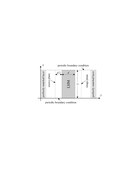
Figure 2: Schematic diagram of two-dimensional (2-D) FDTD simulation domain for calculation of numerical transmission coefficient

For any periodic structures, the field at any time satisfies the Bloch theory, i.e.

$$\textbf{E}(x+L)=\textbf{E}(x)e^{jk_{x}L},~{}~{}~{}~{}\textbf{H}(x+L)=\textbf{H}(x)e^{jk_{x}L},$$ (28)

where $x$ is any location in the computation domain, $k_{x}$ is the wave number in $x$-direction and $L$ is the lattice period along the direction of periodicity. When updating the fields at the boundary of computation domain using the FDTD method, the required fields outside the computation domain can be calculated using known field values inside the domain through (28). Since infinite structures can be truncated with any period, for saving computation time, we have used only four FDTD cells in $x$-direction ($L=4\Delta x$). Along $y$-direction, the Berenger’s original perfectly matched layer (PML) [37] is used for absorbing propagating waves ($k_{x}<k_{0}$), and the modified PML [38] is used when calculating the transmission coefficient for evanescent waves ($k_{x}>k_{0}$). A soft plane-wave sinusoidal source (which allows scattered waves to pass through) with phase delay corresponding to different wave number is used for excitations,

$$H_{z}\left(i,j_{s}\right)=H_{z}\left(i,j_{s}\right)+s(t)e^{-jk_{x}i\Delta x},$$ (29)

where $j_{s}$ is the location of source along $y$-direction, $s(t)$ is a time domain sinusoidal wave function, $i\in\left[1,I\right]$ is the index of cell location and $I$ is the total number of cells in $x$-direction ($I=4$ in our case). By changing the values of wave number $k_{x}$, either pure propagating waves ($k_{x}<k_{0}$) or pure evanescent waves ($k_{x}>k_{0}$) can be excited.

The spatial resolution in FDTD simulations is $\Delta x=\Delta y=\lambda/100$ where $\lambda$ is the free space wavelength at the operating frequency. According to the stability criterion [3], the discretised time step is $\Delta t=\Delta x/\sqrt{2}c$ where $c$ is the speed of light in the free space. As illustrated in Fig. 2, the source plane is located at a distance of $d/2$ to the front interface of the LHM slab where $d$ is the thickness of the slab. Therefore the first image plane is at the centre of the LHM slab and the second image plane is at the same distance of $d/2$ beyond the slab. The spatial transmission coefficient is calculated as a ratio of the field intensity at the second image plane to the source plane for different transverse wave numbers $k_{x}$ after the steady-state is reached in simulations.

Figure 3 shows the transmission coefficient for an infinite planar LHM slab with thickness $d=0.2\lambda$ calculated using the FDTD method with and without averaging of permittivity along the boundaries, and its comparison with exact analytical solutions.

Figure 3: Comparison of transmission coefficient of infinite planar LHM slabs calculated from exact analytical solutions and dispersive FDTD method with and without averaging of permittivity along the boundaries of LHM slabs.

It can be seen that using the arithmetic mean of permittivity, the numerical results show excellent agreement with analytical solution using spatial resolution $\Delta x=\lambda/100$. Good correspondence can be also obtained when the FDTD cell size is increased to $\Delta x=\lambda/80$. On the other hand, without averaging, the material boundary is not correctly modelled which introduces an amplification (resonance) at a location of approximately $k_{x}=2.4k_{0}$ in transmission coefficient for the case of $\Delta x=\lambda/100$. Reducing FDTD cell size to $\Delta x=\lambda/200$ and $\Delta x=\lambda/400$, the behaviour of the resonance remains similar but the location shifts to $k_{x}=2.8k_{0}$ and $k_{x}=3.2k_{0}$, respectively. Therefore we predict that only if a very small FDTD cell size is used in simulations that the results can converge to the right solution. Such a comparison demonstrates the significance of the averaging technique. Conventionally the arithmetic averaging is only a second-order correction for modelling of conventional dielectric slabs, however it is shown in Fig. 3 that for modelling of LHM slabs, the averaging becomes an essential modification.

The results shown in Fig. 3 may explain some incorrect results obtained previously. For instance, the amplification of transmission coefficient in [26, 27] is caused by incorrect modelling of material boundaries, but such amplification is pure numerical and does not exist in actual LHM slabs [34, 33]. It is claimed in [39] that the imaging property of finite-sized LHM slabs is significantly affected by their transverse dimensions, which we suppose that the conclusion is drawn from incorrect numerical simulations. We have performed accurate simulations using averaging of material properties and confirmed that the resolution of a near-field lens using LHMs is free from its transverse aperture size [30].

In our simulations for the calculation of transmission coefficient, we have used PBCs in $x$-direction to model infinite structures and averaged permittivity along the boundaries in $y$-direction. If one requires to model finite-sized structures (in both $x$- and $y$-directions), the averaged permittivity/permeability needs to be used for the corresponding tangential component along the boundaries in both directions.

Besides the averaging technique used along the boundaries of LHM slabs, there are other numerical aspects in FDTD simulations in order to model the behaviour of LHM slab correctly and accurately. These aspects are introduced respectively in following sections.

4 Effects of Numerical Material Parameters

Usually for modelling of conventional dielectrics, the results are assumed to be accurate enough i.e. the effect of numerical material parameters can be ignored if an FDTD cell size of smaller than $\Delta x=\lambda/20$ is used. However since the discretisation introduces a mismatch between numerical and analytical permittivity/permeability, when modelling LHMs, especially when the evanescent waves are involved, the FDTD spatial resolution has a significant impact on the accuracy of simulation results. The effect of numerical permittivity/permeability is originally reported in [28] for lossless LHMs using the (E, J, H, M) scheme. Following the same procedure one can also obtain the numerical permittivity/permeability for the case of lossy LHMs. In this paper, the numerical permittivity/permeability (for lossy LHMs) is derived for the (E, D, H, B) scheme.

In the case of plane waves, when

$$\textbf{E}^{n}=\textbf{E}e^{jn\omega\Delta t},~{}~{}~{}~{}\textbf{D}^{n}=\textbf{D}e^{jn\omega\Delta t},$$ (30)

Eq. (13) reduces to $\textbf{D}^{n}=\tilde{\varepsilon}\textbf{E}^{n}$, where $\tilde{\varepsilon}$ is the numerical permittivity of the following form:

$$\tilde{\varepsilon}=\varepsilon_{0}\left[1-\frac{\omega^{2}_{p}(\Delta t)^{2}\cos^{2}\frac{\omega\Delta t}{2}}{2\sin\frac{\omega\Delta t}{2}\left(2\sin\frac{\omega\Delta t}{2}-j\gamma\Delta t\cos\frac{\omega\Delta t}{2}\right)}\right].$$ (31)

If the collision frequency $\gamma=0$, then (31) reduces to the numerical permittivity for lossless LHMs given in [28].

Previously we have used an FDTD cell size of $\Delta x=\lambda/100$ in simulations. Substitute the corresponding time step $\Delta t=\Delta x/\sqrt{2}c$ and the operating frequency, we can obtain the numerical relative permittivity from (31) as $\tilde{\varepsilon}_{r}=-0.9993-0.0010j$. Although there is a mismatch between the real part of relative permittivity and $-1$, the loss in LHMs damps such a mismatch and the simulation results show very good accuracy. However if we increase FDTD cell size, the numerical permittivity introduces severer mismatch which causes the discrepancy between FDTD simulation result and exact solutions. For example, for the case of $\Delta x=\lambda/40$, the mismatch brings an amplification in transmission coefficient as shown in Fig. 4.

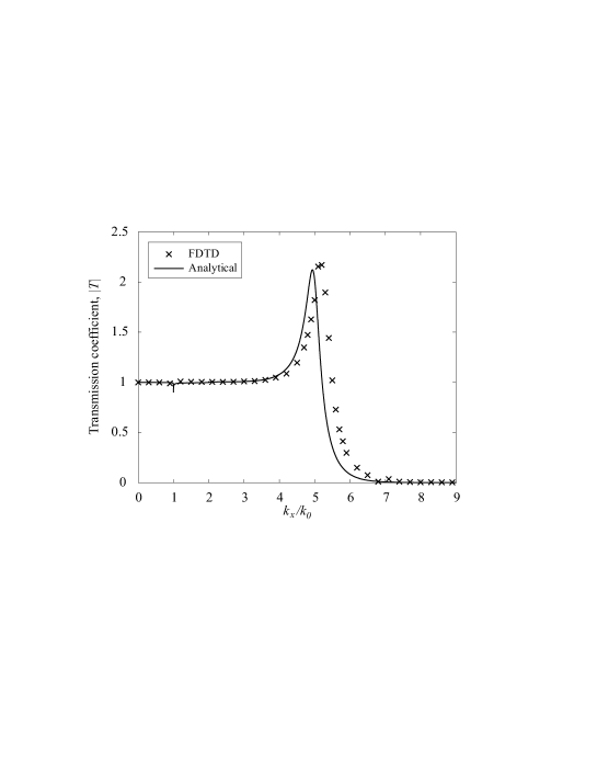
Figure 4: Transmission coefficient of infinite planar LHM slabs using the proposed FDTD method with averaged permittivity and without the correction of material parameters. The amplification of transmission coefficient is caused by the mismatch introduced by the time discretisation in FDTD ($\varepsilon_{r}=-0.9959-0.0010j$) with $\Delta x=\lambda/40$. The same permittivity is used to obtain the analytical solution for comparison.

Again using (31) we can estimate this mismatch and the numerical relative permittivity reads $\tilde{\varepsilon}_{r}=-0.9959-0.0010j$. Using such permittivity in analytical formulations, we can obtain the corresponding transmission coefficient which is also plotted in Fig. 4 for comparison. A good correspondence is shown and at high-wave-vector region, the discrepancy is cause by insufficient sampling points as for the case of using large cell size (e.g. $\Delta x>\lambda/10$) for conventional FDTD.

Another advantage of estimating the numerical permittivity is the correction of the mismatch for FDTD simulations. After simple derivations, we can obtain corrected plasma frequency and collision frequency as

$$\tilde{\omega}^{2}_{p} = \frac{2\sin\frac{\omega\Delta t}{2}\left[-2(\varepsilon^{\prime}_{r}-1)\sin\frac{\omega\Delta t}{2}-\varepsilon^{\prime\prime}_{r}\gamma\Delta t\cos\frac{\omega\Delta t}{2}\right]}{(\Delta t)^{2}\cos^{2}\frac{\omega\Delta t}{2}},$$

$$\tilde{\gamma} = \frac{2\varepsilon^{\prime\prime}_{r}\sin\frac{\omega\Delta t}{2}}{(\varepsilon^{\prime}_{r}-1)\Delta t\cos\frac{\omega\Delta t}{2}},$$ (32)

where $\varepsilon^{\prime}_{r}$ and $\varepsilon^{\prime\prime}_{r}$ are the real and imaginary parts of the design relative permittivity $\varepsilon_{r}$, respectively. For the case of $\varepsilon_{r}=-1-0.001j$, substitute $\varepsilon^{\prime}_{r}=-1$ and $\varepsilon^{\prime\prime}_{r}=-0.001$ into (32) we get $\tilde{\omega}_{p}=1.4157\omega$ and $\tilde{\gamma}=5.0051\times 10^{-4}\omega$. Using the corrected material parameters, the FDTD simulation result and its comparison with analytical solutions are shown in Fig. 5.

Figure 5: Transmission coefficient of infinite planar LHM slabs using the proposed FDTD method with averaged permittivity and with the correction of material parameters. The numerical permittivity in FDTD ($\Delta x=\lambda/40$) is $\varepsilon_{r}=-1-0.001j$. The same permittivity is used to obtain the analytical solution for comparison.

It can be seen that the mismatch has been canceled in FDTD simulations hence there is no amplification in transmission coefficient. Again the discrepancy with exact solutions in high-wave-vector region is caused by insufficient sampling points for such an FDTD spatial resolution of $\Delta x=\lambda/40$. Therefore we suggest to use FDTD cell size smaller than $\Delta x=\lambda/80$ for modelling of LHMs especially when evanescent waves are involved.

5 Effects of Switching Time

Conventionally for single frequency simulations, the source should be smoothly switched to its maximum value in order to avoid exciting other frequency components [23]. For modelling of LHMs, the switching time has even more significant effect on their behaviour. It is well known that the switching time considerably influences the oscillation of images and often thirty period is used as the switching time [25, 27]. However, perhaps this is the reason that no stable images could be obtained in [23, 27] since recently, it is reported in [40] that using a switching time of at least one hundred periods one can obtain stabilised image for lossless LHMs.

In our FDTD simulations, we also notice that switching time influences the oscillation of the field intensity at the image plane and hence the convergence time in simulations. We have performed FDTD simulations with different switching time equal to $50T_{0}$, $150T_{0}$ and $250T_{0}$ where $T_{0}$ is the period of the sinusoidal signal. The FDTD cell size is $\Delta x=\lambda/100$ and corrected material parameters from (32) are used. In order to ensure faster convergence, we have chosen larger amount of losses and used $\tilde{\varepsilon}_{r}=-1-0.01j$ in simulations. It should be noted that because high-wave-vector components travel very slowly in LHM slabs and the process of the growth of evanescent waves requires a very long time to reach the steady-state, field values should be taken only after total convergence is reached in simulations. For our case of $\tilde{\varepsilon}_{r}=-1-0.01j$, we have used a criteria of 0.001% for detecting iteration errors and terminating simulations. It is clearly shown in Fig. 6 that for a fixed wave number ($k_{x}=3k_{0}$), the oscillation of field intensity can be significantly suppressed by prolonging the switching time.

Figure 6: The influence of different switching time on the convergence time in FDTD simulation of infinite LHM slabs for a fixed wave number $k_{x}=3k_{0}$. The $T_{0}$ is the period of the sinusoidal wave function at the operating frequency. The field intensity is taken at the second image plane of the LHM slab.

It is understandable that when the oscillation can be neglected, the convergence time increases with the switching time. For demonstration of the impact of switching time on convergence time, we have performed FDTD simulations with various switching time. The collected data is plotted in Fig. 7.

Figure 7: The dependence of the convergence time on the switching time in FDTD simulations of infinite LHM slabs for a fixed wave number $k_{x}=3k_{0}$. A criteria of 0.001% is used to detect iteration errors and terminating simulations.

It can be seen that there exists an optimum switching time when the minimum convergence time can be achieved for the case of $k_{x}=3k_{0}$. However for different wave vectors and different material parameters, the behaviour of oscillation differs considerably and in certain cases the oscillation may last until a very long time. For practical simulations such as modelling of subwavelength imaging by a line source, since the source contains all wave vectors, therefore it is necessary to switch the source slowly enough to ensure and speed up the convergence of simulations.

6 Conclusions

In conclusion, we have performed simulations of LHMs using the dispersive FDTD method. Two ADE methods namely the (E, D, H, B) scheme and the (E, J, H, M) scheme which lead to exactly same results and the respective averaging techniques along material boundaries are introduced. The comparison with exact analytical solutions demonstrates that the averaging of permittivity/permeability along the boundaries of LHM slabs is essential for correct and accurate modelling of LHMs. The numerical permittivity in FDTD is formulated where a mismatch between numerical and analytical permittivity is introduced by FDTD time discretisation. We suggest to correct such a mismatch in order to model LHMs with their desired parameters in FDTD. The behaviour of oscillation of field intensity for different switching time is also analysed. It is shown that there exists an optimum value which leads to fast convergence in simulations.

References

References

- [1] V. G. Veselago, “The electrodynamics of substances with simultaneously negative value of and ,” Sov. Phys. Usp., vol. 10, pp. 509, 1968.
- [2] J. B. Pendry, “Negative refraction makes a perfect lens,” Phys. Rev. Lett., vol. 85, pp. 3966, 2000.
- [3] A. Taflove, Computational Electrodynamics: The Finite-Difference Time-Domain Method, 2nd ed., Artech House, Norwood, MA, 2000.
- [4] R. Luebbers, F. P. Hunsberger, K. Kunz, R. Standler, and M. Schneider, “A frequency-dependent finite-difference time-domain formulation for dispersive materials”, IEEE Trans. Electromagn. Compat., vol. 32, pp. 222-227, Aug. 1990.
- [5] O. P. Gandhi, B.-Q. Gao, and J.-Y. Chen, “A frequency-dependent finite-difference time-domain formulation for general dispersive media,” IEEE Trans. Microwave Theory Tech., vol. 41, pp. 658-664, Apr. 1993.
- [6] D. M. Sullivan, “Frequency-dependent FDTD methods using Z transforms,” IEEE Trans. Antennas Propagat., vol. 40, pp. 1223-1230, Oct. 1992.
- [7] R. J. Luebbers, F. Hunsberger, and K. S. Kunz, “A frequency-dependent finite-difference time-domain formulation for transient propagation in plasma,” IEEE Trans. Antennas Propagat., vol. 39, no. 1, pp. 29-34, 1991.
- [8] R. J. Luebbers and F. Hunsberger, “FDTD for Nth-order dispersive media,” IEEE Trans. Antennas Propagat., vol. 40, no. 11, pp. 1297-1301, 1992.
- [9] F. Hunsberger, R. J. Luebbers, and K. S. Kunz, “Finite-difference time-domain analysis of gyrotropic media. I: Magnetized plasma,” IEEE Trans. Antennas Propagat., vol. 40, no. 12, pp. 1489-1495, 1992.
- [10] C. Melon, P. Leveque, T. Monediere, A. Reineix, and F. Jecko, “Frequency dependent finite-difference-time-domain formulation applied to ferrite material,” Microwave Opt. Technol. Lett., vol. 7, no. 12, pp. 577-579, 1994.
- [11] A. Akyurtlu and D. H. Werner, “BI-FDTD: a novel finite-difference time-domain formulation for modeling wave propagation in bi-isotropic media,” IEEE Trans. Antennas Propagat., vol. 52, no. 2, pp. 416-425, 2004.
- [12] A. Grande, I. Barba, A. Cabeceira, J. Represa, P. So, and W. Hoefer, “FDTD modeling of transient microwave signals in dispersive and lossy bi-isotropic media,” IEEE Trans. Microwave Theory Tech., vol. 52, no. 3, pp. 773-784, 2004.
- [13] A. Akyurtlu and D. H. Werner, “A novel dispersive FDTD formulation for modelling transient propagation in chiral metamaterials,” IEEE Trans. Antennas Propagat., vol. 52, no. 9, pp. 2267-2276, 2004.
- [14] J.-Y. Lee, J.-H. Lee. H.-S. Kim, N.-W. Kang and H.-K. Jung, “Effective medium approach of left-handed material using a dispersive FDTD method,” IEEE Trans. Magnetics, vol. 41, no. 5, pp. 1484-1487, 2005.
- [15] T. Kashiwa, N. Yoshida, and I. Fukai, “A treatment by the finite-difference time-domain method of the dispersive characteristics associated with orientation polarization,” Trans. IEICE, vol. E73, no. 8, pp. 1326-1328, 1990.
- [16] T. Kashiwa and I. Fukai, “A treatment by the FD-TD method of the dispersive characteristics associated with electronic polarization,” Microwave Opt. Technol. Lett., vol. 3, no. 6, pp. 203-205, 1990.
- [17] P. M. Goorjian and A. Taflove, “Direct time integration of Maxwell’s equations in nonlinear dispersive media for propagation and scattering of femtosecond electromagnetic solitons,” Optics Lett., vol. 17, no. 3, pp. 180-182, 1992.
- [18] O. P. Gandhi, B. Q. Gao, and J. Y. Chen, “A frequency-dependent finite-difference time-domain formulation for induced current calculations in human beings,” Bioelectromagnetics, vol. 13, no. 6, pp. 543-556, 1992.
- [19] O. P. Gandhi, B. Q. Gao, and J. Y. Chen, “A frequency-dependent finite-difference time-domain formulation for general dispersive media,” IEEE Trans. Microwave Theory Tech., vol. 41, no. 4, pp. 658-665, 1993.
- [20] L. Lu, Y. Hao, and C. Parini, “Dispersive FDTD characterisation of no phase-delay radio transmission over layered left-handed meta-materials structure,” IEE Proceedings-Science Measurement and Technology, 151 (6): 403-406 Nov 2004.
- [21] D. M. Sullivan, “Nonlinear FDTD formulations using Z transforms,” IEEE Trans. Microwave Theory Tech., vol. 43, no. 3, pp. 676-682, 1995.
- [22] V. Demir, A. Z. Elsherbeni, and E. Arvas, “FDTD formulation for dispersive chiral media using the Z transform method,” IEEE Trans. Antennas Propagat., vol. 53, no. 10, pp. 3374-3384, 2005.
- [23] R. W. Ziolkowski and E. Heyman, “Wave propagation in media having negative permittivity and permeability,” Phys. Rev. E, vol. 64, pp. 056625, 2001.
- [24] P. F. Loschialpo, D. L. Smith, D. W. Forester, F. J. Rach- ford, and J. Schelleng, “Electromagnetic waves focused by a negative-index planar lens,” Phys. Rev. E, vol. 67, pp. 025602, 2003.
- [25] S. A. Cummer, “Simulated causal subwavelength focusing by a negative refractive index slab,” Appl. Phys. Lett., vol. 82, pp. 1503, 2003.
- [26] M. W. Feise and Y. S. Kivshar, “Sub-wavelength imaging with a left-handed material flat lens,” Phys. Lett. A, vol. 334, pp. 326, 2005.
- [27] X. S. Rao and C. K. Ong, “Subwavelength imaging by a left-handed material superlens,” Phys. Rev. E, vol. 68, pp. 067601, 2003.
- [28] J. J. Chen, T. M. Grzegorczyk, B.-I.Wu, and J. A. Kong, “Limitation of FDTD in simulation of a perfect lens imaging system,” Opt. Express, vol. 13, pp. 10840, 2005.
- [29] M. W. Feise, J. B. Schneider, and P. J. Bevelacqua, “Finite-difference and pseudospectral time-domain methods applied to backward-wave metamaterials,” IEEE Trans. Antennas Propagat., vol. 52, pp. 2955, 2004.
- [30] Y. Zhao, P. Belov, and Y. Hao, “Accurate modelling of the optical properties of left-handed media using a finite-difference time-domain method,” submitted to Phys. Rev. Lett. (cond-mat/0610301) (2006).
- [31] A. Mohammadi, H. Nadgaran, and M. Agio, “Contour-path effective permittivities for the two-dimensional finite-difference time-domain method,” Opt. Express, vol. 13, pp. 10367-10381, 2005.
- [32] A. Mohammadi, and M. Agio, “Dispersive contour-path finite-difference time-domain algorithm for modelling surface plasmon polaritons at flat interfaces,” Opt. Express, vol. 14, pp. 11330-11338, 2006.
- [33] V. A. Podolskiy and E. E. Narimanov, “Near-sighted superlens,” Opt. Lett., vol. 30, pp. 75, 2005.
- [34] D. R. Smith, D. Schurig, M. Rosenbluth, S. Schultz, S. A. Ramakrishna, and J. B. Pendry, “Limitations on subdiffraction imaging with a negative refractive index slab,” Appl. Phys. Lett., vol. 82, pp. 1506, 2003.
- [35] F. B. Hildebrand, Introduction to Numerical Analysis. New York: Mc-Graw-Hill, 1956.
- [36] K.-P. Hwang and A. C. Cangellaris, “Effective permittivities for second-order accurate FDTD equations at dielectric interfaces,” IEEE Microw. Wireless Components Lett., vol. 11, pp. 158, 2000.
- [37] J. R. Berenger, “A perfectly matched layer for the absorption of electromagnetic waves,” J. Computat. Phys., vol. 114, pp. 185, 1994.
- [38] J. Fang and Z. Wu, “Generalised perfectly matched layer for the absorption of propagating and evanescent waves in lossless and lossy media,” IEEE Trans. Microw. Theory Tech., vol. 44, pp. 2216, 1996.
- [39] L. Chen, S. He, and L. Shen, “Finite-size effects of a left-handed material slab on the image quality,”, Phys. Rev. Lett., vol. 92, pp. 107404, 2004.
- [40] X. Huang and L. Zhou, “Modulating image oscillations in focusing by a metamaterial lens: time-dependent Green’s function approach,” Phys. Rev. B, vol. 74, pp. 045123, 2006.