Quasi-Classical Calculation of the Mixed-State Thermal Conductivity
in $s$-Wave and $d$-Wave Superconductors

Abstract

To see how superconducting gap structures affect the longitudinal component of mixed-state thermal conductivity $\kappa_{xx}(B)$, the magnetic-field dependences of $\kappa_{xx}(B)$ in $s$-wave and $d$-wave superconductors are investigated. Calculations are performed on the basis of the quasi-classical theory of superconductivity by fully taking account of the spatial variation of the normal Green’s function, neglected in previous works, by the Brandt-Pesch-Tewordt approximation. On the basis of our result, we discuss the possibility of $\kappa_{xx}(B)$ measurement as a method of probing the gap structure.

1 Introduction

In the last two decades, several new superconductors showing unconventional pairing properties have been found among heavy-fermion, oxide, and organic materials. [1] These discoveries have motivated studies on identifying the gap symmetry, as well as clarifying the mechanism of the superconductivity. At present, it has been well established that bulk measurements of mixed-state thermodynamic quantities can provide important information on the gap structure.  [2, 3, 4, 5, 6, 7] The principle behind this technique is that the low-energy quasiparticles around vortex cores, relevant to the low-temperature thermodynamics, sensitively reflect the structure of the superconducting gap. On the basis of the numerical solution of quasi-classical Eilenberger equations, we have demonstrated that the gap structure can be inferred from the low-temperature field dependence [8, 9] and field-angle dependence [10, 11, 12, 13] of the specific heat and magnetization.

Thermal-transport measurement in a superconducting mixed state is another option for such a spectroscopic method based on the bulk property of a sample. At very low temperatures, where the transport property is mainly determined by the elastic impurity scattering, the thermal conductivity can also provide important information on the pairing state. Roughly speaking, the longitudinal component of mixed-state thermal conductivity $\kappa_{xx}(B)$ at zero temperature is given by $\kappa_{xx}(B)\sim\langle v_{x}^{2}N_{\mib{p}}(0)\tau^{\rm tr}_{\mib{p}}(0)\rangle$, where $N_{\mib{p}}(0)$ is the momentum-resolved density of states at the Fermi surface, $v_{x}$ is the $x$-component of the Fermi velocity, $\tau^{\rm tr}_{\mib{p}}(0)$ is the momentum-dependent transport lifetime, and $\langle\cdots\rangle$ denotes the average over the Fermi surface (see eq. (34) below). As Volovik [3] pointed out, $N_{\mib{p}}(0)$ and $\tau^{\rm tr}_{\mib{p}}(0)$ in a nodal superconductor are modified by the field-induced Doppler shift on the delocalized quasiparticles, while in an $s$-wave superconductor, such an effect is negligibly small. Hence, we expect that the behavior of $\kappa_{xx}(B)$ in a nodal superconductor is different from that in an $s$-wave superconductor. Recently, a series of mixed-state thermal-transport experiments have been extensively performed by Matsuda’s group to determine the gap structures in several newly found superconductors. [14]

The low-temperature mixed-state thermal transport is mainly determined by the following three mechanisms: impurity scattering, giving the Drude thermal conductivity in the normal state; Andreev scattering by vortex cores; [15] and the Doppler shift due to the supercurrents. [16] So far, there have been several approaches to the calculation of the mixed-state thermal conductivity in a moderately clean superconductor.  [17, 18, 19, 20, 21, 22, 23, 24, 25, 26, 27, 28] Among them, two approximations have been frequently used. One is the Doppler shift approximation. [22, 23] This method neglects the Andreev scattering by vortex cores, and thus is valid only near the lower critical field $H_{c1}$. The other approximation [19, 25] is based on the Brandt-Pesch-Tewordt (BPT) approximation. [29, 30] The latter is superior to the former in that it takes account of both the Doppler shift and the vortex-core scattering. In the BPT approximation, however, the spatial variation of the normal Green’s function is neglected, which is strongly related to the local density of states detected by the scanning tunneling microscopy experiment. [31] Hence, this approximation is valid only near the upper critical field $H_{c2}$. At present, there is no theoretical work valid in the wide field range from $H_{c1}$ to $H_{c2}$. In view of analyzing the experimental data for several newly found superconductors, it is of importance to calculate the mixed-state thermal conductivity beyond these two approximations.

It is well known that the quasi-classical theory of superconductivity [32, 33] can accurately describe the mixed-state properties in a wide field range from $H_{c1}$ to $H_{c2}$. The advantage of this framework is that, if applied to the calculation of mixed-state thermal conductivity, it can take account of the spatial variation of the normal Green’s function neglected in the BPT approximation, as well as the Andreev vortex scattering neglected in the Doppler shift approximation. Of course, we need to solve a set of transport-like equations to accomplish the computation.

In this work, we adopt the quasi-classical theory of superconductivity, and develop a method of calculating the mixed-state thermal conductivity $\kappa_{xx}(B)$. Then, we apply our analysis to two-dimensional $s$-wave and $d$-wave superconductors, and calculate the magnetic-field dependences of $\kappa_{xx}(B)$ to clarify the effect of the gap structure on the mixed-state thermal transport. We also study the effect of the in-plane Fermi surface anisotropy. On the basis of our result, we discuss the possibility of using $\kappa_{xx}(B)$ as a method of probing the gap structure.

The paper is organized as follows. In §2, we develop a method of calculating the mixed-state thermal conductivity based on the quasi-classical theory of superconductivity. In §3, we present our numerical results for the mixed-state thermal conductivity obtained by solving the quasi-classical equations. We discuss our result in §4, and conclude in §5. We use the unit $\hbar=c=k_{\rm B}=1$ throughout this paper.

2 Formulation

2.1 Linear-response-equation

Our approach to mixed-state thermal transport is based on the Kubo formula for a homogeneous temperature gradient. [34] Then, the mixed-state thermal conductivity $\kappa_{xx}(B)$ is given by

$$\kappa_{xx}(B)=-\frac{1}{T}{\rm Im}\left.\frac{Q^{R}_{xx}(\omega)}{\omega}\right|_{\omega\to 0},$$ (1)

where $Q^{R}_{xx}$ is obtained from the (Matsubara) heat-current correlation function

$$Q_{xx}({\rm i}\omega_{m}) = \frac{1}{V}\int d^{2}r_{1}d^{2}r_{2}\int_{0}^{T^{-1}}d\tau e^{{\rm i}\omega_{m}\tau}$$ (2)

$$\times\Big{(}-\big{\langle}T_{\tau}[J_{x}(\mib{r}_{1},\tau)J_{x}(\mib{r}_{2},0)]\big{\rangle}_{\rm eq}\Big{)},$$

after the analytical continuation $Q_{xx}^{R}(\omega)=Q_{xx}({\rm i}\omega_{m}\to\omega+{\rm i}0_{+})$. Here, $\omega_{m}=2\pi Tm$ are bosonic Matsubara frequencies, $\langle\cdots\rangle_{\rm eq}$ denotes the statistical average, and $V$ is the volume of the sample. The heat-current operator $\mib{J}$ in the real-time representation is given by

$$\mib{J}({\it 1}) = -\frac{1}{2m}\sum_{\rm spin}\Big{[}\partial_{t_{1}}\big{(}\mib{\nabla}_{r_{2}}+{\rm i}|e|\mib{A}({\it 2})\big{)}$$ (3)

$$\left.\quad+\big{(}\mib{\nabla}_{r_{1}}-{\rm i}|e|\mib{A}({\it 1})\big{)}\partial_{t_{2}}\Big{]}\psi^{\dagger}({\it 1})\psi({\it 2})\right|_{{\it 2}\to{\it 1}},$$

where $\psi$ is the electron-field operator and ${\it 1}=(\mib{r}_{1},t_{1}),{\it 2}=(\mib{r}_{2},t_{2})$. To evaluate $Q_{xx}$, we follow the procedure suggested by Klimesch and Pesch. [35] They showed that the heat-current correlation function can be constructed in a manner similar to obtaining the density correlation function $D$ under charge disturbance. On the imaginary (Matsubara) axis, $D$ is given by

$$D({\rm i}\omega_{m}) = \frac{1}{V}\int d^{2}r_{1}d^{2}r_{2}\int_{0}^{T^{-1}}d\tau e^{{\rm i}\omega_{m}\tau}$$ (4)

$$\times\Big{(}-\big{\langle}T_{\tau}[n(\mib{r}_{1},\tau)n(\mib{r}_{2},0)]\big{\rangle}_{\rm eq}\Big{)},$$

where $n=\sum_{\rm spin}\psi^{\dagger}\psi$ is the electron density. The procedure by Klimesch and Pesch is justified as long as we consider a moderately clean superconductor $\xi_{0}/l\ll 1$ (coherence length $\xi_{0}$ and mean free path $l$), where the impurity vertex corrections for the heat current can be safely neglected. When we consider a dirtier superconductor, we have to include the vertex corrections to satisfy the conservation of the energy density. [36, 37, 38] A full quasi-classical treatment for the charge current that includes the impurity vertex corrections can be found in ref. Eschrig. Note that the present result can be also derived from the Keldysh technique. [40]

Let us briefly review the procedure used by Klimesch and Pesch [35] to find the connection between the heat-current correlation function $Q_{xx}$ and the density correlation function $D$. Consider an external scalar potential $\Phi=-|e|\phi$ that couples to the electron density ${n}$. Next, we define the quasi-classical Green’s function as

$$\widehat{g}=\int\frac{d\zeta_{\mib{p}}}{{\rm i}\pi}\left({G\atop-F^{{\dagger}}}{F\atop-G}\right),$$ (5)

where $G$, $F$, and $F^{{\dagger}}$ are the normal and anomalous Green’s functions in the Gor’kov formalism, and $\zeta_{\mib p}$ is the single-particle energy measured from the Fermi energy. We divide this Green’s function into two parts, $\widehat{g}=\widehat{g}_{0}+\delta\widehat{g}$, where

$$\widehat{g}_{0}=\left({g_{0}\atop{\rm i}f_{0}^{{\dagger}}}{-{\rm i}f_{0}\atop-g_{0}}\right)$$ (6)

is the static part, and

$$\delta\widehat{g}=\left({g_{1}\atop-f_{2}}{f_{1}\atop g_{2}}\right)$$ (7)

is the linear-response part. Then, using the Kubo formula for the charge disturbance, we obtain an expression for $D$ within the quasi-classical accuracy,

$$D({\rm i}\omega_{m})={\rm i}2\pi N_{\rm F}T\sum_{\varepsilon_{n}}\Big{\langle}\widetilde{g_{1}}\Big{\rangle},$$ (8)

where $\widetilde{g_{1}}={g_{1}}/{\Phi}$, and $N_{\rm F}$ is the density of states in the normal state. Here we neglected the contribution far from the Fermi surface. [41] On the other hand, by a direct evaluation of the density correlation function in the Gor’kov formalism, we obtain, within the quasi-classical accuracy, [42]

$$D({\rm i}\omega_{m})={\rm i}2\pi N_{\rm F}T\sum_{\varepsilon_{n}}\Big{\langle}\int\frac{d\zeta_{\mib{p}}}{{\rm i}\pi}(G_{0}G_{0}-F_{0}F_{0}^{\dagger})\Big{\rangle},$$ (9)

in which we introduce a shorthand notation $G_{0}G_{0}-F_{0}F_{0}^{\dagger}=G_{0}({\rm i}\varepsilon_{n}+{\rm i}\omega_{m})G_{0}({\rm i}\varepsilon_{n})-F_{0}({\rm i}\varepsilon_{n}+{\rm i}\omega_{m})F_{0}^{{\dagger}}({\rm i}\varepsilon_{n})$. $G_{0}$, $F_{0}$, and $F_{0}^{{\dagger}}$ are the static components of the Green’s function in the Gor’kov formalism. Note that, as mentioned before, we neglect the impurity vertex corrections in this work. We also neglect the vortex motion, and consider only the quasiparticle contribution. Then, by comparing the above two equations, we obtain the following relation,

$$\widetilde{g_{1}}=\int\frac{d\zeta_{\mib{p}}}{{\rm i}\pi}(G_{0}G_{0}-F_{0}F_{0}^{\dagger}).$$ (10)

Next, we apply the same calculation scheme to the thermal conductivity $\kappa_{xx}(B)$. By a direct evaluation of the heat-current correlation function in the Gor’kov formalism, we obtain within the quasi-classical accuracy,

$$Q_{xx}({\rm i}\omega_{m}) = -{\rm i}2\pi N_{\rm F}T\sum_{\varepsilon_{n}}\Big{\langle}v_{x}^{2}(\varepsilon_{n}+\frac{1}{2}\omega_{m})^{2}$$ (11)

$$\hskip 28.45274pt\times\int\frac{d\zeta_{\mib{p}}}{{\rm i}\pi}(G_{0}G_{0}-F_{0}F_{0}^{\dagger})\Big{\rangle}.$$

From the last two equations, we can express $Q_{xx}$ in terms of $\delta\widehat{g}$ as

$$Q_{xx}({\rm i}\omega_{m})=-{\rm i}2\pi N_{\rm F}T\sum_{\varepsilon_{n}}\Big{\langle}v_{x}^{2}(\varepsilon_{n}+\frac{1}{2}\omega_{m})^{2}\;\widetilde{g_{1}}\Big{\rangle}.$$ (12)

The quantity $\delta\widehat{g}$ is determined by the linear-response equation: [43, 44]

$$\mib{v}\cdot\mib{\nabla}\delta\widehat{g}+\varepsilon_{n+}\widehat{\tau}_{3}\delta\widehat{g}-\varepsilon_{n}\delta\widehat{g}\widehat{\tau}_{3}+{\rm i}\Big{[}|e|\mib{v}\cdot\mib{A}\widehat{\tau}_{3}-\widehat{\Delta},\delta\widehat{g}\Big{]}_{-}$$

$$+\frac{1}{2\tau}\langle\widehat{g}_{0}({\rm i}\varepsilon_{n+})\rangle\delta\widehat{g}-\delta\widehat{g}\frac{1}{2\tau}\langle\widehat{g}_{0}({\rm i}\varepsilon_{n+})\rangle$$

$$=\widehat{g}_{0}({\rm i}\varepsilon_{n+}){\rm i}\Phi-{\rm i}\Phi\widehat{g}_{0}({\rm i}\varepsilon_{n}),$$ (13)

where $\varepsilon_{n+}=\varepsilon_{n}+\omega_{m}$, $[A,B]_{-}=AB-BA$, and $\widehat{\tau}_{3}=({1\atop 0}{0\atop-1})$. In the above equation, we assumed Born scattering for convenience, and unitarity scattering will be discussed later. Eq. (13) is supplemented by the normalization condition,

$$\widehat{g}_{0}({\rm i}\varepsilon_{n+})\delta\widehat{g}+\delta\widehat{g}\,\widehat{g}_{0}({\rm i}\varepsilon_{n})=0.$$ (14)

The static part of the quasi-classical Green’s function $\widehat{g}_{0}$ satisfies the following static (or Eilenberger) equation,

$$\mib{v\cdot\nabla}\widehat{g}_{0}+\Big{[}\varepsilon_{n}\widehat{\tau}_{z}+\langle\widehat{g}_{0}\rangle/2\tau+{\rm i}|e|\mib{v\cdot A}-{\rm i}\widehat{\Delta},\widehat{g}_{0}\Big{]}_{-}=0,$$ (15)

with the normalization condition $\widehat{g}_{0}^{2}=\widehat{1}$. Here, $\widehat{\Delta}(\mib{p},\mib{r})=({0\atop-\Delta^{*}_{\mib{p}}(\mib{r})}{\Delta_{\mib{p}}(\mib{r})\atop 0})$, and $\langle\cdots\rangle$ denotes the Fermi surface average.

Once $\delta\widehat{g}$ is obtained, $\kappa_{xx}(B)$ can be calculated from eqs. (1) and (12). The Matsubara-sum in eq. (12) can be transformed into a real frequency integral using the well-known formula $T\sum_{\varepsilon_{n}}f({\rm i}\varepsilon_{n})=\oint\frac{d\varepsilon}{4\pi{\rm i}}{\rm th}(\frac{\varepsilon}{2T})f(\varepsilon)$. Then, we obtain

$$\kappa_{xx}(B)=4N_{\rm F}T\int_{0}^{\infty}\frac{d\varepsilon}{2T}\frac{\left(\frac{\varepsilon}{2T}\right)^{2}}{{\rm\cosh^{2}}\left(\frac{\varepsilon}{2T}\right)}\big{\langle}v_{x}^{2}[-{\rm i}\widetilde{g_{1}}^{R}]_{\rm sp}\big{\rangle},$$ (16)

where $\widetilde{g_{1}}^{R}(\varepsilon)=\widetilde{g_{1}}({\rm i}\varepsilon_{n}\to\varepsilon+{\rm i}0_{+})$, and $[\cdots]_{\rm sp}$ denotes the spatial average. If we perform the low-temperature expansion of the above expression, we have

$$\left.\frac{\kappa_{xx}}{T}\right|_{T\to 0}=\frac{\pi}{3}N_{\rm F}\big{\langle}v_{x}^{2}[-{\rm i}\widetilde{g_{1}}^{R}]_{\rm sp}\big{\rangle}.$$ (17)

Finally note that, as we will show later, the compact result [25] due to the BPT method corresponds to an approximate expression of eq. (16).

2.2 Numerical procedure

To obtain an input quantity $\widehat{g}_{0}$ for the linear-response equation, eq. (13), we have to solve the static equation (15). To do so, we adopt the Riccati parameterization, [45, 46]

$$f_{0}=\frac{2a}{1+ab},\;f^{\dagger}_{0}=\frac{2b}{1+ab},\;g_{0}=\frac{1-ab}{1+ab},$$ (18)

by introducing two functions $a$ and $b$. Then, the static equation is transformed into the following Riccati-type equations:

$$\mib{v}\cdot\mib{\nabla}a = -2(\widetilde{\varepsilon}_{n}+{\rm i}|e|\mib{v}\cdot\mib{A})a+\widetilde{\Delta}_{\mib{p}}-\widetilde{\Delta}_{\mib{p}}^{*}a^{2},$$ (19)

$$\mib{v}\cdot\mib{\nabla}b = 2(\widetilde{\varepsilon}_{n}+{\rm i}|e|\mib{v}\cdot\mib{A})b-\widetilde{\Delta}_{\mib{p}}^{*}+\widetilde{\Delta}_{\mib{p}}b^{2},$$ (20)

where $\widetilde{\varepsilon}_{n}=\varepsilon_{n}+\langle g\rangle/2\tau$, $\widetilde{\Delta}_{\mib p}=\Delta_{\mib p}+\langle f_{0}\rangle/2\tau$, and $\tau$ is the quasiparticle mean free time. The pair potential is expressed as $\Delta_{\mib{p}}(\mib{r})=w_{\mib{p}}\Delta(\mib{r})$ with the order parameter $\Delta(\mib{r})$ and the pairing function $w_{\mib p}$. For a $d$-wave ($s$-wave) superconductor, we use $w_{\mib{p}}=\sqrt{2}(p_{x}^{2}-p_{y}^{2})/p_{\rm F}^{2}$ ($w_{\mib{p}}=1$), with $p_{\rm F}$ being the Fermi momentum.

The numerical procedure used to solve eqs. (19) and (20) is described in ref. Pedja3. Calculations are performed for a two-dimensional superconductor with a hexagonal vortex lattice state. As mentioned before, we consider a moderately clean superconductor $\xi_{0}/l=0.1$, where $\xi_{0}=v_{\rm F}/2\pi T_{c0}$ and $l=v_{\rm F}\tau$, with $v_{\rm F}$ being the Fermi velocity. We initially assume a two-dimensional isotropic Fermi surface, and later we discuss the effect of the Fermi surface anisotropy. We also assume that the superconductor has a large Ginzburg-Landau parameter $\kappa_{\rm GL}\gg 1$ (most of the newly found superconductors satisfy this condition), so that the magnetic field $B$ is assumed to be constant.

First, we determine the order parameter $\Delta({\mib r})$ self-consistently by the following gap equation,

$$\ln\left(\frac{T}{T_{c0}}\right)\Delta({\mib r})=2\pi T\sum_{\varepsilon_{n}>0}\left(\langle w_{\mib{p}}f_{0}\rangle-\frac{\Delta(\mib{r})}{\varepsilon_{n}}\right),$$ (21)

where $T_{c0}$ is the transition temperature at zero field without any impurity. This procedure requires the anomalous Green’s function $f_{0}$, and it is obtained by solving eqs. (19) and (20) on the Matsubara axis. Note that for a $d$-wave superconductor, we set the anomalous self-energy $\langle f_{0}\rangle$ equal to zero. This treatment is consistent with the neglect of the impurity vertex corrections for the heat current, since both quantities vanish in the limit of zero magnetic field. Of course, for an $s$-wave superconductor, we cannot neglect $\langle f_{0}\rangle$, which satisfies the Anderson theorem for pair breaking. [48]

Figure 1: Real-space images of the order parameter in an $s$-wave superconductor, obtained from our self-consistent calculation. ${\mib r}=(x,y)$ and $\Delta({\mib r})$ are normalized by $r_{B}=(2|e|B)^{-1/2}$ and $\Delta_{0}=1.764T_{c0}$, respectively. $|\Delta({\mib r})|$ in a high field [(a)] and a low field [(b)] are shown.

In Fig. 1, we show real-space images of the obtained order parameter $\Delta({\bf r})$ for an $s$-wave superconductor. Near $H_{c2}$ (Fig. 1(a)), vortices overlap with each other. However, upon lowering the field $H\ll H_{c2}$ (Fig. 1(b)), the vortex core radius becomes smaller and smaller than the intervortex spacing. These behaviors can be obtained only after we calculate the order parameter self-consistently. After we determine the order parameter $\Delta({\mib r})$, we solve eqs. (19) and (20) for the real frequency ${\rm i}\varepsilon_{n}\to\varepsilon\pm{\rm i}0_{+}$ to obtain the retarded (advanced) Green’s function. The impurity self-energy is determined self-consistently in this static equation. [47]

Next we solve the linear-response equation. To calculate $\kappa_{xx}(B)$ using eq. (16), we need to carry out the analytical continuation of eq. (13) to real frequencies. The off-diagonal components of $\delta\widehat{g}$ can be eliminated by the normalization condition, eq. (14). Then, the diagonal components of the linear-response equation, eq. (13), yield

$$(\widehat{L}+\widehat{M})\left(\begin{array}[]{l}g_{1}\\ g_{2}\\ \end{array}\right)={\rm i}\Phi(g^{R}-g^{A})\left(\begin{array}[]{l}1\\ 1\\ \end{array}\right).$$ (22)

Here, $\widehat{L}$ and $\widehat{M}$ are defined by

$$\widehat{L} = \left(\begin{array}[]{cc}\mib{v}\cdot\mib{\nabla}&0\\ 0&-\mib{v}\cdot\mib{\nabla}\\ \end{array}\right),$$ (25)

$$\widehat{M} = \left(\begin{array}[]{cc}\sigma+\alpha&\beta\\ \alpha&\sigma+\beta\\ \end{array}\right),$$ (28)

where $\alpha(\mib{r})=\frac{\widetilde{\Delta}_{\mib p}f_{0}^{{\dagger}R}+\widetilde{\Delta}_{\mib p}^{*}f_{0}^{A}}{g_{0}^{R}-g_{0}^{A}}$, $\beta(\mib{r})=\frac{\widetilde{\Delta}_{\mib p}f_{0}^{{\dagger}A}+\widetilde{\Delta}_{\mib p}^{*}f_{0}^{R}}{g_{0}^{R}-g_{0}^{A}}$, $\sigma(\mib{r})=\frac{1}{2\tau}\langle g_{0}^{R}-g_{0}^{A}\rangle$, and $\widetilde{\Delta}_{\mib p}=\Delta_{\mib p}+\frac{1}{2\tau}\langle f_{0}^{R}\rangle$.

To solve eq. (22), we first divide $\widehat{M}$ into two parts, $\widehat{M}=[\widehat{M}]_{\rm sp}+\delta{\widehat{M}}$, and rewrite eq. (22) as

$$(\widehat{L}+[\widehat{M}]_{\rm sp})\left(\begin{array}[]{l}g_{1}\\ g_{2}\\ \end{array}\right)={\rm i}\Phi(g^{R}-g^{A})\left(\begin{array}[]{l}1\\ 1\\ \end{array}\right)-\delta\widehat{M}\left(\begin{array}[]{l}g_{1}\\ g_{2}\\ \end{array}\right).$$ (29)

Since $g_{1}$ and $g_{2}$ are gauge-invariant and periodic, eq. (29) can be solved iteratively by a Fourier transform. [49]

2.3 Relation to the BPT approximation

For an analytical treatment, it is convenient to introduce the BPT approximation [29, 30], which has been applied to the approximate calculation of the thermal conductivity. [19, 25] Recently, this BPT approximation has been used frequently to interpret experimental data. [50, 51] To derive the compact result using the BPT approximation, we first neglect the spatial variations of $g_{1}$ and $g_{2}$ in eq. (22) and remove $\widehat{L}$. Next, we perform a spatial average on each matrix element of $\widehat{M}$ as $\alpha(\mib{r})\to\frac{[\widetilde{\Delta}_{\mib p}f_{0}^{{\dagger}R}+\widetilde{\Delta}_{\mib p}^{*}f_{0}^{A}]_{\rm sp}}{[g_{0}^{R}-g_{0}^{A}]_{\rm sp}}$, $\beta(\mib{r})\to\frac{[\widetilde{\Delta}_{\mib p}f_{0}^{{\dagger}A}+\widetilde{\Delta}_{\mib p}^{*}f_{0}^{R}]_{\rm sp}}{[g_{0}^{R}-g_{0}^{A}]_{\rm sp}}$, and $\sigma(\mib{r})\to\frac{1}{2\tau}[\langle g_{0}^{R}-g_{0}^{A}\rangle]_{\rm sp}$. Note that the spatial average is performed separately in the denominator and the numerator. Then, $g_{1}$ and $g_{2}$ can be obtained by a matrix inversion, and this yields

$$\kappa_{xx}(B) = 8N_{\rm F}T\int_{0}^{\infty}\frac{d\varepsilon}{2T}\frac{\left(\frac{\varepsilon}{2T}\right)^{2}}{{\rm\cosh^{2}}\left(\frac{\varepsilon}{2T}\right)}$$ (30)

$$\qquad\times\big{\langle}v_{x}^{2}{\rm Re}[g_{0}^{R}]_{\rm sp}\tau^{\rm tr}_{\mib p}(\varepsilon)\big{\rangle},$$

$$\frac{1}{\tau^{\rm tr}_{\mib{p}}(\varepsilon)} = \frac{1}{\tau}{\rm Re}[g^{R}]_{\rm sp}+\frac{{\rm Re}[\widetilde{\Delta}_{\mib{p}}f_{0}^{{\dagger}R}+\widetilde{\Delta}_{\mib{p}}^{*}f_{0}^{R}]_{\rm sp}}{{\rm Re}[g_{0}^{R}]_{\rm sp}}.$$ (31)

If we substitute the result of the BPT approximation for the static components of the quasi-classical Green’s function, then the above expression reproduces the compact result derived in ref. Vekhter.

3 Numerical Results

Figure 2: Magnetic-field dependence of zero-energy density of states $N(\varepsilon=0)$ in $s$-wave (filled squares) and $d$-wave (filled circles) superconductors in the moderately clean case ($\xi_{0}/l=0.1$). Here, $N_{\rm F}$ is the density of states in the normal state.

First, we show our numerical results for the density of states. The density of states in a superconductor is given by

$$\frac{N(\varepsilon)}{N_{\rm F}}={\rm Re}[\langle g_{0}^{R}(\varepsilon)\rangle]_{\rm sp}.$$ (32)

Of particular interest is the zero-energy density of states $N(\varepsilon=0)$, i.e., the density of states at the Fermi energy. This is because $N(\varepsilon=0)$ is related to the low-temperature specific heat $C$ through ${N(\varepsilon=0)}/{N_{\rm F}}=C/C_{N}|_{T\to 0}$, where $C_{N}$ is the normal-state specific heat.

In Fig. 2, we plot the zero-energy density of states in $s$-wave and $d$-wave superconductors ($\xi_{0}/l=0.1$) versus magnetic field $B$. As in the impurity-free case, [9] we can see the well-known difference in their field dependences even in the moderately clean superconductor. For an $s$-wave superconductor, we find a linear dependence of $N(\varepsilon=0)/N_{\rm F}$ on $B$, which originates from the localized quasiparticles within the vortex cores, while for a $d$-wave superconductor, we find an approximate $\sqrt{B}$ dependence due to the field-induced Doppler shift on the delocalized quasiparticles. A feature specific to the impure case is that there is a residual value of $N(\varepsilon=0)$ in the zero-field ($B\to 0$) limit.

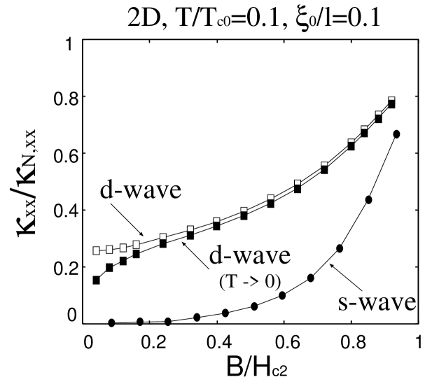
Figure 3: Magnetic-field dependences of the longitudinal thermal conductivity $\kappa_{xx}(B)$ in $s$-wave (filled circles) and $d$-wave (open squares) superconductors. $\kappa_{{\rm N},xx}=\frac{1}{3}\pi^{2}v_{\rm F}^{2}T\tau$ is the thermal conductivity in the normal state. Filled squares represent the zero-temperature value of $\kappa_{xx}(B)$ [see eq. (17)] in a $d$-wave superconductor.

Next, we show our numerical result for the thermal conductivity $\kappa_{xx}(B)$. Figure 3 shows the magnetic-field dependences of the calculated thermal conductivities in $s$-wave and $d$-wave superconductors. In the figure, we can observe a considerable difference in their field dependences: in an $s$-wave superconductor, $\kappa_{xx}(B)$ at low fields is exponentially small, while in a $d$-wave superconductor, there is a finite amount of thermal transport even at low fields. This means that the field dependence of $\kappa_{xx}(B)$ can be used as a method of probing gap nodes. However, we would like to emphasize here that unless we discuss the zero-temperature limit, $\kappa_{xx}(B)$ in both superconductors have similar field dependences. This is evident when we look at the data in Fig. 3 at finite temperatures. Actually, it is difficult to distinguish $\kappa_{xx}(B)$ in a $d$-wave superconductor from that in an $s$-wave superconductor except for their residual values, although the data are plotted in a moderately low temperature region ($T/T_{c0}=0.1$). Therefore, if we aim to use $\kappa_{xx}(B)$ to detect gap nodes, we have to extract its value at zero temperature.

Figure 4: Magnetic-field dependence of zero-temperature thermal conductivity in a $d$-wave superconductor in the unitarity limit.

In some unconventional superconductors, thermal conductivity measurements in zero magnetic field suggest the necessity of including the resonant impurity scattering in the unitarity limit. [52, 53, 54] This effect can be taken into account by performing the replacement $\frac{1}{2\tau}\langle g_{0}\rangle\to\frac{1}{2\tau}\langle g_{0}\rangle^{-1}$ in eqs. (13) and (15). Figure 4 shows the magnetic-field dependence of zero-temperature thermal conductivity in a $d$-wave superconductor with the unitarity-limit scattering. The result suggests that the magnetic-field dependence of $\kappa_{xx}(B)$ in the unitarity limit is slightly different from that in the Born limit, particularly at low fields, while the main conclusion of the previous paragraph remains unchanged.

Here, we comment on the difference between the present result and that of the BPT approximation. In the BPT approximation, the spatial average is performed incoherently as noted above using eq. (30). This procedure is expected to overestimate the vortex-core scattering and reduce the thermal conductivity. Actually, if we compare Fig. 1 of ref. Vekhter with the present result, we can see that $\kappa_{xx}(B)$ obtained by the BPT approximation is slightly suppressed to a lower value. It has weak field dependences in the intermediate fields, and shows a steep increase near $H_{c2}$. In the present study, in contrast, we do not use such an artificial spatial averaging procedure, and we take account of the spatial dependence of Green’s function in both static and linear-response equations.

A careful reader may think that the inclusion of Fermi surface anisotropy may strongly affect the result. Indeed, we have realized that an in-plane Fermi surface anisotropy does affect the field-angle-dependent specific heat and magnetization oscillations. [11, 12] To consider this possibility, we investigate the effect of in-plane Fermi surface anisotropy on the magnetic-field dependence of $\kappa_{xx}(B)$. Let us consider a model dispersion,

$$\epsilon_{\mib{p}}=\frac{1}{2m}(p_{x}^{2}+p_{y}^{2})\big{(}1+b\cos(4\varphi)\big{)},$$ (33)

where $\varphi$ denotes the azimuthal angle of Fermi momentum $\mib{p}$, and the parameter $b$ represents the degree of in-plane Fermi surface anisotropy with a fourfold symmetry. Here, we consider a case where the superconducting gap is an isotropic $s$-wave-type but the Fermi surface has in-plane anisotropy.

Figure 5 shows the magnetic-field dependences of $\kappa_{xx}(B)$ for $b=0.2$. Note that the degree of anisotropy ($b=0.2$) is sufficiently strong to reverse the in-plane magnetization oscillation pattern [12] in a $d$-wave superconductor. Concerning the field dependence of $\kappa_{xx}(B)$, there is a difference between results for $b=0$ and $b=0.2$. However, the difference is quantitative, whereas the difference between $s$-wave and $d$-wave results (Fig. 3) is qualitative. This means that the superconducting gap structure influences the field dependence of $\kappa_{xx}(B)$ more strongly than the Fermi surface anisotropy.

Figure 5: Magnetic-field dependences of $\kappa_{xx}$ in an $s$-wave superconductor with an anisotropic Fermi surface. The inset shows the corresponding data for $N(\varepsilon=0)/N_{\rm F}$. The definition of the anisotropy parameter $b$ is given in eq. (33).

4 Discussion

We discuss the origin of the difference in $\kappa_{xx}(B)$ between a $d$-wave superconductor and an $s$-wave superconductor; a $d$-wave superconductor can transport a certain amount of heat even at low fields, whereas in an $s$-wave superconductor, the thermal transport is completely suppressed. For this purpose, it is convenient to employ the zero-temperature expression of eq. (31),

$$\left.\frac{\kappa_{xx}}{T}\right|_{T\to 0}=\frac{2}{3}N_{F}\big{\langle}v_{x}^{2}{\rm Re}[g_{0}^{R}]_{\rm sp}\tau^{\rm tr}_{\mib p}(\varepsilon=0)\big{\rangle}.$$ (34)

In Fig. 6, we show the magnetic-field dependence of $\langle\tau^{\rm tr}_{\mib{p}}(\varepsilon=0)\rangle$ in both superconductors. By comparing this figure with Fig. 3, we can conclude that the main difference in $\kappa_{xx}(B)$ between $s$-wave and $d$-wave superconductors results from that in the transport lifetime $\langle\tau^{\rm tr}_{\mib p}(\varepsilon=0)\rangle$.

We can explain this difference in the following way. In an $s$-wave superconductor, the Andreev scattering rate given by the second term on the right-hand side of eq. (31) increases rapidly upon decreasing the field due to the fact that it contains the small factor ${\rm Re}[g_{0}^{R}]_{\rm sp}\sim B/H_{c2}$ in the denominator. In a $d$-wave superconductor, quasiparticles moving along the antinodal direction are dominated by the same principle. However, nodal quasiparticles do not undergo the Andreev scattering mechanism since ${\rm Re}[\widetilde{\Delta}_{\mib p}f_{0}^{{\dagger}R}+\widetilde{\Delta}^{*}_{\mib p}f_{0}^{R}]_{\rm sp}$ is almost zero, and they can transport a certain amount of heat. It is this effect that yields the difference in $\kappa_{xx}(B)$ between a nodal superconductor and a fully gapped superconductor.

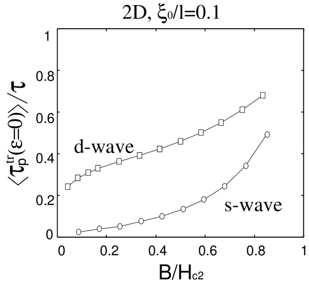
Figure 6: Magnetic-field dependence of $\langle\tau^{\rm tr}_{\mib p}(\varepsilon=0)\rangle$ in $s$-wave and $d$-wave superconductors.

This interpretation is consistent with the following physical picture provided by Boaknin et al. [55] In an $s$-wave superconductor, localized quasiparticles within vortices, which are relevant to the low-temperature properties, can give a linear-field density of states, but cannot contribute to the heat transport due to their localized nature. In a $d$-wave superconductor, on the other hand, Doppler shifted nodal quasiparticles can contribute to the heat transport, as well as to the well-known $\sqrt{B}$-dependent density of states. Thus, $\kappa_{xx}(B)$ can pick up only the contribution of extended quasiparticles. To some extent, this picture can be inferred from “extended zero-energy density of states $N_{\rm ext}(B)$” defined in ref. Nakai (see Fig. 1 therein). Our study confirmed this physical picture by a concrete numerical calculation.

In this work, we only consider a single-band superconductor with a two-dimensional Fermi surface. Hence, we do not present a detailed comparison with experiments. Instead, we discuss the implications of the present results on experiments. For $s$-wave superconductors, the present result is able to explain the following experimental observations. The magnetic-field dependence of $\kappa_{xx}(B)$ in Fig. 3 has a good correspondence to the experimental data for Nb (Fig. 3 of ref. Lowell) and V₃Si (Fig. 3(c) of ref. Boaknin2), although our result cannot be applied directly to the low-$\kappa_{\rm GL}$ superconductor Nb. Recently, Kasahara et al. also observed a similar magnetic-field dependence of $\kappa_{xx}(B)$ in a pyrochlore superconductor KOs₂O₆. [58] Concerning the $d$-wave calculation, our result is consistent with the thermal conductivity of Bi₂Sr₂CaCu₂O₈ at low fields. [59] If we limit ourselves to the low-field region, our result is also consistent with the experimental data in other (perhaps nodal) superconductors, [60, 55, 61] in that these data at low fields have stronger field dependences than the $s$-wave superconductors discussed above. On approaching the upper critical field, however, a marked difference appears. Our result shows $(H_{c2}-B)^{1/2}$ behavior near $H_{c2}$, which is consistent with the previous work, [17] while the experimental data show $(H_{c2}-B)^{\eta}$ dependences with $\eta\geq 1$. We leave this discrepancy to a future work.

5 Conclusion

In this paper, we have studied the magnetic-field dependence of the mixed-state thermal conductivity $\kappa_{xx}(B)$ in $s$-wave and $d$-wave superconductors based on the quasi-classical theory of superconductivity. The present work is valid in a wide field range from $H_{c1}$ to $H_{c2}$, and beyond the previous theoretical studies; the Doppler shift approximation is valid only near $H_{c1}$, and the Brandt-Pesch-Tewordt approximation is valid only near $H_{c2}$.

On the basis of our result, we clarified that there is indeed a clear difference in the low-temperature mixed-state thermal transport between $s$-wave and $d$-wave superconductors; in a $d$-wave superconductor, there is a finite amount of thermal transport even at low fields, while in an $s$-wave superconductor, the thermal transport is completely suppressed. This suggests that the magnetic-field dependence of $\kappa_{xx}(B)$ can be used to distinguish a nodal superconductor from a fully gapped superconductor, on the condition that we extract a suitable zero temperature-limit. Also, we microscopically confirmed the physical picture provided by Boaknin et al. [55] on the mixed-state thermal transport, and demonstrated that the above-mentioned difference in $\kappa_{xx}(B)$ mainly results from the corresponding difference in the transport lifetime.

- [1] M. Sigrist and K. Ueda: Rev. Mod. Phys. 63 (1991) 239.
- [2] C. Caroli, P. G. de Gennes, and J. Matricon: Phys. Lett. 9 (1964) 307.
- [3] G. E. Volovik: JETP Lett. 58 (1993) 469.
- [4] H. Won and K. Maki: Europhys. Lett. 30 (1995) 421.
- [5] N. B. Kopnin and G. E. Volovik: JETP Lett. 64 (1996) 690.
- [6] S. H. Simon and P. A. Lee: Phys. Rev. Lett. 78 (1997) 1548.
- [7] I. Vekhter, P. J. Hirschfeld, J. P. Carbotte, and E. J. Nicol: Phys. Rev. B 59 (1999) R9023.
- [8] M. Ichioka, A. Hasegawa, and K. Machida: Phys. Rev. B 59 (1999) 184.
- [9] N. Nakai, P. Miranović, M. Ichioka, and K. Machida: Phys. Rev. B 70 (2004) 100503(R).
- [10] P. Miranović, M. Ichioka, N. Nakai, and K. Machida: Phys. Rev. B 68 (2003) 052501.
- [11] P. Miranović, M. Ichioka, N. Nakai, and K. Machida: J. Phys.: Condens. Matter 17 (2005) 7971.
- [12] H. Adachi, P. Miranović, M. Ichioka, and K. Machida: Phys. Rev. Lett. 94 (2005) 067007.
- [13] H. Adachi, P. Miranović, M. Ichioka, and K. Machida: J. Phys. Soc. Jpn. 75 (2006) 084716.
- [14] For a review, see Y. Matsuda, K. Izawa, and I. Vekhter: J. Phys.: Condens. Matter 18 (2006) R705-R752.
- [15] A. F. Andreev: Zh. Eksp. Teor. Fiz. 46 (1964) 1823 [Sov. Phys. JETP 19 (1964) 1228].
- [16] K. Maki and T. Tsuneto: Prog. Theor. Phys. 27 (1962) 228.
- [17] K. Maki: Phys. Rev. 158 (1967) 397.
- [18] R. M. Cleary: Phys. Rev. B 1 (1970) 169.
- [19] A. Houghton and K. Maki: Phys. Rev. B 4 (1971) 843.
- [20] F. Yu, M. B. Salamon, A. J. Leggett, W. C. Lee, and D. M. Ginsberg: Phys. Rev. Lett. 74 (1995) 5136.
- [21] M. Franz: Phys. Rev. Lett. 82 (1999) 1760.
- [22] C. Kübert and P. J. Hirschfeld: Phys. Rev. Lett. 80 (1998) 4963.
- [23] Yu. S. Barash and A. A. Svidzinsky: Phys. Rev. B 58 (1998) 6476.
- [24] H. Won and K. Maki: cond-mat/0004105.
- [25] I. Vekhter and A. Houghton: Phys. Rev. Lett. 83 (1999) 4626 (see Fig. 1 therein for comparison).
- [26] M. Takigawa, M. Ichioka, and K. Machida: Eur. Phys. J. B 27 (2002) 303.
- [27] S. Dukan, T. P. Powell, and Z. Tesanović: Phys. Rev. B 66 (2002) 014517.
- [28] A. C. Durst, A. Vishwanath, and P. A. Lee: Phys. Rev. Lett. 90 (2003) 187002.
- [29] U. Brandt, W. Pesch, and L. Tewordt: Z. Phys. 201 (1967) 209.
- [30] W. Pesch: Z. Phys. B 21 (1975) 263.
- [31] H. F. Hess, R. B. Robinson, R. C. Dynes, J. M. Valles, Jr., and J. V. Waszczak: Phys. Rev. Lett. 62 (1989) 214.
- [32] G. Eilenberger: Z. Phys. 214 (1968) 195.
- [33] A. I. Larkin and Yu. N. Ovchinnikov: Zh. Eksp. Teor. Fiz. 55 (1968) 2262 [Sov. Phys.-JETP 28 (1969) 1200].
- [34] R. Kubo, M. Yokota, and S. Nakajima: J. Phys. Soc. Jpn. 12 (1957) 1203.
- [35] R. Klimesch and W. Pesch: J. Low. Temp. Phys. 32 (1978) 869.
- [36] In the Meissner state (), a Ward identity ensures that the impurity vertex corrections vanish for even-parity superconductors. [37, 38]
- [37] V. Ambegaokar and L. Tewordt: Phys. Rev. 134 (1964) A805.
- [38] P. J. Hirschfeld, P. Wölfle, and D. Einzel: Phys. Rev. B 37 (1988) 83.
- [39] M. Eschrig, J. A. Sauls, and D. Rainer: Phys. Rev. B 60 (1999) 10447.
- [40] P. Miranović: unpublished.
- [41] G. M. Eliashberg: Zh. Eksp. Teor. Fiz. 61 (1971) 1254 [Sov. Phys. JETP 34 (1972) 668].
- [42] K. Scharnberg: J. Low. Temp. Phys. 6 (1972) 51.
- [43] A. I. Larkin and Yu. N. Ovchinnikov: J. Low. Temp. Phys. 10 (1973) 407.
- [44] Yu. N. Ovchinnikov: Zh. Eksp. Teor. Fiz. 66 (1974) 1100 [Sov. Phys. JETP 39 (1974) 538].
- [45] N. Schopohl and K. Maki: Phys. Rev. B 52 (1995) 490.
- [46] N. Schopohl: cond-mat/9804064.
- [47] P. Miranović, M. Ichioka, and K. Machida: Phys. Rev. B 70 (2004) 104510.
- [48] P. W. Anderson: J. Phys. Chem. Solids 11 (1959) 26.
- [49] P. Miranović and K. Machida: Phys. Rev. B 67 (2003) 092506.
- [50] L. Tewordt and D. Fay: Phys. Rev. B 64 (2001) 024528.
- [51] H. Kusunose, T. M. Rice, and M. Sigrist: Phys. Rev. B 66 (2002) 214503.
- [52] C. J. Pethick and D. Pines: Phys. Rev. Lett. 57 (1986) 118.
- [53] P. J. Hirschfeld, D. Vollhardt, and P. Wölfle: Solid State Commun. 59 (1986) 111.
- [54] S. Schmitt-Rink, K. Miyake, and C. M. Varma: Phys. Rev. Lett. 57 (1986) 2575.
- [55] E. Boaknin, R. W. Hill, C. Proust, C. Lupien, L. Taillefer, and P. C. Canfield: Phys. Rev. Lett. 87 (2001) 237001.
- [56] J. Lowell and J. B. Sousa: J. Low. Temp. Phys. 3 (1970) 65.
- [57] E. Boaknin, M. A. Tanatar, J. Paglione, D. Hawthorn, F. Ronning, R. W. Hill, M. Sutherland, L. Taillefer, J. Sonier, S. M. Hayden, and J. W. Brill: Phys. Rev. Lett. 90 (2003) 117003.
- [58] Y. Kasahara, Y. Shimono, T. Shibauchi, Y. Matsuda, S. Yonezawa, Y. Muraoka, and Z. Hiroi: Phys. Rev. Lett. 96 (2006) 247004.
- [59] H. Aubin, K. Behnia, S. Ooi, and T. Tamegai: Phys. Rev. Lett. 82 (1999) 624.
- [60] H. Suderow, J. P. Brison, A. Huxley, and J. Flouquet: Phys. Rev. Lett. 80 (1998) 165.
- [61] K. Izawa, Y. Nakajima, J. Goryo, Y. Matsuda, S. Osaki, H. Sugawara, H. Sato, P. Thalmeier, and K. Maki: Phys. Rev. Lett. 90 (2003) 117001.