Condensed Matter Physics With Light And Atoms:
Strongly Correlated Cold Fermions in Optical Lattices.

Abstract

Various topics at the interface between condensed matter physics and the physics of ultra-cold fermionic atoms in optical lattices are discussed. The lectures start with basic considerations on energy scales, and on the regimes in which a description by an effective Hubbard model is valid. Qualitative ideas about the Mott transition are then presented, both for bosons and fermions, as well as mean-field theories of this phenomenon. Antiferromagnetism of the fermionic Hubbard model at half-filling is briefly reviewed. The possibility that interaction effects facilitate adiabatic cooling is discussed, and the importance of using entropy as a thermometer is emphasized. Geometrical frustration of the lattice, by suppressing spin long-range order, helps revealing genuine Mott physics and exploring unconventional quantum magnetism. The importance of measurement techniques to probe quasiparticle excitations in cold fermionic systems is emphasized, and a recent proposal based on stimulated Raman scattering briefly reviewed. The unconventional nature of these excitations in cuprate superconductors is emphasized.

1 Introduction: a novel condensed matter physics.

The remarkable recent advances in handling ultra-cold atomic gases have given birth to a new field: condensed matter physics with light and atoms. Artificial solids with unprecedented degree of controllability can be realized by trapping bosonic or fermionic atoms in the periodic potential created by interfering laser beams (for a recent review, see Ref. [5], and other lectures in this volume).

Key issues in the physics of strongly correlated quantum systems can be addressed from a new perspective in this context. The observation of the Mott transition of bosons in optical lattices [18, 23] and of the superfluidity of fermionic gases (see e.g. [19, 26, 52, 6]) have been important milestones in this respect, as well as the recent imaging of Fermi surfaces [27].

To quote just a few of the many promising roads for research with ultra-cold fermionic atoms in optical lattices, I would emphasize:

• the possibility of studying and hopefully understanding better some outstanding open problems of condensed matter physics, particularly in strongly correlated regimes, such as high-temperature superconductivity and its interplay with Mott localization.

• the possibility of studying these systems in regimes which are not usually reachable in condensed matter physics (e.g under time-dependent perturbations bringing the system out of equilibrium), and to do this within a highly controllable and clean setting

• the possibility of “engineering” the many-body wave function of large quantum systems by manipulating atoms individually or globally

The present lecture notes certainly do not aim at covering all these topics ! Rather, they represent an idiosyncratic choice reflecting the interests of the author. Hopefully, they will contribute in a positive manner to the rapidly developing dialogue between condensed matter physics and the physics of ultra-cold atoms. Finally, a warning and an apology: these are lecture notes and not a review article. Even though I do quote some of the original work I refer to, I have certainly omitted important relevant references, for which I apologize in advance.

2 Considerations on energy scales.

In the context of optical lattices, it is convenient to express energies in units of the recoil energy:

$$E_{R}=\frac{\hbar^{2}k_{L}^{2}}{2m}$$

in which $k_{L}=2\pi/\lambda_{L}$ is the wavevector of the laser and $m$ the mass of the atoms. This is typically of the order of a few micro-Kelvins (for a YAG laser with $\lambda_{L}=1.06\mu\rm{m}$ and ⁶Li atoms, $E_{R}\simeq 1.4\mu\rm{K}$). When venturing in the cold atoms community, condensed matter physicists who usually express energy scales in Kelvins (or electron-Volts…!) will need to remember that, in units of frequency:

$$1\,\mu\rm{K}\,\simeq\,20.8\,\rm{kHz}$$

The natural scale for the kinetic energy (and Fermi energy) of atoms in the optical lattice is not the recoil energy however, but rather the bandwidth $W$ of the Bloch band under consideration, which strongly depends on the laser intensity $V_{0}$. For a weak intensity $V_{0}\ll E_{R}$, the bandwidth $W$ of the lowest Bloch band in the optical lattice is of order $E_{R}$ itself (the free space parabolic dispersion $\hbar^{2}k^{2}/2m$ reaches the boundary of the first Brillouin zone at $k=\pi/d=k_{L}$ with $d=\lambda_{L}/2$ the lattice spacing, so that $W\simeq E_{R}$ for small $V_{0}/E_{R}$). In contrast, for strong laser intensities, the bandwidth can be much smaller than the recoil energy (Fig. 1). This is because in this limit the motion of atoms in the lattice corresponds to tunneling between two neighboring potential wells (lattice sites), and the hopping amplitude  $\rm{t}$ has the typical exponential dependence of a tunnel process. Specifically, for a simple separable potential in $D$ (=$1,2,3$) dimensions:

$$V(\mathbf{r})=V_{0}\,\sum_{i=1}^{D}\sin^{2}k_{L}r_{i}$$ (1)

one has [51]:

$$\rm{t}/E_{R}=4\pi^{-1/2}(V_{0}/E_{R})^{3/4}\,e^{-2(V_{0}/E_{R})^{1/2}}\,\,\,,\,\,\,V_{0}\gg E_{R}$$ (2)

The dispersion of the lowest band is well approximated by a simple tight-binding expression in this limit:

$$\varepsilon_{\mathbf{k}}=-2\rm{t}\sum_{i=1}^{D}\cos k_{i}$$ (3)

corresponding to a bandwidth $W=4D\rm{t}\ll E_{R}$. The dependence of the bandwidth, and of the gap between the first two bands, on $V_{0}/E_{R}$ are displayed on Fig. 1.

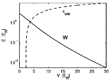
Figure 1: Width of the lowest Bloch band and gap between the first two bands for a 3-dimensional potential, as a function of laser intensity (in units of $E_{R}$) (adapted from Ref. [4]). Note that in 3 dimensions, the two lowest bands overlap for a weak lattice potential, and become separated only for $V_{0}\gtrsim 2.3E_{R}$.

Since $W$ is much smaller than $E_{R}$ for deep lattices, one may worry that cooling the gas into the degenerate regime might become very difficult. For non-interacting atoms, this indeed requires $T\ll\varepsilon_{F}$, with $\varepsilon_{F}$ the Fermi energy (energy of the highest occupied state), with $\varepsilon_{F}\leq W$ for densities such that only the lowest band is partially occupied. Adiabatic cooling may however come to the rescue when the lattice is gradually turned on [4]. This can be understood from a very simple argument, observing that the entropy of a non-interacting Fermi gas in the degenerate regime is limited by the Pauli principle to have a linear dependence on temperature:

$$S\,\propto T\,D(\varepsilon_{F})$$

where $D(\varepsilon)$ is the density of states. Hence, $TD(\varepsilon_{F})$ is expected to be conserved along constant entropy trajectories. $D(\varepsilon_{F})$ is inversely proportional to the bandwidth $W$ (with a proportionality factor depending on the density, or band filling): the density of states is enhanced considerably as the band shrinks since the one-particle states all fit in a smaller and smaller energy window. Thus, $T/W$ is expected to be essentially constant as the lattice is adiabatically turned on: the degree of degeneracy is preserved and adiabatic cooling is expected to take place. For more details on this issue, see Ref. [4] in which it is also shown that when the second band is populated, heating can take place when the lattice is turned on (because of the increase of the inter-band gap, cf. Fig. 1). For other ideas about cooling and heating effects upon turning on the lattice, see also Ref. [22]. Interactions can significantly modify these effects, and lead to additional mechanisms of adiabatic cooling, as discussed later in these notes (Sec. 6).

Finally, it is important to note that, in a strongly correlated system, characteristic energy scales are in general strongly modified by interaction effects in comparison to their bare, non-interacting values. The effective mass of quasiparticle excitations, for example, can become very large due to strong interaction effects, and correspondingly the scale associated with kinetic energy may become very small. This will also be the scale below which coherent quasiparticle excitations exist, and hence the effective scale for Fermi degeneracy. Interaction effects may also help in adiabatically cooling the system however, as discussed later in these notes.

3 When do we have a Hubbard model ?

I do not intend to review here in details the basic principles behind the trapping and manipulation of cold atoms in optical lattices. Other lectures at this school are covering this, and there are also excellent reviews on the subject, see e.g Refs. [5, 24, 51]. I will instead only summarize the basic principles behind the derivation of the effective hamiltonian. The focus of this section will be to emphasize that there are some limits on the range of parameters in which the effective hamiltonian takes the simple single-band Hubbard form [49, 48].

I consider two-component fermions (e.g two hyperfine states of identical atomic species). The hamiltonian consists in a one-body term and an interaction term:

$$H=H_{0}+H_{\rm{int}}$$ (4)

Let me first discuss the one-body part, which involves the lattice potential $V_{L}(\mathbf{r})$ as well as the potential of the trap (or of the Gaussian waist of the laser) $V_{T}(\mathbf{r})$:

$$H_{0}=\sum_{\sigma}\int d\mathbf{r}\,\psi_{\sigma}^{\dagger}(\mathbf{r})\left[-\frac{\hbar^{2}\nabla^{2}}{2m}+V_{L}(\mathbf{r})+V_{T}(\mathbf{r})\right]\psi_{\sigma}(\mathbf{r})\equiv H_{0L}+H_{0T}$$ (5)

The trapping potential having a shallow curvature as compared to the lattice spacing, the standard procedure consists in finding first the Bloch states of the periodic potential (e.g treating afterwards the trap in the local density approximation). The Bloch functions $\phi_{\mathbf{k}\nu}(\mathbf{r})$ (with $\nu$ an index labelling the band) satisfy:

$$H_{0L}|\phi_{\mathbf{k}\nu}\rangle=\varepsilon_{\mathbf{k}\nu}|\phi_{\mathbf{k}\nu}\rangle$$ (6)

with $\phi_{\mathbf{k}\nu}(\mathbf{r})=e^{i\mathbf{k}\cdot\mathbf{r}}u_{\mathbf{k}\nu}(\mathbf{r})$ and $u_{\mathbf{k}\nu}$ a function having the periodicity of the lattice. From the Bloch functions, one can construct Wannier functions $w_{\mathbf{R}\nu}(\mathbf{r})=w_{\nu}(\mathbf{r}-\mathbf{R})$, which are localized around a specific lattice site $\mathbf{R}$:

$$w_{\mathbf{R}\nu}(\mathbf{r})=w_{\nu}(\mathbf{r}-\mathbf{R})=\sum_{\mathbf{k}}e^{-i\mathbf{k}\cdot\mathbf{R}}\,\phi_{\mathbf{k}\nu}(\mathbf{r})=\sum_{\mathbf{k}}e^{i\mathbf{k}\cdot(\mathbf{r}-\mathbf{R})}\,u_{\mathbf{k}\nu}(\mathbf{r})$$ (7)

In Fig. 2, I display a contour plot of the Wannier function corresponding to the lowest band of the 2-dimensional potential (1). The characteristic spatial extension of the Wannier function associated with the lowest band is $l_{1}\sim d$ (the lattice spacing itself) for a weak potential $V_{0}\ll E_{R}$, while $l_{1}/d\sim(E_{R}/V_{0})^{1/4}\ll 1$ for a deep lattice $V_{0}\gg E_{R}$. The latter estimate is simply the extent of the ground-state wave-function of the harmonic oscillator in the quadratic well approximating the bottom of the potential.

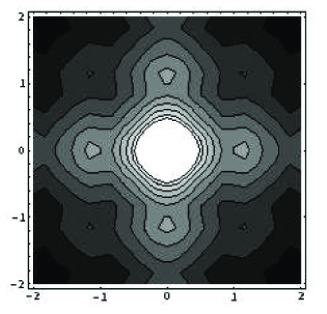
Figure 2: Contour plot of the Wannier function corresponding to the lowest band in the two-dimensional separable potential (1) with $V_{0}/E_{R}=10$. The function has the symmetry of the square lattice, and has secondary maxima on nearest-neighbor sites. The intensity of these secondary maxima control the hopping amplitude. From Ref [48].

The fermion field operator can be decomposed on the localised Wannier functions basis set, or alternatively on the Bloch functions as follows:

$$\psi^{\dagger}_{\sigma}(\mathbf{r})=\sum_{\mathbf{R}\nu}w^{*}_{\nu}(\mathbf{r}-\mathbf{R})\,c^{\dagger}_{\mathbf{R}\nu\sigma}=\sum_{\mathbf{k}\nu}\phi_{\mathbf{k}\nu}^{*}(\mathbf{r})\,c^{\dagger}_{\mathbf{k}\nu\sigma}$$ (8)

This leads to the following expression for the lattice part of the one-particle hamiltonian:

$$H_{0L}=\sum_{\mathbf{k}\nu\sigma}\varepsilon_{\mathbf{k}\nu}c^{\dagger}_{\mathbf{k}\nu\sigma}c_{\mathbf{k}\nu\sigma}=-\sum_{\mathbf{R}\mathbf{R}^{\prime}}\sum_{\nu\sigma}\rm{t}^{(\nu)}_{\mathbf{R}\mathbf{R}^{\prime}}c^{\dagger}_{\mathbf{R}\nu\sigma}c_{\mathbf{R}^{\prime}\nu\sigma}+\sum_{\mathbf{R}\nu\sigma}\varepsilon_{\nu 0}\,c^{\dagger}_{\mathbf{R}\nu\sigma}c_{\mathbf{R}\nu\sigma}$$ (9)

with the hopping parameters and on-site energies given by:

$$\rm{t}^{(\nu)}_{\mathbf{R}\mathbf{R}^{\prime}}=-\sum_{\mathbf{k}}e^{i\mathbf{k}\cdot(\mathbf{R}-\mathbf{R}^{\prime})}\,\varepsilon_{\mathbf{k}\nu}=-\int d\mathbf{r}\,w_{\nu}^{*}(\mathbf{r}-\mathbf{R})\,\left[-\frac{\hbar^{2}\nabla^{2}}{2m}+V_{L}(\mathbf{r})\right]\,w_{\nu}(\mathbf{r}-\mathbf{R}^{\prime})$$ (10)

$$\varepsilon_{\nu 0}=\sum_{\mathbf{k}}\varepsilon_{\mathbf{k}\nu}$$ (11)

Because the Bloch functions diagonalize the one-body hamiltonian, there are no inter-band hopping terms in the Wannier representation considered here. Furthermore, for a separable potential such as (1), close examination of (10) show that the oppings are only along the principal axis of the lattice: the hopping amplitudes along diagonals vanish for a separable potential (see also Sec. 7).

Let us now turn to the interaction hamiltonian. The inter-particle distance and lattice spacing are generally much larger than the hard-core radius of the inter-atomic potential. Hence, the details of the potential at short distance do not matter. Long distance properties of the potential are characterized by the scattering length $a_{s}$. As is well known, and described elsewhere in these lectures, $a_{s}$ can be tuned over a wide range of positive or negative values by varying the magnetic field close to a Feshbach resonance. Provided the extent of the Wannier function is larger than the scattering length ($l_{1}\gg a_{s}$), the following pseudopotential can be used:

$$V^{\sigma,-\sigma}_{\rm{int}}(\mathbf{r}-\mathbf{r}^{\prime})=g\,\delta(\mathbf{r}-\mathbf{r}^{\prime})\,\,\,,\,\,\,g\equiv\frac{4\pi\hbar^{2}a_{s}}{m}$$ (12)

The interaction hamiltonian then reads:

$$H_{\rm{int}}=g\,\int d\mathbf{r}\,\psi^{\dagger}_{\uparrow}(\mathbf{r})\psi_{\uparrow}(\mathbf{r})\psi^{\dagger}_{\downarrow}(\mathbf{r})\psi_{\downarrow}(\mathbf{r})$$ (13)

which can be written in the basis set of Wannier functions (assumed for simplicity to be real) as follows:

$$H_{\rm{int}}=\sum_{\mathbf{R}_{1}\mathbf{R}_{2}\mathbf{R}_{3}\mathbf{R}_{4}}\sum_{\nu_{1}\nu_{2}\nu_{3}\nu_{4}}\,U_{\mathbf{R}_{1}\mathbf{R}_{2}\mathbf{R}_{3}\mathbf{R}_{4}}^{\nu_{1}\nu_{2}\nu_{3}\nu_{4}}\,c^{\dagger}_{\mathbf{R}_{1}\nu_{1}\uparrow}c_{\mathbf{R}_{2}\nu_{2}\uparrow}c^{\dagger}_{\mathbf{R}_{3}\nu_{3}\downarrow}c_{\mathbf{R}_{4}\nu_{4}\downarrow}$$ (14)

with:

$$U_{\mathbf{R}_{1}\mathbf{R}_{2}\mathbf{R}_{3}\mathbf{R}_{4}}^{\nu_{1}\nu_{2}\nu_{3}\nu_{4}}\,=g\,\int d\mathbf{r}\,w_{\nu_{1}}(\mathbf{r}-\mathbf{R}_{1})w_{\nu_{2}}(\mathbf{r}-\mathbf{R}_{2})w_{\nu_{3}}(\mathbf{r}-\mathbf{R}_{3})w_{\nu_{4}}(\mathbf{r}-\mathbf{R}_{4})$$ (15)

The largest interaction term corresponds to two atoms on the same lattice site. Furthermore, for a deep enough lattice, with less than two atoms per site on average, the second band is well separated from the lowest one. Nelecting all other bands, and all interaction terms except the largest on-site one, one obtains the single-band Hubbard model with a local interaction term:

$$H_{H}\,=\,-\sum_{\mathbf{R}\mathbf{R}^{\prime}\sigma}\rm{t}_{\mathbf{R}\mathbf{R}^{\prime}}c^{\dagger}_{\mathbf{R}\sigma}c_{\mathbf{R}^{\prime}\sigma}+U\sum_{\mathbf{R}}\hat{n}_{\mathbf{R}\uparrow}\hat{n}_{\mathbf{R}\downarrow}$$ (16)

with:

$$U\,=\,g\,\int d\mathbf{r}\,w_{1}(\mathbf{r})^{4}$$ (17)

For a deep lattice, using the above estimate of the extension $l_{1}$ of the Wannier function of the lowest band, this leads to [51] (compare to the hopping amplitude (2) which decays exponentially):

$$\frac{U}{E_{R}}\,\simeq\,\sqrt{\frac{8}{\pi}}\,a_{s}k_{L}\,\left(\frac{V_{0}}{E_{R}}\right)^{3/4}$$ (18)

The hopping amplitude and on-site interaction strength $U$, calculated for the lowest band of a three-dimensional separable potential, are plotted as a function of $V_{0}/E_{R}$ in Fig. 3.

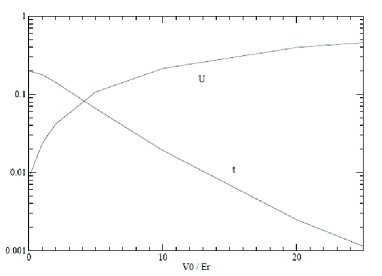
Figure 3: Hopping amplitude $\rm{t}$ and on-site interaction energy $U$, as a function of $V_{0}/E_{R}$, for the three-dimensional separable potential (1) corresponding to a cubic lattice. $\rm{t}$ is expressed in units of $E_{R}$ and $U$ in units of $100\,E_{R}\,a_{s}/d$, with $a_{s}$ the scattering length and $d$ the lattice spacing. From Ref [48].

Let us finally discuss the conditions under which this derivation of a simple single-band Hubbard model is indeed valid. We have made 3 assumptions: i) neglect the second band, ii) neglect other interactions besides the Hubbard $U$ and iii) replace the actual interatomic potential by the pseudopotential approximation. Assumption i) is justified provided the second band is not populated (less than two fermions per site, and $V_{0}$ not too small so that the two bands do not overlap, i.e $V_{0}\gg 2.3E_{R}$ cf. Fig. 1), but also provided the energy cost for adding a second atom on a given lattice site which already has one is indeed set by the interaction energy. If $U$ as given by (17) becomes larger than the separation $\Delta=\sum_{\mathbf{k}}(\varepsilon_{\mathbf{k}2}-\varepsilon_{\mathbf{k}1})$ between the first two bands, then it is more favorable to add the second atom in the second band (which then cannot be neglected, even if not populated). Hence one must have $U<\Delta$. For the pseudopotential to be valid (assumption -iii), the typical distance between two atoms in a lattice well (which is given by the extension of the Wannier function $l_{1}$) must be larger than the scattering length: $l_{1}\gg a_{s}$. Amusingly, for deep lattices, this actually coincides with the requirement $U\ll\Delta$ and boils down to (at large $V_{0}/E_{R}$):

$$\frac{a_{s}}{d}\,\lesssim\,\left(\frac{V_{0}}{E_{R}}\right)^{-1/4}$$ (19)

In order to see this, one simply has to use the above estimates of $l_{1}$ ($\sim d(E_{R}/V_{0})^{1/4}$) and $U/E_{R}$ ($\sim a_{s}/d(V_{0}/E_{R})^{3/4}$) and that of the separation $\Delta\simeq(E_{R}V_{0})^{1/2}$ in this limit. Eq. (19) actually shows that for a deep lattice, the scattering length should not be increased too much if one wants to keep a Hubbard model with an interaction set by the scattering length itself and given by (18). For larger values of $a_{s}$, it may be that a one-band Hubbard description still applies (see however below for the possible appearance of new interaction terms), but with an effective $U$ given by the inter-band separation $\Delta$ rather than set by $a_{s}$. This requires a more precise investigation of the specific case at hand .

Finally, the possible existence of other interaction terms besides the on-site $U$ (-ii), and when they can be neglected, requires a more careful examination. These interactions must be smaller than $U$ but also than the hopping $\rm{t}$ which we have kept in the hamiltonian. In Ref. [49, 48], we considered this in more details and concluded that the most ‘dangerous’ coupling turns out to be a kind of ‘density-assisted’ hopping between two nearest-neighbor sites, of the form:

$$V_{h}\sum_{\langle\mathbf{R}\mathbf{R}^{\prime}\rangle}\sum_{\sigma}\,\hat{n}_{\mathbf{R},-\sigma}c^{\dagger}_{\mathbf{R}\sigma}c_{\mathbf{R}^{\prime},\sigma}+\rm{h.c}$$ (20)

with:

$$V_{h}=g\,\int d\mathbf{r}\,w_{1}(\mathbf{r})^{3}w_{1}(\mathbf{r}+\mathbf{d})=g\,\left(\int dxw_{x}(x)^{3}w_{x}(x+d)\right)\left(\int dyw_{y}(y)^{4}\right)\left(\int dzw_{z}(z)^{4}\right)$$

where $\mathbf{d}$ denotes a lattice translation between nearest-neighbor sites, and the last formula holds for a separable potential. The validity of the single-band Hubbard model also requires that $V_{h}\ll\rm{t},U$. All these requirements insuring that a simple Hubbard model description is valid are summarized on Fig. 4.

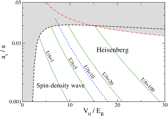
Figure 4: Range of validity of the simple one-band Hubbard model description, for a separable three-dimensional potential (1), as a function of lattice depth (normalized to recoil energy) $V_{0}/E_{R}$, and scattering length (normalized to lattice spacing) $a_{s}/d$. In the shaded region, the one-band Hubbard description is questionable. The dashed line corresponds to the condition $U/\Delta=0.1$, with $\Delta$ the gap to the second band: above this line, other bands may have to be taken into account and the pseudopotential approximation fails, so that $U$ is no longer given by (17). The dashed-dotted line corresponds to $V_{h}/\rm{t}=0.1$: above this line, $V_{h}$ becomes sizeable. These conditions may be somewhat too restrictive, but are meant to emphasize the points raised in the text. Also indicated on the figure are: contour plots of the values of the Hubbard coupling $U/\rm{t}$, and the regions corresponding to the spin-density wave and Heisenberg regimes of the antiferromagnetic ground-state at half-filling (Sec.5). The crossover between these regimes is indicated by the dotted line ($U/t=10$), where $T_{N}/t$ is maximum. Figure from Ref. [49].

4 The Mott phenomenon.

Strong correlation effects appear when atoms “hesitate” between localized and itinerant behaviour. In such a circumstance, one of the key difficulties is to describe consistently an entity which is behaving simultaneously in a wave-like (delocalized) and particle-like (localized) manner. Viewed from this perspective, strongly correlated quantum systems raise questions which are at the heart of the quantum mechanical world.

The most dramatic example is the possibility of a phase transition between two states: one in which atoms behave in an itinerant manner, and one in which they are localized by the strong on-site repulsion in the potential wells of a deep lattice. In the Mott insulating case, the energy gain which could be obtained by tunneling between lattice sites ($\sim D\rm{t}\simeq W$) becomes unfavorable in comparison to the cost of creating doubly occupied lattice sites ($\sim U$). This cost will have to be paid for sure if there is, for example, one atom per lattice site on average. This is the famous Mott transition. The proximity of a Mott insulating phase is in fact responsible for many of the intriguing properties of strongly correlated electron materials in condensed matter physics, as illustrated below in more details. This is why the theoretical proposal [23] and experimental observation [18] of the Mott transition in a gas of ultra-cold bosonic atoms in an optical lattice have truly been pioneering works establishing a bridge between modern issues in condensed matter physics and ultra-cold atomic systems.

4.1 Mean-field theory of the bosonic Hubbard model

Even though this school is devoted to fermions, I find it useful to briefly describe the essentials of the mean-field theory of the Mott transition in the bosonic Hubbard model. Indeed, this allows to focus on the key phenomenon (namely, the blocking of tunneling by the on-site repulsive interaction) without having to deal with the extra complexities of fermionic statistics and spin degrees of freedom which complicate the issue in the case of fermions (see below).

Consider the Hubbard model for single-component bosonic atoms:

$$H=-\sum_{ij}\rm{t}_{ij}\,b^{\dagger}_{i}b_{j}+\frac{U}{2}\sum_{i}\hat{n}_{i}(\hat{n}_{i}-1)-\mu\sum_{i}\hat{n}_{i}$$ (21)

As usually the case in statistical mechanics, a mean-field theory can be constructed by replacing this hamiltonian on the lattice by an effective single-site problem subject to a self-consistency condition. Here, this is naturally achieved by factorizing the hopping term [13, 43]: $b^{\dagger}_{i}b_{j}\rightarrow\rm{const.}+\langle b^{\dagger}_{i}\rangle b_{j}+b^{\dagger}_{i}\langle b_{j}\rangle+\rm{fluct.}$. Another essentially equivalent formulation is based on the Gutzwiller wavefunction [41, 31]. The effective 1-site hamiltonian for site $i$ reads::

$$h_{\rm{eff}}^{(i)}=-\lambda_{i}b^{\dagger}-\lambda_{i}b+\frac{U}{2}\hat{n}(\hat{n}-1)-\mu\hat{n}$$ (22)

In this expression, $\lambda_{i}$ is a “Weiss field” which is determined self-consistently by the boson amplitude on the other sites of the lattice through the condition:

$$\lambda_{i}=\sum_{j}\rm{t}_{ij}\,\langle b_{j}\rangle$$ (23)

For nearest-neighbour hopping on a uniform lattice of connectivity $z$, with all sites being equivalent, this reads:

$$\lambda=z\,\rm{t}\,\langle b\rangle$$ (24)

These equations are easily solved numerically, by diagonalizing the effective single-site hamiltonian (22), calculating $\langle b\rangle$ and iterating the procedure such that (24) is satisfied. The boson amplitude $\langle b\rangle$ is an order-parameter which is non-zero in the superfluid phase. For densities corresponding to an integer number $n$ of bosons per site on average, one finds that $\langle b\rangle$ is non-zero only when the coupling constant $U/\rm{t}$ is smaller than a critical ratio $(U/\rm{t})_{c}$ (which depends on the filling $n$). For $U/\rm{t}>(U/\rm{t})_{c}$, $\langle b\rangle$ (and $\lambda$) vanishes, signalling the onset of a non-superfluid phase in which the bosons are localised on the lattice sites. For non-integer values of the density, the system remains a superfluid for arbitrary couplings.

It is instructive to analyze these mean-field equations close to the critical value of the coupling: because $\lambda$ is then small, it can be treated in perturbation theory in the effective hamiltonian (22). Let us start with $\lambda=0$. We then have a collection of disconnected lattice sites (i.e no effective hopping, often called the “atomic limit” in condensed matter physics). The ground-state of an isolated site is the number state $|n\rangle$ when the chemical potential is in the range $\mu\in[(n-1)U,nU]$. When $\lambda$ is small, the perturbed ground-state becomes:

$$|\psi_{0}\rangle=|n\rangle-\lambda\,\left[\frac{\sqrt{n}}{U(n-1)-\mu}|n-1\rangle+\frac{\sqrt{n+1}}{\mu-Un}|n+1\rangle\right]$$ (25)

so that:

$$\langle\psi_{0}|b|\psi_{0}\rangle=-\lambda\,\left[\frac{n}{U(n-1)-\mu}+\frac{n+1}{\mu-Un}\right]$$ (26)

Inserting this in the self-consistency condition yields:

$$\lambda=-z\,\rm{t}\,\lambda\,\left[\frac{n}{U(n-1)-\mu}+\frac{n+1}{\mu-Un}\right]+\cdots$$ (27)

where “…” denotes higher order terms in $\lambda$. As usual, the critical value of the coupling corresponds to the vanishing of the coefficient of the term linear in $\lambda$ (corresponding to the mass term of the expansion of the Landau free-energy). Hence the critical boundary for a fixed average (integer) density $n$ is given by:

$$\frac{z\rm{t}}{U}\,=\,\frac{(n-\mu/U)(\mu/U-n+1)}{1+\mu/U}$$ (28)

This expression gives the location of the critical boundary as a function of the chemical potential. In the ($\rm{t}/U,\mu/U$) plane, the phase diagram (Fig. 5) consists of lobes inside which the density is integer and the system is a Mott insulator. Outside these lobes, the system is a superfluid. The tip of a given lobe corresponds to the the maximum value of the hopping at which an insulating state can be found. For $n$ atoms per site, this is given by:

$$\frac{z\rm{t}}{U}|_{c,n}=\rm{Max}_{x\in[n-1,n]}\frac{(n-x)[x-n+1]}{1+x}=\frac{1}{2n+1+2\sqrt{n(n+1)}}$$ (29)

So that the critical interaction strength is $(U/z\rm{t})_{c}\simeq 5.8$ for $n=1$, and increases as $n$ increases ($(U/z\rm{t})_{c}\sim 4n$ for large $n$).

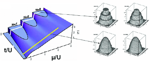
Figure 5: Left: phase diagram of the Bose Hubbard model as a function of chemical potential $\mu/U$ and coupling $\rm{t}/U$. An incompressible Mott insulator is found within each lobe of integer density. Right: density profiles in a harmonic trap. The “wedding cake” structure (see text) is due to the incompressibility of the Mott insulator (numerical calculations courtesy of H.Niemeyer and H.Monien, figure courtesy F.Gerbier).

4.2 Incompressibility of the Mott phase and “wedding-cake” structure of the density profile in the trap

The Mott insulator has a gap to density excitations and is therefore an incompressible state: adding an extra particle costs a finite amount of energy. This is clear from the mean-field calculation above: if we want to vary the average density from infinitesimally below an integer value $n$ to infinitesimally above, we have to change the chemical potential across the Mott gap:

$$\Delta_{g}(n)=\mu_{+}(n)-\mu_{-}(n)$$ (30)

where $\mu_{\pm}$ are the solutions of the quadratic equation corresponding to (28), i.e:

$$(\mu/U)^{2}-[2n-1-(z\rm{t}/U)](\mu/U)+n(n-1)+(z\rm{t}/U)=0$$ (31)

yielding:

$$\Delta_{g}(n)=U\,\left[(\frac{z\rm{t}}{U})^{2}-2(2n+1)\frac{z\rm{t}}{U}+1\right]^{1/2}$$ (32)

The Mott gap is $\sim U$ at large $U$ and vanishes at the critical coupling ($\propto\sqrt{U-U_{c}}$ within mean-field theory).

The existence of a gap means that the chemical potential can be changed within the gap without changing the density. As a result, when the system is placed in a trap, it displays density plateaus corresponding to the Mott state, leading to a “wedding cake” structure of the density profile (Fig. 5). This is easily understood in the local density approximation, in which the local chemical potential is given by: $\mu(\mathbf{r})=\bar{\mu}-m\omega_{0}^{2}r^{2}/2$, yielding a maximum extension of the plateau: $\sim(2\Delta_{g}/m\omega_{0}^{2})^{1/2}$. Several authors have studied these density plateaus beyond the LDA by numerical simulation (see e.g [2]), and they have been recently observed experimentally [15].

4.3 Fermionic Mott insulators and the Mott transition in condensed matter physics

The discussion of Mott physics in the fermionic case is somewhat complicated by the presence of the spin degrees of freedom (corresponding e.g to 2 hyperfine states in the context of cold atoms). Of course, we could consider single component fermions, but two of those cannot be put on the same lattice site because of the Pauli principle, hence spinless fermions with one atom per site on average simply form a band insulator. Mott and charge density wave physics would show up in this context when we have e.g one fermion out of two sites, but this requires inter-site (e.g dipolar) interactions.

The basic physics underlying the Mott phenomenon in the case of two-component fermions with one particle per site on average is the same as in the bosonic case however: the strong on-site repulsion overcomes the kinetic energy and makes it unfavorable for the particles to form an itinerant (metallic) state. From the point of view of band theory, we would have a metal, with one atom per unit cell and a half-filled band. Instead, at large enough values of $U/\rm{t}$, a Mott insulating state with a charge gap develops. This is purely charge physics, not spin physics.

One must however face the fact that the naive Mott insulating state has a huge spin entropy: it is a paramagnet in which the spin of the atom localized on a given site can point in either direction. This huge degeneracy must be lifted as one cools down the system into its ground-state (Nernst). How this happens will depend on the details of the model and of the residual interactions between the spin degrees of freedom. In the simplest case of a two-component model on an unfrustrated (e.g. bipartite) lattice, the spins order into an antiferromagnetic ground-state. This is easily understood in strong coupling $U\gg\rm{t}$ by Anderson’s superexchange mechanism: in a single-band model, a nearest-neighbor magnetic exchange is generated, which reads on each lattice bond:

$$J_{\rm{AF}}\,=\,\frac{4\rm{t}_{ij}^{2}}{U}$$ (33)

This expression is easily understood from second-order degenerate perturbation theory in the hopping, starting from the limit of decoupled sites ($\rm{t}=0$). Then, two given sites have a 4-fold degenerate ground-state. For small $\rm{t}$, this degeneracy is lifted: the singlet state is favoured because a high-energy virtual state is allowed in the perturbation expansion (corresponding to a doubly occupied state), while no virtual excited state is connected to the triplet state because of the Pauli principles (an atom with a given spin cannot hop to a site on which another atom with the same spin already exists). If we focus only on low-energies, much smaller than the gap to density excitations ($\sim U$ at large $U$), we can consider the reduced Hilbert space of states with exactly one particle per site. Within this low-energy Hilbert space, the Hubbard model with one particle per site on average reduces to the quantum Heisenberg model:

$$H_{J}\,=\,J_{\rm{AF}}\,\sum_{\langle ij\rangle}\,\mathbf{S}_{i}\cdot\mathbf{S}_{j}$$ (34)

Hence, there is a clear separation of scales at strong coupling: for temperatures/energies $T\lesssim U$, density fluctuations are suppressed and the physics of a paramagnetic Mott insulator (with a large spin entropy) sets in. At a much lower scale $T\lesssim J_{\rm{AF}}\,$, the residual spin interactions set in and the true ground-state of the system is eventually reached (corresponding, in the simplest case, to an ordered antiferromagnetic state).

At this point, it is instructive to pause for a moment and ask what real materials do in the condensed matter physics world. Materials with strong electronic correlations are those in which the relevant electronic orbitals (those corresponding to energies close to the Fermi energy) are quite strongly localized around the nuclei, so that a band theory description in terms of Bloch waves is not fully adequate (and may even fail completely). This happens in practice for materials containing partially filled $d$- and $f$-shells, such as transition metals, transition-metal oxides, rare earths, actinides and their compounds, as well as many organic conductors (which have small bandwidths). In all these materials, Mott physics and the proximity to a Mott insulating phase plays a key role. In certain cases, these materials are poised rather close to the localisation/delocalisation transition so that a small perturbation can tip off the balance. This is the case, for example, of a material such as V₂O₃ (vanadium sesquioxide), whose phase diagram is displayed in Fig. 6.

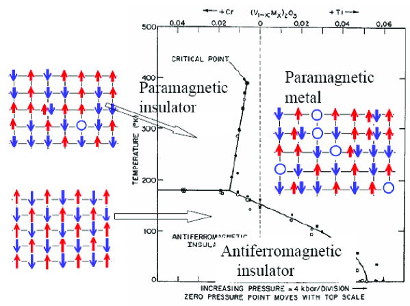
Figure 6: Phase diagram of V₂O₃ as a function of pressure of Cr-substitution, and temperature. The cartoons illustrate the nature of each phase (paramagnetic Mott insulator, paramagnetic metal, antiferromagnetic Mott insulator).

The control parameter in this material is the applied pressure (or chemical substitution by other atoms on vanadium sites), which change the unit-cell volume and hence the bandwidth (as well, in fact, as other characteristics of the electronic structure, such as the crystal-field splitting). It is seen from Fig. 6 that all three phases discussed above are realized in this material. At low pressure and high temperature, one has a paramagnetic Mott insulator with fluctuating spins. As the pressure is increased, this insulator evolves abruptly into a metallic state, through a first order transition line (which ends at a critical endpoint at $T_{c}\simeq 450$K). At low temperature $T<T_{N}\simeq 170\,$K, the paramagnetic Mott insulator orders into an antiferromagnetic Mott insulator. Note that the characteristic temperatures at which these transitions take place are considerably smaller than the bare electronic energy scales ($\sim 1$eV$\simeq 12000\,$K).

On Fig. 6, I have given for each phase a (much oversimplified) cartoon of what the phase looks like in real space. The paramagnetic Mott insulator is a superposition of essentially random spin configurations, with almost only one electron per site and very few holes and double occupancy. The antiferromagnetic insulator has Néel-like long range order (but of course the wavefunction is a complicated object, not the simple Néel classical wavefunction). The metal is the most complicated when looking at it in real space: it is a superposition of configurations with singly occupied sites, holes, and double occupancies.

Of course, such a material is far less controllable than ultra-cold atomic systems: as we apply pressure many things change in the material, not only e.g the electronic bandwidth. Also, not only the electrons are involved: increasing the lattice spacing as pressure is reduced decreases the electronic cohesion of the crystal and the ions of the lattice may want to take advantage of that to gain elastic energy: there is indeed a discontinuous change of lattice spacing through the first-order Mott transition line. Atomic substitutions introduce furthermore some disorder into the material. Hence, ultra-cold atomic systems offer an opportunity to disentangle the various phenomena and study these effects in a much more controllable setting.

4.4 (Dynamical) Mean-field theory for fermionic systems

In section. 4.1, we saw how a very simple mean-field theory of the Mott phenomenon can be constructed for bosons, by using $\langle b\rangle$ as an order parameter of the superfluid phase and making an effective field (Weiss) approximation for the inter-site hopping term. Unfortunately, this cannot be immediately extended to fermions. Indeed, we cannot give an expectation value to the single fermion operator, and $\langle c\rangle$ is not an order parameter of the metallic phase anyhow.

A generalization of the mean-field concept to many-body fermion systems does exist however, and is known as the “dynamical mean-field theory” (DMFT) approach. There are many review articles on the subject (e.g [17, 30, 16]), so I will only describe it very briefly here. The basic idea is still to replace the lattice system by a single-site problem in a self-consistent effective bath. The exchange of atoms between this single site and the effective bath is described by an amplitude, or hybridization function , $\Delta(i\omega_{n})$, which is a function of energy (or time). It is a quantum-mechanical generalization of the static Weiss field in classical statistical mechanics, and physically describes the tendancy of an atom to leave the site and wander in the rest of the lattice. In a metallic phase, we expect $\Delta(\omega)$ to be large at low-energy, while in the Mott insulator, we expect it to vanish at low-energy so that motion to other sites is blocked.

The (site+effective bath) problem is described by an effective action, which for the paramagnetic phase of the Hubbard model reads:

$$S_{\rm{eff}}=-\sum_{n}\sum_{\sigma}c^{\dagger}_{\sigma}(i\omega_{n})[i\omega_{n}+\mu-\Delta(i\omega_{n})]c_{\sigma}(i\omega_{n})+U\,\int_{0}^{\beta}d\tau\,n_{\uparrow}\,n_{\downarrow}$$ (35)

From this local effective action, a one-particle Green’s function and self-energy can be obtained as:

$$G(\tau-\tau^{\prime})=-\langle T\,c_{\sigma}(\tau)c^{\dagger}_{\sigma}(\tau^{\prime})\rangle_{\rm{eff}}$$ (36)

$$\Sigma(i\omega_{n})=i\omega_{n}+\mu-\Delta(i\omega_{n})-G(i\omega_{n})^{-1}$$ (37)

The self-consistency condition, which closes the set of dynamical mean-field theory equations, states that the Green’s function and self-energy of the (single-site+bath) problem coincides with the corresponding local (on-site) quantities in the original lattice model. This yields:

$$G(i\omega_{n})=\sum_{\mathbf{k}}\,\frac{1}{i\omega_{n}+\mu-\Sigma(i\omega_{n})-\varepsilon_{\mathbf{k}}}=\sum_{\mathbf{k}}\,\frac{1}{\Delta(i\omega_{n})+G(i\omega_{n})^{-1}-\varepsilon_{\mathbf{k}}}$$ (38)

Equations (35,38) form a set of two equations which determine self-consistently both the local Green’s function $G$ and the dynamical Weiss field $\Delta$. Numerical methods are necessary to solve these equations, since one has to calculate the Green’s function of a many-body (albeit local) problem. Fortunately, there are several computational algorithms which can be used for this purpose.

On Fig. 7, I display the schematic shape of the generic phase diagram obtained with dynamical mean-field theory, for the one band Hubbard model with one particle per site. At high temperature, there is a crossover from a Fermi liquid (metallic) state at weak coupling to a paramagnetic Mott insulator at strong coupling. Below some critical temperature $T_{c}$, this crossover turns into a first-order transition line. Note that $T_{c}$ is a very low energy scale: $T_{c}\simeq W/80$, almost two orders of magnitude smaller than the bandwidth. Whether this critical temperature associated with the Mott transition can be actually reached depends on the concrete model under consideration. In the simplest case, i.e for a single band with nearest-neighbor hopping on an unfrustrated lattice, long range antiferromagnetic spin ordering takes place already at a temperature far above $T_{c}$, as studied in more details in the next section. Hence, only a finite-temperature crossover, not a true phase transition, into a paramagnetic Mott insulator will be seen in this case. However, if antiferromagnetism becomes frustrated, the Néel temperature can be strongly suppressed, revealing genuine Mott physics, as shown in the schematic phase diagram of Fig. 7.

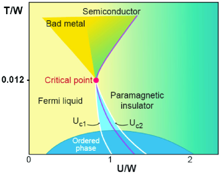
Figure 7: Schematic phase diagram of the half-filled fermionic Hubbard model, as obtained from DMFT. It is depicted here for the case of a frustrated lattice (e.g with next-nearest neighbour hopping), which reduces the transition temperature into phases with long-range spin ordering. Then, a first-order transition from a metal to a paramagnetic Mott insulator becomes apparent. For the unfrustrated case, see next section. Adapted from [29].

5 Ground-state of the 2-component Mott insulator: antiferromagnetism.

Here, I consider in more details the simplest possible case of a one-band Hubbard model, with nearest-neighbor hopping on a bipartite (e.g cubic) lattice and one atom per site on average. The phase diagram, as determined by various methods (Quantum Monte Carlo, as well as the DMFT approximation) is displayed on Fig. 8. There are only two phases: a high-temperature paramagnetic phase, and a low-temperature antiferromagnetic phase which is an insulator with a charge gap. Naturally, within the high-temperature phase, a gradual crossover from itinerant to Mott localized is observed as the coupling $U/\rm{t}$ is increased, or as the temperature is decreased below the Mott gap ($\sim U$ at large $U/\rm{t}$). Note that the mean-field estimate of the Mott critical temperature $T_{c}\simeq W/80$ is roughly a factor of two lower than that of the maximum value of the Néel temperature for this model ($\sim W/40$), so we do not expect the first-order Mott transition line and critical endpoint to be apparent in this unfrustrated situation.

Both the weak coupling and strong coupling sides of the phase diagram are rather easy to understand. At weak coupling, we can treat $U/\rm{t}$ by a Hartree-Fock decoupling, and construct a static mean-field theory of the antiferromagnetic transition. The broken symmetry into $(A,B)$ sublattices reduces the Brillouin zone to half of its original value, and two bands are formed which read:

$$E_{\mathbf{k}}^{\pm}=\pm\,\sqrt{\varepsilon_{\mathbf{k}}^{2}+\Delta_{g}^{2}/4}$$ (39)

In this expression, $\Delta$ is the Mott gap, which within this Hartree approximation is directly related to the staggered magnetization of the ground-state $m_{s}=\langle n_{A\uparrow}-n_{A\downarrow}\rangle=\langle n_{B\downarrow}-n_{B\uparrow}\rangle$ by:

$$\Delta_{g}=U\,m_{s}$$ (40)

This leads to a self-consistent equation for the gap (or staggered magnetization):

$$\frac{U}{2}\sum_{\mathbf{k}\in\rm{RBZ}}\frac{1}{\sqrt{\varepsilon_{\mathbf{k}}^{2}+\Delta_{g}^{2}/4}}=1$$ (41)

At weak-coupling, where this Hartree approximation is a reasonable starting point, the antiferromagnetic instability occurs for arbitrary small $U/\rm{t}$ and the gap, staggered magnetization and Néel temperature are all exponentially small. In this regime, the antiferromagnetism is a “spin density-wave” with wavevector $\mathbf{Q}=(\pi,\cdots,\pi)$ and a very weak modulation of the order parameter.

It should be noted that this spin-density wave mean-field theory provides a band theory (Slater) description of the insulating ground-state: because translational invariance is broken in the antiferromagnetic ground-state, the Brillouin zone is halved, and the ground-state amounts to fully occupy the lowest Hartree-Fock band. This is because there is no separation of energy scales at weak coupling: the spin and charge degrees of freedom get frozen at the same energy scale. The existence of a band-like description in the weak coupling limit is often a source of confusion, leading some people to overlook that Mott physics is primarily a charge phenomenon, as it becomes clear at intermediate and strong coupling.

In the opposite regime of strong coupling $U\gg\rm{t}$, we have already seen that the Hubbard model reduces to the Heisenberg model at low energy. In this regime, the Néel temperature is proportional to $J_{\rm{AF}}\,$, with quantum fluctuations significantly reducing $T_{N}/J_{\rm{AF}}\,$ from its mean-field value: numerical simulations [45] yield $T_{N}/J_{\rm{AF}}\,\simeq 0.957$ on the cubic lattice. Hence, $T_{N}/\rm{t}$ becomes small (as $\sim\rm{t}/U$) in strong coupling. In between these two regimes, $T_{N}$ reaches a maximum value (Fig. 8).

On Fig. 4, we have indicated the two regimes corresponding to spin-density wave and Heisenberg antiferromagnetism, in the $(V_{0}/E_{R},a_{s}/d)$ plane. In fact, the crossover between these two regimes is directly equivalent to the BCS-BEC crossover for an attractive interaction. For one particle per site, and a bipartite lattice, the Hubbard model with $U>0$ maps onto the same model with $U<0$ under the particle-hole transformation (on only one spin species):

$$c_{i\uparrow}\,\rightarrow\,\,\widetilde{c}_{i\uparrow}\,\,\,,\,\,\,c_{i\downarrow}\,\rightarrow\,(-1)^{i}\,\widetilde{c}^{\dagger}_{i\downarrow}$$ (42)

with $(-1)^{i}=+1$ on the A-sublattice and $=-1$ on the B-sublattice. The spin density wave (weak coupling) regime corresponds to the BCS one and the Heisenberg (strong-coupling) regime to the BEC one.

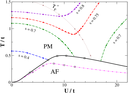
Figure 8: Phase diagram of the half-filled Hubbard model on the cubic lattice: antiferromagnetic (AF) and paramagnetic (PM) phases. Transition temperature within the DMFT approximation (plain curve, open circles) and from the QMC calculation of Ref. [45] (dot-dashed curve, squares). Dashed lines: isentropic curves (s=0.4,0.7,0.75,0.8), computed within DMFT. Dotted line: quasiparticle coherence scale $T_{F}^{*}(U)$. See Ref. [49] for more details.

6 Adiabatic cooling: entropy as a thermometer.

As discussed above, the Néel ordering temperature is a rather low scale as compared to the bandwidth. Considering the value of $T_{N}$ at maximum and taking into account the appropriate range of $V_{0}/E_{R}$ and the constraints on the Hubbard model description, one would estimate that temperatures on the scale of $\sim 10^{-2}E_{R}$ must be reached. This is at first sight a bit deceptive, and one might conclude that the prospects for cooling down to low enough temperatures to reach the antiferromagnetic Mott insulator are not so promising.

In Ref. [49] however, we have argued that one should in fact think in terms of entropy rather than temperature, and that interaction effects in the optical lattice lead to adiabatic cooling mechanisms which should help.

Consider the entropy per particle of the homogeneous half-filled Hubbard model: this is a function $s(T,U)$ of the temperature and coupling . The entropy itself is a good thermometer since it is an increasing function of temperature ($\partial s/\partial T>0$). Assuming that an adiabatic process is possible, the key point to reach the AF phase is to be able to prepare the system in a state which has a smaller entropy than the entropy at the Néel transition, i.e along the critical boundary:

$$s_{N}(U)\,\equiv\,s\left(T_{N}(U),U\right)$$ (43)

It is instructive to think of the behaviour of this quantity as a function of $U$. At weak-coupling (spin-density wave regime), $s_{N}(U)$ is expected to be exponentially small. In contrast, in the opposite Heisenberg regime at large $U/\rm{t}$, $s_{N}$ will reach a finite value $s_{H}$, which is the entropy of the quantum Heisenberg model at its critical point. $s_{H}$ is a pure number which depends only on the specific lattice of interest. Mean-field theory of the Heisenberg model yields $s_{H}=\ln 2$, but quantum fluctuations will reduce this number. In [49], this reduction was estimated to be of order $50\%$ on the cubic lattice, i.e $s_{H}\simeq\ln 2/2$, but a precise numerical calculation would certainly be welcome. How does $s_{N}$ evolve from weak to strong coupling ? A rather general argument suggests that it should go through a maximum $s_{\rm{max}}>s_{H}$. In order to see this, we take a derivative of $s_{N}(U)$ with respect to coupling, observing that:

$$\frac{\partial s}{\partial U}=-\frac{\partial p_{\,2}}{\partial T}$$ (44)

In this expression, $p_{\,2}$ is the probability that a given site is doubly occupied: $p_{\,2}\equiv\langle n_{i\uparrow}n_{i\downarrow}\rangle$. This relation stems from the relation between entropy and free-energy: $s=-\partial f/\partial T$ and $\partial f/\partial U=p_{\,2}$ Hence, one obtains:

$$\frac{ds_{N}}{dU}=\frac{c(T_{N})}{T_{N}}\,\frac{dT_{N}}{dU}-\frac{\partial p_{\,2}}{\partial T}|_{T=T_{N}}$$ (45)

in which $c(T,U)$ is the specific heat per particle: $c=T\partial s/\partial T$. If only the first term was present in the r.h.s of this equation, it would imply that $s_{N}$ is maximum exactly at the value of the coupling where $T_{N}$ is maximum (note that $c(T_{N})$ is finite ($\alpha<0$) for the 3D-Heisenberg model). Properties of the double occupancy discussed below show that the second term in the r.h.s has a similar variation than the first one. These considerations suggest that $s_{N}(U)$ does reach a maximum value $s_{\rm{max}}$ at intermediate coupling, in the same range of $U$ where $T_{N}$ reaches a maximum. Hence, $s_{N}(U)$ has the general form sketched on Fig. 9. This figure can be viewed as a phase diagram of the half-filled Hubbard model, in which entropy itself is used as a thermometer, a very natural representation when addressing adiabatic cooling. Experimentally, one may first cool down the gas (in the absence of the optical lattice) down to a temperature where the entropy per particle is lower than $s_{\rm{max}}$ (this corresponds to $T/T_{F}<s_{\rm{max}}/\pi^{2}$ for a trapped ideal gas). Then, by branching on the optical lattice adiabatically, one could increase $U/t$ until one particle per site is reached over most of the trap: this should allow to reach the antiferromagnetic phase. Assuming that the timescale for adiabaticity is simply set by the hopping, we observe that typically $\hbar/\rm{t}\sim 1\textrm{ms}$.

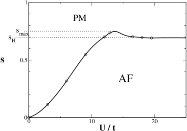
Figure 9: Schematic phase diagram of the one-band Hubbard model at half filling, as a function of entropy and coupling constant. The marked dots are from a DMFT calculation (in which case $s_{H}=\ln 2$), but the shape of the critical boundary is expected to be general (with $s_{H}<\ln 2$ reduced by quantum fluctuations).

The shape of the isentropic curves in the plane $(U/\rm{t},T/\rm{t})$, represented on Fig. 8, can also be discussed on the basis of Eq. (45). Taking a derivative of the equation defining the isentropic curves: $s(T_{i}(U),U)=\rm{const.}$, one obtains:

$$c(T_{i})\,\frac{\partial T_{i}}{\partial U}=T_{i}\,\frac{\partial p_{\,2}}{\partial T}|_{T=T_{i}}$$ (46)

The temperature-dependence of the probability of double occupancy $p_{\,2}(T)$ has been studied in details using DMFT (i.e in the mean-field limit of large dimensions). When $U/\rm{t}$ is not too large, the double occupancy first decreases as temperature is increased from $T=0$ (indicating a higher degree of localisation), and then turns around and grows again. This apparently counter-intuitive behavior is a direct analogue of the Pomeranchuk effect in liquid Helium 3: since the (spin-) entropy is larger in a localised state than when the fermions form a Fermi-liquid (in which $s\propto T$), it is favorable to increase the degree of localisation upon heating. The minimum of $p_{\,2}(T)$ essentially coincides with the quasiparticle coherence scale $T_{F}^{\star}(U)$: the scale below which coherent (i.e long-lived) quasiparticles exist and Fermi liquid theory applies (see section. 8). Mott localisation implies that $T_{F}^{\star}(U)$ is a rapidly decreasing function of $U/\rm{t}$ (see Fig. 8). The “Pomeranchuk cooling” phenomenon therefore applies only as long as $T_{F}^{\star}>T_{N}$, and hence when $U/\rm{t}$ is not too large. For large $U/\rm{t}$, Mott localisation dominates for all temperatures $T<U$ and suppresses this effect. Since $\partial p_{\,2}/\partial T<0$ for $T<T_{F}^{\star}(U)$ while $\partial p_{\,2}/\partial T>0$ for $T>T_{F}^{\star}(U)$, Eq.(46) implies that the isentropic curves of the half-filled Hubbard model (for not too high values of the entropy) must have a negative slope at weak to intermediate coupling, before turning around at stronger coupling, as shown on Fig. 8.

It is clear from the results of Fig. 8 that, starting from a low enough initial value of the entropy per site, adiabatic cooling can be achieved by either increasing $U/\rm{t}$ starting from a small value, or decreasing $U/\rm{t}$ starting from a large value (the latter requires however to cool down the gas while the lattice is already present). We emphasize that this cooling mechanism is an interaction-driven phenomenon: indeed, as $U/\rm{t}$ is increased, it allows to lower the reduced temperature $T/t$, normalized to the natural scale for the Fermi energy in the presence of the lattice. Hence, cooling is not simply due here to the tunneling amplitude $\rm{t}$ becoming smaller as the lattice is turned on, which is the effect for non-interacting fermions discussed in Ref. [4] and Sec. 2 above. At weak coupling and low temperature, the cooling mechanism can be related to the effective mass of quasiparticles ($\propto 1/T_{F}^{\star}$) becoming heavier as $U/\rm{t}$ is increased, due to Mott localisation. Indeed, in this regime, the entropy is proportional to $T/T_{F}^{\star}(U)$. Hence, conserving the entropy while increasing $U/\rm{t}$ adiabatically from $(U/\rm{t})_{i}$ to $(U/\rm{t})_{f}$ will reduce the final temperature in comparison to the initial one $T_{i}$ according to: $T_{f}/T_{i}=T_{F}^{\star}(U_{f})/T_{F}^{\star}(U_{i})$.

This discussion is based on the mean-field behaviour of the probability of double occupancy $p_{\,2}(T,U)$. Recently [12], a direct study in three dimensions confirmed the possibility of “Pomeranchuk cooling”, albeit with a somewhat reduced efficiency as compared to mean-field estimates. In two dimensions however, this effect is not expected to apply, due to the rapid growth of antiferromagnetic correlations which quench the spin entropy. A final note is that the effect of the trapping potential has not been taken into account in this discussion, and further investigation of this effect in a trap would certainly be worthwile.

7 The key role of frustration.

In the previous section, we have seen that, for an optical lattice without geometrical frustration (e.g a bipartite lattice with nearest-neighbour hopping amplitudes), the ground-state of the half-filled Hubbard model is a Mott insulator with long-range antiferromagnetic spin ordering. Mott physics has to do with the blocking of density (charge) fluctuations however, and spin ordering is just a consequence. It would be nice to be able to emphasize Mott physics by getting rid of the spin ordering, or at least reduce the temperature scale for spin ordering. One way to achieve this is by geometrical frustration of the lattice, i.e having next-nearest neighbor hoppings ($\rm{t}^{\prime}$) as well. Indeed, such a hopping will induce a next-nearest neighbor antiferromagnetic superexchange, which obviously leads to a frustrating effect for the antiferromagnetic arrangement of spins on each triangular plaquette of the lattice.

It is immediately seen that inducing next nearest-neighbour hopping along a diagonal link of the lattice requires a non-separable optical potential however. Indeed, in a separable potential, the Wannier functions are products over each coordinate axis: $W(\mathbf{r}-\mathbf{R})=\prod_{i=1}^{D}w_{i}(r_{i}-R_{i})$. The matrix elements of the kinetic energy $\sum_{i}\hbar^{2}\nabla_{i}^{2}/2m$ between two Wannier functions centered at next-nearest neighbor sites along a diagonal link thus vanish because of the orthogonality of the $w_{i}$’s between nearest neighbors. Engineering the optical potential such as to obtain a desired set of tight-binding parameters is an interesting issue which I shall not discuss in details in these notes however. A classic reference on this subject is the detailed paper by Petsas et al. [40]. Recently, Santos et al. [42] demonstrated the possibility of generating a “trimerized” Kagome lattice, a highly frustrated two-dimensional lattice, with a tunable ratio of the intra-triangle to inter-triangle exchange (Fig. 10).

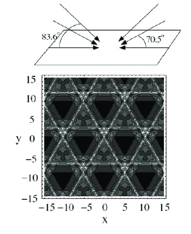
Figure 10: Laser setup (top) proposed in Ref. [42] to realize a trimerized kagome optical lattice (bottom). Figure adapted from [42].

7.1 Frustration can reveal “genuine” Mott physics

As mentioned above, frustration can help revealing Mott physics by pushing spin ordering to lower temperatures. One of the possible consequences is the appearance of a genuine (first-order) phase transition at finite temperature between a metallic (itinerant) phase at smaller $U/\rm{t}$ and a paramagnetic Mott insulating phase at large $U/\rm{t}$, as depicted in Fig. 7. Such a transition is indeed found within dynamical mean-field theory (DMFT), i.e in the limit of large lattice connectivity, for frustrated lattices. A first-order transition is observed in real materials as well (e.g in V₂O₃, cf. Fig. 6) but in this case the lattice degrees of freedom also participate (although the transition is indeed electronically driven). There are theoretical indications that, in the presence of frustration, a first order Mott transition at finite temperature exists for a rigid lattice beyond mean-field theory (see e.g [39]), but no solid proof either. In solid-state physics, it is not possible to suppress the coupling of electronic instabilities to lattice degrees of freedom, hence the experimental demonstration of this is hardly possible. This is a question that ultra-cold atomic systems might help answering.

The first-order transition line ends at a second-order critical endpoint: there is indeed no symmetry distinction between a metal and an insulator at finite temperature and it is logical that one can then find a continuous path from one to the other around the critical point. The situation is similar to the liquid-gas transition, and in fact it is expected that this phase transition is in the same universality class: that of the Ising model (this has been experimentally demonstrated for V₂O₃ [34]). A qualitative analogy with the liquid-gas transition can actually been drawn here: the Mott insulating phase has very few doubly occupied, or empty, sites (cf. the cartoons in Fig. 6) and hence corresponds to a low-density or gas phase (for double occupancies), while the metallic phase has many of them and corresponds to the higher-density liquid phase.

One can also ask whether it is possible to stabilize a paramagnetic Mott phase as the ground-state, i.e suppress spin ordering down to $T=0$. Several recent studies of frustrated two-dimensional models found this to happen at intermediate coupling $U/\rm{t}$ and for large enough frustration $\rm{t}^{\prime}/\rm{t}$, with non-magnetic insulating and possibly d-wave superconducting ground states arising (Fig. 11).

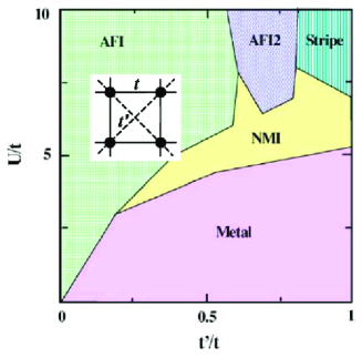
Figure 11: Ground-state phase diagram of the two-dimensional Hubbard model with nearest-neighbor and next nearest-neighbor hopping, as obtained in Ref. [38] from the “path-integral renormalization group method”. A non-magnetic Mott insulator (NMI) is stabilized for large enough frustration $\rm{t}^{\prime}/\rm{t}$ and intermediate coupling $U/\rm{t}$. A similar model with n.n.n hopping along only one of the diagonals (anisotropic triangular lattice) was studied in Ref. [32] using a cluster extension of DMFT, and an additional d-wave superconducting phase was found in this study.

7.2 Frustration can lead to exotic quantum magnetism

The above question of suppressing magnetic ordering down to $T=0$ due to frustration can also be asked in a more radical manner by considering the strong-coupling limit $U/\rm{t}\rightarrow\infty$. There, charge (density) fluctuations are entirely suppressed and the Hubbard model reduces to a quantum Heisenberg model. The question is then whether quantum fluctuations of the spin degrees of freedom only, can lead to a ground-state without long-range order. Studying this issue for frustrated Heisenberg models or related models has been a very active field of theoretical condensed matter physics for the past 20 years or so, and I simply direct the reader to existing reviews on the subject, e.g Ref. [37, 33]. Possible disordered phases are valence bond crystals, in which translational symmetry is broken and the ground-state can be qualitatively thought of as a specific paving of the lattice by singlets living on bonds. Another, more exotic, possibility is that the ground-state can be thought of as a resonant superposition of singlets (a sort of giant benzene molecule): this is the “resonating valence bond” idea proposed in the pioneering work of Anderson and Fazekas. There are a few examples of this, one candidate being the Heisenberg model on the kagome lattice (Fig. 10). Naturally, obtaining such unconventional states in ultra-cold atomic systems, and more importantly being able to measure the spin-spin correlations and excitation spectrum experimentally would be fascinating.

One last remark in this respect, which establishes an interesting connection between exotic quantum magnetism and Bose condensation. A spin-1/2 quantum Heisenberg model with a ground-state which is not ordered and does not break translational symmetry (e.g a resonating valence bond ground-state) is analogous, in a precise formal sense, to a specific interacting model of hard-core bosons which would remain a normal liquid (not a crystal, not a superfluid) down to $T=0$. Hence, somewhat ironically, an unconventional ground-state means, in the context of quantum magnetism, preventing Bose condensation. To see this, we observe that a quantum spin-1/2 can be represented with a hard-core boson operator $b_{i}$ as:

$$S^{+}_{i}=b^{\dagger}_{i}\,\,\,,\,\,\,S^{-}_{i}=b_{i}\,\,\,,\,\,\,S^{z}_{i}=b^{\dagger}_{i}b_{i}-\frac{1}{2}$$

with the constraint that at most one boson can live on a given site $b^{\dagger}_{i}b_{i}=0,1$ (infinite hard-core repulsion). The anisotropic Heisenberg (XXZ) model then reads:

$$H=J_{\perp}\sum_{\langle ij\rangle}[b^{\dagger}_{i}b_{j}+b^{\dagger}_{j}b_{i}]+J_{z}\sum_{\langle ij\rangle}(b^{\dagger}_{i}b_{i}-1/2)(b^{\dagger}_{j}b_{j}-1/2)$$

Hence, it is an infinite-U bosonic Hubbard model with an additional interaction between nearest-neighbor sites (note that dipolar interactions can generate those for real bosons). The superfluid phase for the bosons correspond to a phase with XY-order in the spin language, a crystalline (density-wave) phase with broken translational symmetry to a phase with antiferromagnetic ordering of the $S^{z}$ components, and a normal Bose fluid to a phase without any of these kinds of orders.

8 Quasiparticle excitations in strongly correlated fermion systems, and how to measure them.

8.1 Response functions and their relation to the spectrum of excitations

Perhaps even more important than the nature of the ground-state of a many-body system is to understand the nature of the excited states, and particularly of the low-energy excited states (i.e close to the ground-state). Those are the states which control the response of the system to a weak perturbation, which is what we do when we perform a measurement without disturbing the system too far out of equilibrium . When the perturbation is weak, linear response theory can be used, and in the end what is measured is the correlation function of some observable (i.e of some operator $\hat{O}$):

$$C_{O}(\mathbf{r},\mathbf{r}^{\prime};t,t^{\prime})\,=\,\langle\hat{O}(\mathbf{r},t)\,\hat{O}^{\dagger}(\mathbf{r}^{\prime},t^{\prime})\rangle$$ (47)

In this expression, the operators evolve in the Heisenberg representation, and the brackets denote either an average in the ground-state (many-body) wave function (for a measurement at $T=0$) or, at finite temperature, a thermally weighted average with the equilibrium Boltzmann weight. How the behaviour of this correlation function is controlled by the spectrum of excited states is easily understood by inserting a complete set of states in the above expression (in order to make the time evolution explicit) and obtaining the following spectral representation (given here at $T=0$ for simplicity):

$$C_{O}(\mathbf{r},\mathbf{r}^{\prime};t,t^{\prime})\,=\,\sum_{n}e^{-\frac{i}{\hbar}(E_{n}-E_{0})(t-t^{\prime})}\,\langle\Phi_{0}|\hat{O}(\mathbf{r})|\Phi_{n}\rangle\langle\Phi_{n}|\hat{O}(\mathbf{r}^{\prime})^{\dagger}|\Phi_{0}\rangle$$ (48)

In this expression, $\Phi_{0}$ is the ground-state (many-body) wave function, and the summation is over all admissible many-body excited states (i.e having non-zero matrix elements).

A key issue in the study of ultra-cold atomic systems is to devise measurement techniques in order to probe the nature of these many-body states. In many cases, one can resort to spectroscopic techniques, quite similar in spirit to what is done in condensed matter physics. This is the case, for example, when the observable $\hat{O}$ we want to access is a local observable such as the local density or the local spin-density. Light (possibly polarized) directly couples to those, and light scattering is obviously the tool of choice in the context of cold atomic systems. Bragg scattering [44] can be indeed used to measure the density-density dynamical correlation function $\langle\rho(\mathbf{r},t)\rho(\mathbf{r}^{\prime},t^{\prime})\rangle$ and polarized light also allows one to probe [7] the spin-spin response $\langle\mathbf{S}(\mathbf{r},t)\mathbf{S}^{\prime}(\mathbf{r}^{\prime},t^{\prime})\rangle$. In condensed matter physics, analogous measurements can be done by light or neutron scattering.

One point is worth emphasizing here, for condensed matter physicists. In condensed matter physics, we are used to thinking of visible or infra-red light (not X-ray !) as a zero-momentum probe, because the wavelength is much bigger than inter-atomic distances. This is not the case for atoms in optical lattices ! For those, the lattice spacing is set by the wavelength of the laser, hence lasers in the same range of wavelength can be used to sample the momentum-dependence of various observables, with momentum transfers possibly spanning the full extent of the Brillouin zone.

Other innovative measurement techniques of various two-particle correlation functions have recently been proposed and experimentally demonstrated in the context of ultra-cold atomic systems, some of which are reviewed elsewhere in this set of lectures, e.g noise correlation measurements [1, 14, 20], or periodic modulations of the lattice [46, 28].

The simplest examples we have just discussed involve two-particle correlation functions (density-density, spin-spin), and hence probe at low energy the spectrum of particle-hole excitations, i.e excited states $\Phi_{n}$ which are coupled to the ground-state via an operator conserving particle number. In contrast, one may want to probe one-particle correlation functions, which probe excited states of the many-body system with one atom added to it, or one atom removed, i.e coupled to the ground-state via a single particle process. Such a correlation function (also called the single-particle Green’s function $G_{1}$) reads:

$$\langle T_{t}\psi(\mathbf{r},t)\psi^{\dagger}\,(\mathbf{r}^{\prime},t^{\prime})\rangle\equiv i\,G_{1}(\mathbf{r},\mathbf{r}^{\prime};t,t^{\prime})$$ (49)

in which $T_{t}$ denotes time ordering. The corresponding spectral decomposition involves the one-particle spectral function (written here, for simplicity, for a homogeneous system -so that crystal momentum is a good quantum number- and at $T=0$):

$$A(\mathbf{k},\omega)= \sum_{n}|\langle\Phi_{n}^{N-1}|c_{\,\mathbf{k}}|\Phi_{0}^{N}\rangle|^{2}\,\delta(\omega+\mu+E_{n}-E_{0})\,\,\,(\omega<0)$$

$$= \sum_{n}|\langle\Phi_{n}^{N+1}|c_{\,\mathbf{k}}^{\dagger}|\Phi_{0}^{N}\rangle|^{2}\,\delta(\omega+\mu+E_{0}-E_{n})\,\,\,(\omega>0)$$ (50)

The spectral function is normalized to unity for each momentum, due to the anticommutation of fermionic operators:

$$\int_{-\infty}^{+\infty}A(\mathbf{k},\omega)\,d\omega=1$$ (51)

As explained in the next section, the momentum and frequency dependence of this quantity contains key information about the important low-energy excitations of fermionic systems (hole-like, i,e corresponding to the removal of one atom, for $\omega<0$, and particle-like for $\omega>0$). Let us note that, for Bose systems with a finite condensate density $n_{0}$, the two-particle correlators are closely related to the one-particle correlators via terms such as $n_{0}\,\langle\psi^{\dagger}(\mathbf{r},t)\,\psi(\mathbf{r}^{\prime},t^{\prime})\rangle$. By contrast, in Fermi systems the distinction between one- and two-particle correlators is essential.

A particular case is the equal-time correlator, $\langle\psi^{\dagger}(\mathbf{r},t)\psi(\mathbf{r}^{\prime},t)\rangle$, i.e the one-body density matrix, whose Fourier transform is the momentum distribution in the ground-state:

$$N(\mathbf{k})=\langle\Phi_{0}|c^{\dagger}_{\mathbf{k}}\,c_{\mathbf{k}}|\Phi_{0}\rangle=\int_{-\infty}^{0}A(\mathbf{k},\omega)d\omega$$ (52)

For ultra-cold atoms, this can be measured in time of flight experiments. Conversely, rf-spectroscopy experiments [8] give some access to the frequency dependence of the one-particle spectral function, but not to its momentum dependence.

8.2 Measuring one-particle excitations by stimulated Raman scattering

In condensed matter physics, angle-resolved photoemission spectroscopy (ARPES) provides a direct probe of the one-particle spectral function (for a pedagogical introduction, see [9]). This technique has played a key role in revaling the highly unconventional nature of single-particle excitations in cuprate superconductors [10]. It consists in measuring the energy and momentum of electrons emitted out of the solid exposed to an incident photon beam. In the simplest approximation, the emitted intensity is directly proportional to the single-electron spectral function (multiplied by the Fermi function and by some matrix elements).

In Ref. [11], it was recently proposed to use stimulated Raman spectroscopy as a probe of one-particle excitations, and of the frequency and momentum dependence of the spectral function, in a two-component mixture of ultracold fermionic atoms in two internal states $\alpha$ and $\alpha^{\prime}$. Stimulated Raman spectroscopy has been considered previously in the context of cold atomic gases, both as an outcoupling technique to produce an atom laser [21] and as a measurement technique for bosons [25, 35, 3, 36] and fermions [47, 50]. In the Raman process of Fig. 12, atoms are transferred from $\alpha$ into another internal state $\beta\neq\alpha,\alpha^{\prime}$, through an intermediate excited state $\gamma$, using two laser beams of wavectors $\mathbf{k}_{1,2}$ and frequencies $\omega_{1,2}$. If $\omega_{1}$ is sufficiently far from single photon resonance to the excited $\gamma$ state, we can neglect spontaneous emission. The total transfer rate to state $\beta$ can be calculated [25, 35, 3] using the Fermi golden rule and eliminating the excited state:

$$R(\mathbf{q},\Omega)=|C|^{2}n_{1}(n_{2}+1)\int_{-\infty}^{\infty}\,dt\int\!d\mathbf{r}\,d\mathbf{r}^{\prime}\,e^{i[\,\Omega\,t-\mathbf{q}\cdot(\mathbf{r}-\mathbf{r}^{\prime})]}\,g_{\beta}(\mathbf{r},\mathbf{r}^{\prime};t)\langle\psi^{+}_{\alpha}(\mathbf{r},t)\psi_{\alpha}(\mathbf{r}^{\prime},0)\rangle$$

Here $\mathbf{q}=\mathbf{k}_{1}-\mathbf{k}_{2}$ and $\Omega=\omega_{1}-\omega_{2}+\mu$ with $\mu$ the chemical potential of the interacting gas, and $n_{1,2}$ the photon numbers present in the laser beams. Assuming that no atoms are initially present in $\beta$ and that the scattered atoms in $\beta$ do not interact with the atoms in the initial $\alpha,\alpha^{\prime}$ states, the free propagator for $\beta$-state atoms in vacuum is to be taken: $g_{\beta}(\mathbf{r},\mathbf{r}^{\prime};t)\equiv\langle 0_{\beta}|\,\psi_{\beta}(\mathbf{r},t)\psi^{\dagger}_{\beta}(\mathbf{r}^{\prime},0)|0_{\beta}\rangle$. For a uniform system, the transfer rate can be related to the spectral function $A(\mathbf{k},\omega)$ of atoms in the internal state $\alpha$ by [35]:

$$R(\mathbf{q},\Omega)\propto\,\int\!d\mathbf{k}\,n_{F}\,(\varepsilon_{\mathbf{k}\beta}-\Omega)\,A(\mathbf{k}-\mathbf{q},\varepsilon_{\mathbf{k}\beta}-\Omega)$$ (53)

in which the Green’s function has been expressed in terms of the spectral function and the Fermi factor $n_{F}$. In the presence of a trap, the confining potential can be treated in the local density approximation by integrating the above expression over the radial coordinate, with a position-dependent chemical potential. From (53), the similarities and differences with ARPES are clear: in both cases, an atom is effectively removed from the interacting gas, and the signal probes the spectral function. In the case of ARPES, it is directly proportional to it, while here an additional momentum integration is involved if the atoms in state $\beta$ remain in the trap. One the other hand, in the present context, one can in principle vary the momentum transfer $\mathbf{q}$ and regain momentum resolution in this manner. Alternatively, one can cut off the trap and perform a time of flight experiment [11], in which case the measured rate is directly proportional to $n_{F}\,(\varepsilon_{\mathbf{k}\beta}-\Omega)\,A(\mathbf{k}-\mathbf{q},\varepsilon_{\mathbf{k}\beta}-\Omega)$, in closer analogy to ARPES. Varying the frequency shift $\Omega$ then allows to sample different regions of the Brillouin zone [11].

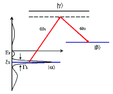
Figure 12: Raman process: transfer from an internal state $\alpha$ to another internal state $\beta$ through an excited state $\gamma$. The momentum-resolved spectral function is schematized, consisting of a quasiparticle peak and an incoherent background. From Ref. [11].

8.3 Excitations in interacting Fermi systems: a crash course

Most interacting fermion systems have low-energy excitations which are well-described by “Fermi liquid theory” which is a low-energy effective theory of these excitations. In this description, the low-energy excitations are built out of quasiparticles, long-lived (coherent) entities carrying the same quantum numbers than the original particles. There are three key quantities characterizing the quasiparticle excitations:

• Their dispersion relation, i.e the energy $\xi_{\mathbf{k}}$ (measured from the ground-state energy) necessary to create such an excitation with (quasi-) momentum $\mathbf{k}$. The interacting system possesses a Fermi surface (FS) defined by the location in momentum space on which the excitation energy vanishes: $\xi_{\mathbf{k}_{F}}=0$. Close to a given point on the FS, the quasiparticle energy vanishes as: $\xi_{\mathbf{k}}\sim\mathbf{v}_{F}(\mathbf{k}_{F})\cdot(\mathbf{k}-\mathbf{k}_{F})+\cdots$, with $\mathbf{v}_{F}$ the local Fermi velocity at that given point of the Fermi surface.

• The spectral weight $Z_{\mathbf{k}}\leq 1$ carried by these quasiparticle excitations, in comparison to the total spectral weight ($=1$, see above) of all one-particle excited states of arbitrary energy and fixed momentum.

• Their lifetime $\Gamma_{\mathbf{k}}^{-1}$. It is finite away from the Fermi surface, as well as at finite temperature. The quasiparticle lifetime diverges however at $T=0$ as $\mathbf{k}$ gets close to the Fermi surface. Within Fermi liquid theory, this happens in a specific manner (for phase-space reasons), as $\Gamma_{\mathbf{k}}\sim\xi_{\mathbf{k}}^{2}$. This insures the overall coherence of the description in terms of quasiparticles, since their inverse lifetime vanishes faster than their energy.

Typical signatures of strong correlations are the following effects (not necessarily occurring simultaneously in a given system): i) strongly renormalized Fermi velocities, as compared to the non-interacting (band) value, corresponding e.g to a large interaction-induced enhancement of the effective mass of the quasiparticles, ii) a strongly suppressed quasiparticle spectral weight $Z_{\mathbf{k}}\ll 1$, possibly non-uniform along the Fermi surface, iii) short quasiparticle lifetimes. These strong deviations from the non-interacting system can sometimes be considerable: the “heavy fermion” materials for example (rare-earth compounds) have quasiparticle effective masses which are several hundred times bigger than the mass from band theory, and in spite of this are mostly well described by Fermi liquid theory.

The quasiparticle description applies only at low energy, below some characteristic energy (and temperature) scale $T_{F}^{\star}$, the quasiparticle coherence scale. Close to the Fermi surface, the one-particle spectral function displays a clear separation of energy scales, with a sharp coherent peak carrying spectral weight $Z_{\mathbf{k}}$ corresponding to quasiparticles (a peak well-resolved in energy means long-lived excitations), and an “incoherent” background carrying spectral weight $1-Z_{\mathbf{k}}$. A convenient form to have in mind (Fig. 12) is:

$$A(\mathbf{k},\omega)\,\simeq\,Z_{\mathbf{k}}\,\frac{\Gamma_{\mathbf{k}}}{\pi[(\omega-\xi_{\mathbf{k}})^{2}+\Gamma_{\mathbf{k}}^{2}]}\,+\,A_{\rm{inc}}(\mathbf{k},\omega)$$ (54)

Hence, measuring the spectral function, and most notably the evolution of the quasiparticle peak as the momentum is swept through the Fermi surface, allows one to probe the key properties of the quasiparticle excitations: their dispersion (position of the peak), lifetime (width of the peak) and spectral weight (normalized to the incoherent background, when possible), as well of course as the location of the Fermi surface of the interacting system in the Brillouin zone. In [11], it was shown that the shape of the Fermi surface, as well as some of the quasiparticle properties can be determined, in the cold atoms context, from the Raman spectroscopy described above. For the pioneering experimental determination of Fermi surfaces in weakly or non-interacting fermionic gases in optical lattices, see [27].

What about the “incoherent” part of the spectrum (which in a strongly correlated system may carry most of the spectral weight…) ? Close to the Mott transition, we expect at least one kind of well-defined high energy excitations to show up in this incoherent spectrum. These are the excitations which consist in removing a particle from a site which is already occupied, or adding a particle on such a site. The energy difference separating these two excitations is precisely the Hubbard interaction $U$. These excitations, which are easier to think about in a local picture in real-space (in contrast to the wave-like, quasiparticle excitations), form two broad dispersing peaks in the spectral functions: the so-called Hubbard “bands”.

In the mean-field (DMFT) description of interacting fermions and of the Mott transition, the quasiparticle weight $Z$ is uniform along the Fermi surface. Close to the Mott transition, $Z$ vanishes and the effective mass ($m^{\star}/m=1/Z$ in this theory) of quasiparticles diverges. The quasiparticle coherence scale is $T_{F}^{\star}\simeq Z\,T_{F}$, with $T_{F}$ the Fermi energy ($\sim$ bandwidth) of the non-interacting system: this coherence scale also becomes very small close to the transition, and Hubbard bands carry most of the spectral weight in this regime.

8.4 Elusive quasiparticles and nodal-antinodal dichotomy: the puzzles of cuprate superconductors

The cuprate superconductors, which are quasi two-dimensional doped Mott insulators, raise some fundamental questions about the description of excitations in strongly interacting fermion systems. In the “normal” (i.e non-superconducting) state of these materials, strong departure from Fermi liquid theory is observed. Most notably, at doping levels smaller than the optimal doping (where the superconducting $T_{c}$ is maximum), i.e in the so-called “underdoped” regime:

• Reasonably well-defined quasiparticles are only observed close to the diagonals of the Brillouin zone, i.e close to the “nodal points” of the Fermi surface where the superconducting gap vanishes. Even there, the lifetimes are shorter and appear to have a different energy and temperature dependence than that of Fermi liquid theory.

• In the opposite regions of the Fermi surface (“antinodal” regions), the spectral function shows no sign of a quasiparticle pleak in the normal state. Instead, a very broad lineshape is found in ARPES, whose leading edge is not centered at $\omega=0$, but rather at a finite energy scale. The spectral function appears to have its maximum away from the Fermi surface, i.e the density of low-energy excitations is strongly depleted at low-energy: this is the “pseudo-gap” phenomenon. The pseudo-gap shows up in many other kinds of measurements in the under-doped regime.

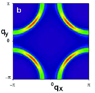
Figure 13: Illustration of the dichotomy between “nodal” and “antinodal” regions of the Fermi surface, as observed in cuprate superconductors. Colour coding corresponds to increasing intensity of the quasiparticle peak. Such effects could be revealed in cold atomic systems by stimulated Raman spectroscopy measurements, as proposed in Ref. [11].

Hence, there is a strong dichotomy between the nodal and antinodal regions in the normal state. The origin of this dichotomy is one of the key issues in the field. One possibility is that the pseudo-gap is due to a hidden form of long-range order which competes with superconductivity and is responsible for suppressing excitations except in nodal regions. Another possibility is that, because of the proximity to the Mott transition in such low-dimensional systems, the quasiparticle coherence scale (and most likely also the quasiparticle weight) varies strongly along the Fermi surface, hence suppressing quasiparticles in regions where the coherence scale is smaller than temperature.

This nodal-antinodal dichotomy is illustrated in Fig. 13. This figure has actually been obtained from a simulated intensity plot of the Raman rate (53), using a phenomenological form of the spectral function appropriate for cuprates. It is meant to illustrate how future experiments on ultra-cold fermionic atoms in two-dimensional optical lattices might be able to address some of the fundamental issues in the physics of strongly correlated quantum systems.

- [1] E. Altman, E. Demler, and M. D. Lukin, Probing many-body states of ultracold atoms via noise correlations, Phys. Rev. A 70 (2004), no. 1, 013603.
- [2] G. G. Batrouni, V. Rousseau, R. T. Scalettar, M. Rigol, A. Muramatsu, P. J. H. Denteneer, and M. Troyer, Mott domains of bosons confined on optical lattices, Phys. Rev. Lett. 89 (2002), no. 11, 117203.
- [3] P. Blair Blakie, Raman Spectroscopy of Mott insulator states in optical lattices, ArXiv Condensed Matter e-prints (2005).
- [4] P. B. Blakie and A. Bezett, Adiabatic cooling of Fermions in an optical lattice, Phys. Rev. A 71 (2005), 033616.
- [5] I. Bloch, Ultracold quantum gases in optical lattices, Nature Physics 1 (2005), 24.
- [6] T. Bourdel, L. Khaykovich, J. Cubizolles, J. Zhang, F. Chevy, M. Teichmann, L. Tarruell, S. J. Kokkelmans, and C. Salomon, Experimental Study of the BEC-BCS Crossover Region in Lithium 6, Phys. Rev. Lett. 93 (2004), no. 5, 050401.
- [7] I. Carusotto, Bragg scattering and the spin structure factor of two-component atomic gases, J. Phys. B: At.Mol.Opt.Phys. 39 (2006), S211.
- [8] C. Chin, M. Bartenstein, A. Altmeyer, S. Riedl, S. Jochim, J. H. Denschlag, and R. Grimm, Observation of the Pairing Gap in a Strongly Interacting Fermi Gas, Science 305 (2004), 1128.
- [9] A. Damascelli, Probing the Electronic Structure of Complex Systems by ARPES, Physica Scripta Volume T 109 (2004), 61.
- [10] A. Damascelli, Z. Hussain, and Z.-X. Shen, Angle-resolved photoemission studies of the cuprate superconductors, Rev. Mod. Phys. 75 (2003), 473.
- [11] T.-L. Dao, A. Georges, J. Dalibard, C. Salomon, and I. Carusotto, Measuring the one-particle excitations of ultracold fermionic atoms by stimulated Raman spectroscopy, ArXiv Condensed Matter e-prints (2006).
- [12] A-M. Daré, L. Raymond, G. Albinet, and A.-M. S. Tremblay, Interaction-induced adiabatic cooling for antiferromagnetism in optical lattices, preprint (2006).
- [13] M. P. A. Fisher, P. B. Weichman, G. Grinstein, and D. S. Fisher, Boson localization and the superfluid-insulator transition, Phys. Rev. B 40 (1989), 546.
- [14] S. Fölling, F. Gerbier, A. Widera, O. Mandel, T. Gericke, and I. Bloch, Spatial quantum noise interferometry in expanding ultracold atom clouds, Nature 434 (2005), 481.
- [15] S. Fölling, A. Widera, T. Müller, F. Gerbier, and I. Bloch, Formation of Spatial Shell Structure in the Superfluid to Mott Insulator Transition, Phys. Rev. Lett. 97 (2006), no. 6, 060403.
- [16] A. Georges, Strongly Correlated Electron Materials: Dynamical Mean-Field Theory and Electronic Structure, Lectures on the physics of highly correlated electron systems VIII (A. Avella and F. Mancini, eds.), American Institute of Physics, 2004, cond-mat/0403123.
- [17] A. Georges, G. Kotliar, W. Krauth, and M. J. Rozenberg, Dynamical mean-field theory of strongly correlated fermion systems and the limit of infinite dimensions, Reviews of Modern Physics 68 (1996), 13–125.
- [18] M. Greiner, O. Mandel, T. Esslinger, T. W. Hänsch, and I. Bloch, Quantum phase transition from a superfluid to a mott insulator in a gas of ultracold atoms, Nature 415 (2002), 39.
- [19] M. Greiner, C. A. Regal, and D. S. Jin, Emergence of a molecular bose-einstein condensate from a fermi gas, Nature 537 (2003), 426.
- [20] M. Greiner, C. A. Regal, J. T. Stewart, and D. S. Jin, Probing pair-correlated fermionic atoms through correlations in atom shot noise, Phys. Rev. Lett. 94 (2005), no. 11, 110401.
- [21] E. W. Hagley, L. Deng, M. Kozuma, J. Wen, K. Helmerson, S. L. Rolston, and W. D. Phillips, A well-collimated quasi-continuous atom laser, Science 283 (1999), 1706.
- [22] W. Hofstetter, J. I. Cirac, P. Zoller, E. Demler, and M. D. Lukin, High-temperature superfluidity of fermionic atoms in optical lattices, Phys. Rev. Lett. 89 (2002), no. 22, 220407.
- [23] D. Jaksch, C. Bruder, J. I. Cirac, C. W. Gardiner, and P. Zoller, Cold Bosonic Atoms in Optical Lattices, Phys. Rev. Lett. 81 (1998), 3108–3111.
- [24] D. Jaksch and P. Zoller, The cold atom Hubbard toolbox, Annals of Physics 315 (2005), 52.
- [25] Y. Japha, S. Choi, K. Burnett, and Y. B. Band, Coherent Output, Stimulated Quantum Evaporation, and Pair Breaking in a Trapped Atomic Bose Gas, Phys. Rev. Lett. 82 (1999), 1079–1083.
- [26] S. Jochim, M. Bartenstein, A. Altmeyer, Hendl G., Riedl S., C. Chin, J. H. Denschlag, and R. Grimm, Bose-einstein condensation of molecules, Science 302 (2003), 2101.
- [27] M. Köhl, H. Moritz, T. Stöferle, K. Günter, and T. Esslinger, Fermionic atoms in a 3D optical lattice: Observing Fermi-surfaces, dynamics and interactions, Phys. Rev. Lett. 94 (2005), 080403.
- [28] C. Kollath, A. Iucci, T. Giamarchi, W. Hofstetter, and U. Schollwock, Spectroscopy of ultracold atoms by periodic lattice modulations, Phys. Rev. Lett. 97 (2006), no. 5, 050402.
- [29] G. Kotliar, Driving the electron over the edge, Science 302 (2003), 67.
- [30] G. Kotliar and D. Vollhardt, Strongly correlated electron materials: insights from dynamical mean field theory, Physics Today March 2004 (2004), 53.
- [31] W. Krauth, M. Caffarel, and J.-P. Bouchaud, Gutzwiller wave function for a model of strongly interacting bosons, Phys. Rev. B 45 (1992), 3137–3140.
- [32] B. Kyung and A.-M. S. Tremblay, Mott transition, antiferromagnetism, and d-wave superconductivity in two-dimensional organic conductors, Phys. Rev. Lett. 97 (2006), no. 4, 046402.
- [33] C. Lhuillier, Frustrated Quantum Magnets, ArXiv Condensed Matter e-prints (2005).
- [34] P. Limelette, A. Georges, D. Jérome, P. Wzietek, P. Metcalf, and J. M. Honig, Universality and Critical Behavior at the Mott Transition, Science 302 (2003), 89–92.
- [35] D. L. Luxat and A. Griffin, Coherent tunneling of atoms from Bose-condensed gases at finite temperatures, Phys. Rev. A 65 (2002), no. 4, 043618.
- [36] I. E. Mazets, G. Kurizki, N. Katz, and N. Davidson, Optically Induced Polarons in Bose-Einstein Condensates: Monitoring Composite Quasiparticle Decay, Physical Review Letters 94 (2005), no. 19, 190403.
- [37] G. Misguich and C. Lhuillier, Frustrated spin systems, ch. Two-dimensional quantum antiferromagnets, World Scientific, Singapore, 2003, cond-mat/0310405.
- [38] T. Mizusaki and M. Imada, Gapless quantum spin liquid, stripe, and antiferromagnetic phases in frustrated hubbard models in two dimensions, Phys. Rev. B 74 (2006), no. 1, 014421.
- [39] O. Parcollet, G. Biroli, and G. Kotliar, Cluster dynamical mean field analysis of the mott transition, Phys. Rev. Lett. 92 (2004), 226402.
- [40] K. I. Petsas, A. B. Coates, and G. Grynberg, Crystallography of optical lattices, Phys. Rev. A 50 (1994), no. 6, 5173–5189.
- [41] D. S. Rokhsar and B. G. Kotliar, Gutzwiller projection for bosons, Phys. Rev. B 44 (1991), 10328.
- [42] L. Santos, M. A. Baranov, J. I. Cirac, H.-U. Everts, H. Fehrmann, and M. Lewenstein, Atomic quantum gases in kagome lattices, Phys. Rev. Lett. 93 (2004), no. 3, 030601.
- [43] K. Sheshadri, H. R. Krishnamurthy, R. Pandit, and T. V. Ramakrishnan, Superfluid and insulating phases in an interacting-boson model: mean-field theory and the RPA, Europhysics Letters 22 (1993), 257.
- [44] D. M. Stamper-Kurn, A. P. Chikkatur, A. Görlitz, S. Inouye, S. Gupta, D. E. Pritchard, and W. Ketterle, Excitation of phonons in a bose-einstein condensate by light scattering, Phys. Rev. Lett. 83 (1999), no. 15, 2876.
- [45] R. Staudt, M. Dzierzawa, and A. Muramatsu, Phase-diagram of the three-dimensional hubbard model at half-filling, Eur. Phys. J. B 17 (2000), 411.
- [46] Thilo Stoferle, Henning Moritz, Christian Schori, Michael Kohl, and Tilman Esslinger, Transition from a strongly interacting 1d superfluid to a mott insulator, Phys. Rev. Lett. 92 (2004), no. 13, 130403.
- [47] P. Törmä and P. Zoller, Laser Probing of Atomic Cooper Pairs, Physical Review Letters 85 (2000), 487–490.
- [48] F. Werner, Antiferromagnétisme d’atomes froids fermioniques dans un réseau optique, unpublished Master report (2004).
- [49] F. Werner, O. Parcollet, A. Georges, and S. R. Hassan, Interaction-induced adiabatic cooling and antiferromagnetism of cold fermions in optical lattices, Phys. Rev. Lett. 95, 056401.
- [50] W. Yi and L. . Duan, Detecting the breached pair phase in a polarized ultracold Fermi gas, ArXiv Condensed Matter e-prints (2006).
- [51] W. Zwerger, Mott-Hubbard transition of cold atoms in optical lattices, Journal of Optics B: Quantum and Semiclassical Optics 5 (2003), 9.
- [52] M. W. Zwierlein, C. A. Stan, C. H. Schunck, S. M. Raupach, S. Gupta, Z. Hadzibabic, and W. Ketterle, Observation of Bose-Einstein Condensation of Molecules, Phys. Rev. Lett. 91 (2003), no. 25, 250401.