Phaseless auxiliary-field quantum Monte Carlo calculations with planewaves and pseudopotentials—applications to atoms and molecules

Abstract

The phaseless auxiliary-field quantum Monte Carlo (AF QMC) method [S. Zhang and H. Krakauer, Phys. Rev. Lett. 90, 136401 (2003)] is used to carry out a systematic study of the dissociation and ionization energies of second-row group 3A-7A atoms and dimers, Al, Si, P, S, Cl. In addition, the P₂ dimer is compared to the third-row As₂ dimer, which is also triply-bonded. This method projects the many-body ground state by means of importance-sampled random walks in the space of Slater determinants. The Monte Carlo phase problem, due to the electron-electron Coulomb interaction, is controlled via the phaseless approximation, with a trial wave function $|\Psi_{T}\rangle$. As in previous calculations, a mean-field single Slater determinant is used as $|\Psi_{T}\rangle$. The method is formulated in the Hilbert space defined by any chosen one-particle basis. The present calculations use a planewave basis under periodic boundary conditions with norm-conserving pseudopotentials. Computational details of the planewave AF QMC method are presented. The isolated systems chosen here allow a systematic study of the various algorithmic issues. We show the accuracy of the planewave method and discuss its convergence with respect to parameters such as the supercell size and planewave cutoff. The use of standard norm-conserving pseudopotentials in the many-body AF QMC framework is examined.

I Introduction

Achieving accurate solutions of the electronic many-body Schrödinger equation is a challenging problem for calculations of the properties of real materials. For many systems, density functional theory (DFT), in a variety of approximations, has been applied with great success. In DFT, the many-body interactions are replaced by a single particle interacting with the mean-field generated by the other particles, similar in spirit to the Hartree-Fock (HF) method. Unfortunately, these methods have well-known limitations and often fail at describing the properties of materials with large electron-electron correlation.

A more accurate approach is the quantum Monte Carlo (QMC) method Ceperley and Alder (1980); Reynolds et al. (1982); Foulkes et al. (2001); Zhang and Krakauer (2003), which has been shown to be among the most effective methods for many-electron problems. Unlike other correlated methods, QMC calculation times scale as a low power of the system size Williamson et al. (2001). The fixed-node diffusion Monte Carlo (DMC) approach, which samples the many-body wave function in real space, has been the most widely used QMC method in electronic structure calculations Reynolds et al. (1982); Foulkes et al. (2001).

The recently developed phaseless auxiliary-field quantum Monte Carlo (AF QMC) method Zhang and Krakauer (2003) is an alternative and complementary QMC approach, which samples the many-body wave function in the space of Slater determinants. This method has several attractive features. The fermionic antisymmetry of the wave function is automatically accounted for, since it is sampled by Slater determinants. This provides a different route to controlling the sign problem Ceperley and Alder (1984); Zhang and Kalos (1991); Zhang (1999) from fixed-node DMC, which has shown promise in reducing the dependence of the systematic errors on the trial wave function Al-Saidi et al. (2006a, b, c). The orbitals in the Slater determinants are expressed in terms of a chosen single-particle basis (e.g., planewaves, Gaussians, etc.), so AF QMC shares much of the same computational machinery with DFT and other independent-particle type methods. AF QMC can thus straightforwardly incorporate many of the methodological advances from mean-field methods (such as pseudopotential and fast Fourier transforms) while systematically improving on mean-field accuracy.

Using a planewave basis, tests of the phaseless AF QMC method for a few simple atoms and molecules Zhang and Krakauer (2003); Zhang et al. (2005) as well as for the more correlated TiO and MnO molecules Al-Saidi et al. (2006a) yielded excellent results. More systematic applications of the phaseless AF QMC method to atoms and molecules have been carried out using Gaussian basis sets. These include all-electron calculations for first-row systems Al-Saidi et al. (2006b) and effective-core potential calculations in post-$d$ group elements Al-Saidi et al. (2006c). The results also showed excellent agreement with near-exact quantum chemistry results and/or experiment.

The planewave AF QMC method is well-adaped for correlated calculations of extended bulk systems, where planewave based methods have been the standard choice in traditional electronic structure calculations. It is therefore important to systematically study its algorithmic issues and to characterize its performance. In this paper, we use the planewave phaseless AF QMC method to carry out a systematic study of the dissociation and ionization energies of second-row atoms and dimers in Group 3A-7A, namely Al, Si, P, S, Cl. The interesting case of the triply-bonded P₂ dimer is also compared to the third-row As₂ dimer. The principal goal of this study is to further benchmark the AF QMC method across more systems and across different basis sets and to compare the results with those from other methods and experiment. While the use of localized basis sets, such as Gaussians, is generally more efficient for isolated atoms and molecules, it is straighforward to apply planewave methods using periodic boundary conditions and large supercells. Planewave methods have several desirable features. A planewave basis provides an unbiased representation of the wave functions, since convergence to the infinite basis limit is controlled by a single parameter, the kinetic-energy cutoff $E_{\textrm{cut}}$. Planewaves are algorithmically simple to implement, and operations with planewaves can be made very efficient, using fast Fourier techniques as in DFT methods. To keep the planewave basis size tractable, pseudopotentials must be used to eliminate the highly localized core electron states and to produce relatively smooth valence wave functions. The present choice of isolated atomic and molecular systems permits direct comparisons with Gaussian-based AF QMC and with well-establised quantum chemistry all-electron and pseudopotential calculations.

The remainder of this paper is organized as follows. In Section II, we describe computational details of the phaseless AF QMC method in the planewave-pseudopotential framework. In Section III, we discuss calculation parameters such as supercell (simulation cell) size, cutoff energy, and AF QMC time step size, and the algorithm’s convergence behavior with respect to these parameters. Section IV presents the calculated dissociation and ionization energies and comparisons with other theoretical results and with experiment. In Section V, we discuss systematic errors due to the use of the phaseless approximation and use of norm-conserving pseudopotentials. We then conclude with some general remarks in Section VI.

II Planewave AF QMC method: Computational Details

II.1 Hamiltonian

It is convenient to express, within the Born Oppenheimer approximation, the electronic Hamiltonian in second quantized form in terms of a chosen orthonormal one-particle basis

$${\hat{H}}=\sum_{ij}^{M}{H^{(1)}_{ij}c_{{i}}^{\dagger}c_{{j}}}+\frac{1}{2}\sum_{ijkl}^{M}{H^{(2)}_{ijkl}c_{{i}}^{\dagger}c_{{j}}^{\dagger}c_{{l}}c_{{k}}}+V_{\textrm{II}}\,,$$ (1)

where $M$ is the number of basis functions, $c_{i}^{\dagger}$ and $c_{i}$ are the corresponding creation and annihilation operators, and the electron spins have been subsumed in the summations. $H^{(1)}_{ij}$ and $H^{(2)}_{ijkl}$ are the one- and two-body matrix elements, and $V_{\textrm{II}}$ is the classical Coulomb interaction of the point ions Yin and Cohen (1982). Atomic units are used throughout this paper. We use periodic boundary conditions and a planewave basis

$$\langle{{\mathbf{r}}}|{{\mathbf{G}}}\rangle\equiv\langle{{{\mathbf{r}}}}|{{\,c_{{\mathbf{G}}}^{\dagger}}}|{{0}}\rangle=\frac{1}{{\sqrt{\Omega}}}\exp(i{\mathbf{G}}\cdot{\mathbf{r}})\,,$$ (2)

where $\Omega$ is the volume of the simulation cell and ${\mathbf{G}}$ is a reciprocal lattice vector. As in planewave-based density functional calculations, the number of planewaves $M$ in the basis is determined $G^{2}/2\leq E_{\textrm{cut}}$, where $E_{\textrm{cut}}$ is the cutoff kinetic energy.

The one-body operators in the Hamiltonian include the kinetic energy,

$${\hat{K}}=\frac{1}{2}\sum_{\mathbf{G}}{G^{2}}\,c_{{\mathbf{G}}}^{\dagger}c_{{\mathbf{G}}}\,,$$ (3)

and nonlocal pseudopotential, which describes the electron-ion interaction

$$\begin{split}\hat{V}_{\textrm{ei}}&=\sum_{\mathbf{G},\mathbf{G}^{\prime}}V_{\textrm{L}}({\mathbf{G}}-{\mathbf{G}^{\prime}})\,c_{{\mathbf{G}}}^{\dagger}c_{{\mathbf{G}^{\prime}}}\\ &\,+\sum_{\mathbf{G},\mathbf{G}^{\prime}}V_{\textrm{NL}}({\mathbf{G}},{\mathbf{G}}^{\prime})\,c_{{\mathbf{G}}}^{\dagger}c_{{\mathbf{G}^{\prime}}}\,,\end{split}$$ (4)

where $V_{\textrm{L}}({\mathbf{G}}-{\mathbf{G}^{\prime}})$ and $V_{\textrm{NL}}({\mathbf{G}},{\mathbf{G}^{\prime}})$ are the matrix elements of local and nonlocal parts of the pseudopotential, respectively. It is convenient to rewrite the local part of the pseudopotential and to define the the following quantities

$$\hat{V}_{\textrm{ei}} =\hat{V}_{\textrm{ei,L}}+\hat{V}_{\textrm{ei,NL}}+NV_{\textrm{L}}(\mathbf{0})\,,$$ (5a)

$$\hat{V}_{\textrm{ei,L}} =\frac{1}{2}\sum_{\mathbf{Q}\neq\mathbf{0}}V_{\textrm{L}}(\mathbf{Q})\left[\hat{\rho}({\mathbf{Q}})+\hat{\rho}^{\dagger}({\mathbf{Q}})\right]\,,$$ (5b)

$$\hat{V}_{\textrm{ei,NL}} =\sum_{\mathbf{G},\mathbf{G}^{\prime}}V_{\textrm{NL}}({\mathbf{G}},{\mathbf{G}^{\prime}})c_{{\mathbf{G}}}^{\dagger}c_{{\mathbf{G}^{\prime}}}\,,$$ (5c)

where $N$ is the number of electrons, and the one-body density operator $\hat{\rho}({\mathbf{Q}})$ in this equation is given by

$$\hat{\rho}({\mathbf{Q}})\equiv\sum_{\mathbf{G},\lambda}c_{{{\mathbf{G}+\mathbf{Q}},\lambda}}^{\dagger}c_{{{\mathbf{G}},\lambda}}\,\theta\left(E_{\textrm{cut}}-\left|{\mathbf{G}+\mathbf{Q}}\right|^{2}/2\right),$$ (6)

where the step function ensures that $({\mathbf{G}+\mathbf{Q}})$ lies within the planewave basis, and the summation over electron spins ($\lambda=1,2$) has been made explicit.

The electron-electron interaction is given by

$$\begin{split}\hat{V}_{\textrm{ee}}&=\frac{1}{2}N\xi\\ &+\,\frac{1}{{2\Omega}}{\sum_{ijkl}}^{\prime}\frac{4\pi}{\left|\mathbf{G}_{i}-\mathbf{G}_{k}\right|^{2}}\,\delta_{\mathbf{G}_{i}-\mathbf{G}_{k},\mathbf{G}_{l}-\mathbf{G}_{j}}\delta_{\lambda_{i},\lambda_{k}}\delta_{\lambda_{j},\lambda_{l}}\\ &\quad\,\times c_{{i}}^{\dagger}c_{{j}}^{\dagger}c_{{l}}c_{{k}}\;.\end{split}$$ (7)

The primed summation indicates that the $\mathbf{G}_{i}=\mathbf{G}_{k}$ singular term is excluded, due to charge neutrality. The first term in this equation is a constant due to the self-interaction of an electron with its periodic images. It depends only on the number of electrons in the simulation cell and the Bravais lattice associated with the periodic boundary conditions. The standard Ewald expression for $\xi$ is given by Fraser et al. (1996)

$$\begin{split}\xi&=\frac{1}{\Omega}\sum_{\mathbf{G}\neq\mathbf{0}}\frac{\exp(-\pi^{2}G^{2}/\kappa^{2})}{\pi G^{2}}-\frac{\pi}{\kappa^{2}\Omega}\\ &+\,\sum_{\mathbf{R}\neq\mathbf{0}}\frac{\operatorname{erfc}(\kappa R)}{R}-\frac{2\kappa}{\sqrt{\pi}}\,,\end{split}$$ (8)

where $\mathbf{R}$ is a direct lattice vector, and $\xi$ is independent of the Ewald constant $\kappa$, which only controls the relative convergence rates of the direct and reciprocal space summations. For the discussion below, we rewrite the two-body contribution in Eq. (7):

$$\begin{split}\hat{V}_{\textrm{ee}}&=\frac{1}{2}N\xi+\frac{1}{2\Omega}\sum_{\mathbf{Q}\neq\mathbf{0}}\frac{4\pi}{Q^{2}}\,\hat{\rho}^{\dagger}(\mathbf{Q})\hat{\rho}(\mathbf{Q})\\ &-\,\frac{1}{2\Omega}\sum_{\lambda}\sum_{\mathbf{G},\mathbf{G}^{\prime}}\frac{4\pi}{\left|\mathbf{G}-\mathbf{G}^{\prime}\right|^{2}}c_{{\mathbf{G},\lambda}}^{\dagger}c_{{\mathbf{G},\lambda}}\,.\end{split}$$ (9)

The third term in Eq. (9) is a sum of diagonal one-body operators arising from the anticommutation of the fermion creation and destruction operators.

Finally, we can regroup the contributions to the Hamiltonian into constant, one-body, and two-body parts,

$${\hat{H}}=H^{(0)}+{\hat{H}}^{(1)}+{\hat{H}}^{(2)},$$ (10)

where

$$H^{(0)} =\frac{1}{2}N\xi+V_{\textrm{II}}+NV_{\textrm{L}}(\mathbf{0})$$ (11a)

$$\begin{split}{\hat{H}}^{(1)}&={\hat{K}}+\hat{V}_{\textrm{ei,L}}+\hat{V}_{\textrm{ei,NL}}\\ &-\,\frac{1}{2\Omega}\sum_{\lambda}\sum_{\mathbf{G},\mathbf{G}^{\prime}}\frac{4\pi}{\left|\mathbf{G}-\mathbf{G}^{\prime}\right|^{2}}c_{{\mathbf{G},\lambda}}^{\dagger}c_{{\mathbf{G},\lambda}}\end{split}$$ (11b)

$${\hat{H}}^{(2)} =\frac{1}{2\Omega}\sum_{\mathbf{Q}\neq\mathbf{0}}\frac{4\pi}{Q^{2}}\,\hat{\rho}^{\dagger}(\mathbf{Q})\hat{\rho}(\mathbf{Q})$$ (11c)

It is convenient to express the two-body part as a quadratic form of one-body operators (this can always be done, and such forms are not unique). We use the identity $\hat{\rho}(-\mathbf{Q})=\hat{\rho}^{\dagger}(\mathbf{Q})$ to write

$$\hat{H}^{(2)}=\sum_{\mathbf{Q}\neq\mathbf{0}}\frac{\pi}{\Omega Q^{2}}\left[\hat{\rho}(\mathbf{Q})\hat{\rho}^{\dagger}(\mathbf{Q})+\hat{\rho}^{\dagger}(\mathbf{Q})\hat{\rho}(\mathbf{Q})\right].$$ (12)

Defining Hermitian operators ${\hat{A}}({\mathbf{Q}})$ and ${\hat{B}}({\mathbf{Q}})$ as

$${\hat{A}}(\mathbf{Q}) \equiv\sqrt{\frac{2\pi}{\Omega Q^{2}}}\left[\hat{\rho}(\mathbf{Q})+\hat{\rho}^{\dagger}(\mathbf{Q})\right]\,,$$ (13a)

$${\hat{B}}(\mathbf{Q}) \equiv i\sqrt{\frac{2\pi}{\Omega Q^{2}}}\left[\hat{\rho}(\mathbf{Q})-\hat{\rho}^{\dagger}(\mathbf{Q})\right]\,,$$ (13b)

the two-body contribution becomes a simple sum of quadratic operators,

$${\hat{H}}^{(2)} =\frac{1}{4}\sum_{\mathbf{Q}\neq\mathbf{0}}\left[{\hat{A}}^{2}({\mathbf{Q}})+{\hat{B}}^{2}({\mathbf{Q}})\right]$$

$$=\frac{1}{2}\sum_{\mathbf{Q}>\mathbf{0}}\left[{\hat{A}}^{2}({\mathbf{Q}})+{\hat{B}}^{2}({\mathbf{Q}})\right]\,,$$ (14)

where we have used the ${\mathbf{Q}}\to-{\mathbf{Q}}$ symmetry to obtain the last expression.

II.2 Ground state projection and the Hubbard-Stratonovich Transformation

The ground state of ${\hat{H}}|{{\Psi_{0}}}\rangle=E_{0}|{{\Psi_{0}}}\rangle$ is obtained by imaginary-time projection from a trial wave function $|{{\Psi_{T}}}\rangle$

$$\begin{split}\lim_{n\to\infty}{\left(e^{-\Delta\tau({\hat{H}}-E_{0})}\right)}^{n}|{{\Psi_{T}}}\rangle=|{{\Psi_{0}}}\rangle\,,\end{split}$$ (15)

provided $\langle{{\Psi_{T}}}|{{\Psi_{0}}}\rangle\neq 0$. In the present calculations, $|{{\Psi_{T}}}\rangle$ is a single Slater determinant obtained from a mean-field calculation. Expressing the imaginary-time projection in terms of the small discrete time step $\Delta\tau$ facilitates the separation of the one- and two-body terms, using the short-time Trotter-Suzuki decomposition Trotter (1959); Suzuki (1976)

$$\begin{split}e^{-\Delta\tau{\hat{H}}}&=e^{-(1/2)\Delta\tau{\hat{H}}^{(1)}}e^{-\Delta\tau{\hat{H}}^{(2)}}e^{-(1/2)\Delta\tau{\hat{H}}^{(1)}}\\ &+\,O(\Delta\tau^{3})\,.\end{split}$$ (16)

The application of the one-body propagator $e^{-(1/2)\Delta\tau{\hat{H}}^{(1)}}$ on a Slater determinant $|{{\phi}}\rangle$ simply yields another Slater determinant: $|{{\phi^{\prime}}}\rangle=e^{-(1/2)\Delta\tau{\hat{H}}^{(1)}}|{{\phi}}\rangle$. The two-body propagator is expressed as an integral of one-body propagators, using the Hubbard-Stratonovich transformation Hubbard (1959); Stratonovich (1957)

$$\begin{split}&\exp{\left({-\frac{1}{2}\Delta\tau\sum_{i}\lambda_{i}{\hat{b}}_{i}^{2}}\right)}\\ &\quad\;=\int\left(\prod_{i}\frac{d\sigma_{i}}{\sqrt{2\pi}}\right)\exp{\left[\sum_{i}\left(-\frac{1}{2}\sigma_{i}^{2}+\sigma_{i}\sqrt{-\Delta\tau\lambda_{i}}\,{\hat{b}}_{i}\right)\right]}\end{split}$$ (17)

for any one-body operators $\{\,{\hat{b}}_{i}\,\}$. Thus we have

$$\begin{split}e^{-\Delta\tau{\hat{H}}^{(2)}}=\left(\frac{1}{\sqrt{2\pi}}\right)^{\!\dim(\bm{\sigma})}\!\int d\bm{\sigma}\,e^{-(1/2)\bm{\sigma}\cdot\bm{\sigma}}e^{\sqrt{\Delta\tau}\,\bm{\sigma}\cdot\hat{\mathbf{v}}}\,,\end{split}$$ (18)

where we introduce a vector $\bm{\sigma}\equiv\{\sigma_{i}\}$, whose dimensionality, $\dim(\bm{\sigma})$, is the number of all possible $\mathbf{Q}$-vectors satisfying $\mathbf{Q}=\mathbf{G}-\mathbf{G}^{\prime}$ for two arbitrary wave vectors $\mathbf{G}$ and $\mathbf{G}^{\prime}$ in the planewave basis. The operators $\hat{\mathbf{v}}\equiv\{\sqrt{-\lambda_{i}}\,{\hat{b}}_{i}\}$ are given by the $i{\hat{A}}({\mathbf{Q}})$ or $i{\hat{B}}({\mathbf{Q}})$ one-body operators, since all the $\lambda_{i}=1$.

In the original formulations of the AF QMC method Blankenbecler et al. (1981); Sugiyama and Koonin (1986), the many-dimensional integral over the auxiliary fields $\bm{\sigma}$ in Eq. (18) is evaluated by standard Metropolis or heat-bath algorithms. We instead apply an importance-sampling transformation Zhang et al. (1997); Zhang and Krakauer (2003); Zhang (2003) to turn the projection into a branching random walk in an overcomplete Slater determinant space. The importance sampling helps guide the random walks according to the projected overlap with the trial wave function. More importantly, it allows the imposition of a constraint to control the phase problem.

A phase problem arises for a general repulsive two-body interaction, because the $\lambda_{i}$ cannot be made all negative. In other words, not all components of the operator $\hat{\mathbf{v}}$ can be made real. (Although this is in principle possible by an overall shift to the potential Sugiyama and Koonin (1986) or by introducing many more auxiliary fields, they both cause large fluctuations Zhang and Krakauer (2003); Silvestrelli et al. (1993).) As the random proceeds, the projection in Eq. (18)

$$|{{\phi^{\prime}}}\rangle\leftarrow\exp(\sqrt{\Delta\tau}\,\bm{\sigma}\cdot\hat{\mathbf{v}})|{{\phi}}\rangle$$ (19)

by a complex $\hat{\mathbf{v}}$ causes the orbitals in the Slater determinants $\left|\phi\right\rangle$ to become complex. For large imaginary projection times, the phase of each $\left|\phi\right\rangle$ becomes random, and the stochastic representation of the ground state $|{{\Psi_{0}}}\rangle$ becomes dominated by noise. This leads to the phase problem and the divergence of the fluctuations. The phase problem is of the same origin as the sign problem that occurs when the one-body operators $\hat{\mathbf{v}}$ are real, but is more severe because, instead of a $+\left|\phi\right\rangle$ and $-\left|\phi\right\rangle$ symmetry Zhang and Kalos (1991); Zhang et al. (1997), there is now an infinite set $\{e^{i\theta}\left|\phi\right\rangle,\theta\in[0,2\pi)\}$, among which the Monte Carlo sampling cannot distinguish.

The phaseless AF QMC method Zhang and Krakauer (2003) used in this paper controls the phase/sign problem in an approximate manner using a trial wave function. The method uses a complex importance function, the overlap $\langle\Psi_{T}|\phi\rangle$, to construct phaseless random walkers, $|\phi\rangle/\langle\Psi_{T}|\phi\rangle$, which are invariant under a phase gauge transformation. The resulting two-dimensional diffusion process in the complex plane of the overlap $\langle\Psi_{T}|\phi\rangle$ is then approximated as a diffusion process in one dimension. Additional implementation details can be found in Refs. Zhang and Krakauer, 2003; Al-Saidi et al., 2006b; Purwanto and Zhang, 2004. The phaseless constraint is different from the nodal condition imposed in fixed-node DMC, since the phaseless constraint confines the random walk in Slater determinant space according to its overlap with a trial wave function, which is a global property of $\left|\phi\right\rangle$. Thus, the phaseless approximation can behave differently from the fixed node approximation in DMC.

Finally, we describe the use of fast Fourier transform (FFT) with a planewave basis to efficiently implement the random walk projection given by Eqs. (13a), (II.1), (18), and (19). For example,

$$\begin{split}&\exp\left(\sum_{\mathbf{Q}}\sqrt{\frac{\Delta\tau}{Q^{2}}}\,\sigma(\mathbf{Q})\hat{\rho}(\mathbf{Q})\right)|{{\phi}}\rangle\\ &\qquad\simeq\sum_{n=0}^{n_{\max}}\frac{1}{n!}{\left(\sqrt{\frac{\Delta\tau}{Q^{2}}}\,\sigma(\mathbf{Q})\hat{\rho}(\mathbf{Q})\right)\!}^{n}|{{\phi}}\rangle\,.\end{split}$$ (20)

Terms in the series can be evaluated as an iterative FFT, since $\rho(\bf{Q})|{{\phi}}\rangle$ is just a convolution. For typical values of $\Delta\tau$, we find that $n_{\max}\simeq 4$ accurately reproduces the propagator.

II.3 Ground-state mixed estimator

The ground state energy $E_{0}$ can then be obtained by the mixed estimator

$$E_{0}=\frac{\langle{{\Psi_{T}}}|{{{\hat{H}}}}|{{\Psi_{0}}}\rangle}{\langle{{\Psi_{T}}}|{{\Psi_{0}}}\rangle}=\lim_{\beta\to\infty}\frac{\langle{{\Psi_{T}}}|{{{\hat{H}}e^{-\beta{\hat{H}}}}}|{{\Psi_{T}}}\rangle}{\langle{{\Psi_{T}}}|{{e^{-\beta{\hat{H}}}}}|{{\Psi_{T}}}\rangle}\,,$$ (21)

which is evaluated periodically from the ensemble of Slater determinants generated in the course of the random walks. In the phaseless AF QMC method, an importance sampling transformation Zhang and Krakauer (2003) leads to a stochastic representation of the ground-state wave function in the form of

$$|{{\Psi_{0}}}\rangle=\sum_{\phi}w_{\phi}\frac{|{{\phi}}\rangle}{\langle{{\Psi_{T}}}|{{\phi}}\rangle}\,.$$ (22)

This means the mixed estimate for the energy is given by

$$E_{0}^{\textrm{MC}}=\frac{\sum_{\phi}w_{\phi}E_{L}[\phi]}{\sum_{\phi}w_{\phi}}\,,$$ (23)

where the local energy is defined as

$$E_{L}[\phi]\equiv\frac{\langle{{\Psi_{T}}}|{{{\hat{H}}}}|{{\phi}}\rangle}{\langle{{\Psi_{T}}}|{{\phi}}\rangle}\,.$$ (24)

Matrix elements of one-body terms in the local energy (and other similar estimators) can be expressed in terms of the one-body Green’s functionsZhang et al. (1997); Zhang (2003)

$$G_{ji}=\langle{c_{j}^{\dagger}c_{i}}\rangle\equiv\frac{\langle{{\Psi_{T}}}|{{c_{{j}}^{\dagger}c_{{i}}}}|{{\phi}}\rangle}{\langle{{\Psi_{T}}}|{{\phi}}\rangle}\,.$$ (25)

The Green’s function can be expressed in terms of the one-particle orbitals in the $|{{\Psi_{T}}}\rangle$ and $|{{\phi}}\rangle$ Slater determinants as follows. A general Slater determinant $|{{\phi}}\rangle$ can be written as

$$|\phi\rangle\equiv\phi_{1}^{\dagger}\phi_{2}^{\dagger}\cdot\cdot\cdot\phi_{N}^{\dagger}|0\rangle$$ (26)

where the $\phi_{i}^{\dagger}$ creates an electron in the orbital $i$

$$\phi_{i}^{\dagger}\equiv\sum\limits_{j}c_{j}^{\dagger}\Phi_{ji},$$ (27)

and $j$ labels the one-particle orthogonal basis functions, which are planewaves in the present case. The $\Phi_{ji}$ are the elements of a $M\times N$ dimensional matrix $\bm{\Phi}$. Each column of the matrix $\bm{\Phi}$ represents a single-particle orbital expressed as a sum of planewaves. It is a well-known result that the overlap of two Slater determinants is given by the determinant of the overlap matrix of their one particle orbitals

$$\left\langle\Psi_{T}|\phi\right\rangle={\rm det}\left({\bm{\Psi}}_{T}^{\dagger}{\bm{\Phi}}\right).$$ (28)

Finally, it can be shown that the Green’s function can be expressed asLoh Jr. and Gubernatis (1992)

$$G_{ji}=\left[{\bm{\Phi}}\left({\bm{\Psi}}_{T}^{\dagger}{\bm{\Phi}}\right)^{-1}{\bm{\Psi}}_{T}^{\dagger}\right]_{ij}$$ (29)

Hamiltonian matrix elements of two-body terms in the mixed estimator are expressed in terms of the two-body Green’s function, which can be written as products of one-body Green’s functions using the Fermion anticommutation properties,

$$\begin{split}\langle{c_{{i}}^{\dagger}c_{{m}}^{\dagger}c_{{n}}c_{{j}}}\rangle&\equiv\frac{\langle{{\Psi_{T}}}|{{c_{{i}}^{\dagger}c_{{m}}^{\dagger}c_{{n}}c_{{j}}}}|{{\phi}}\rangle}{\langle{{\Psi_{T}}}|{{\phi}}\rangle}\\ &=G_{ji}G_{nm}-G_{ni}G_{jm}\;.\end{split}$$ (30)

Rather than directly implementing Eq. (30), it is more efficient to use fast Fourier transformations to take advantage of locality in real space. The computer time to calculate the mixed estimator then scales as $N^{2}M\log(M)$, where N is the number of electrons and M is the number of planewaves.

II.4 Trial wave function

The trial wave function $|{{\Psi_{T}}}\rangle$ determines the systematic accuracy of our calculations, due to the use of the phaseless approximation. Its quality also affects the statistical precision. We use a single Slater determinant as the trial wave function, which is obtained either from a DFT calculation or HF calculation. The DFT wave functions were generated self-consistently with ABINIT Gonze et al. (2002), using a planewave basis and the local density approximation (LDA). The HF wave functions were obtained from an in-house planewave-based Hartree-Fock program. In both cases, identical setup is used in the independent-electron calculation as in the corresponding AF QMC calculations.

II.5 Pseudopotentials

Norm-conserving pseudopotentials Kleinman and Bylander (1982) are used in the present calculations. Pseudopotentials are necessary to keep the basis size tractable by eliminating the highly-localized core states. Pseudopotential transferability is a source of potential errors, however, especially since the pesudopotentials used here are generated from independent-electron calculations. Such pseudopotentials are quite routinely employed in QMC and other many-body calculations and have proved very useful. But their transferability is not nearly as extensively quantified and studied as in standard independent-electron calculations. Thus one of our goals here is to examine the use of such pseudopotentials in the many-body AF QMC framework.

The pseudopotential has been adapted to take the Kleinman-Bylander (KB) Kleinman and Bylander (1982) form suitable for planewave calculations,

$$\hat{V}_{\textrm{ei}}^{\textrm{(KB)}}(\mathbf{r}) =\hat{V}_{\textrm{ei,L}}^{\textrm{(KB)}}(\mathbf{r})+\hat{V}_{\textrm{ei,NL}}^{\textrm{(KB)}}(\mathbf{r})\,,$$ (31a)

$$\hat{V}_{\textrm{ei,NL}}^{\textrm{(KB)}}(\mathbf{r}) =\sum_{l,m}\frac{|{{V_{l}\varphi_{l}Y_{lm}}}\rangle\langle{{V_{l}\varphi_{l}Y_{lm}}}|}{\langle{{\varphi_{l}}}|{{V_{l}}}|{{\varphi_{l}}}\rangle}\,,$$ (31b)

where $\varphi_{l}$ is the pseudoorbital for the $l$-th angular momentum component. In our case, we use the neutral atomic reference state (with an LDA-type Hamiltonian) to generate the pseudoorbitals.

To examine the effects of pseudopotentials on the accuracy of the AF QMC calculations, we employ two pseudopotentials in this study: the optimized LDA-based pseudopotential Rappe et al. (1990) generated using the OPIUM opi package, and the HF-based effective core potential developed by Ovcharenko, Aspuru-Guzik, and Lester Ovcharenko et al. (2001); Greef and Lester, Jr. (1998). We will subsequently refer to these pseudopotentials as OPIUM and OAL, respectively. The semilocal OAL pseudopotentials were converted to the fully nonlocal KB form, using the atomic LDA ground state wave function as the reference state. The OAL pseudopotential is not used in molecules, because it lacks a $d$ projector. An illustration of this point is given in Table 7.

Table 1 gives parameters describing the OPIUM pseudopotentials. The second column shows the cutoff energy for each atomic species. The same cutoff energies are also used in our calculations with OAL pseudopotentials. (The parameters of OAL pseudopotentials have been published in Ref. Ovcharenko et al., 2001.) These were tested for convergence with LDA and then verified with AF QMC calculations.

Table 1: Optimized $E_{\textrm{cut}}$ and OPIUM pseudopotential parameters used in the calculations. Each angular component ($l$) of the pseudopotential has its own cutoff radius ($r_{c}$).

		$r_{c}$ (units of $\,a_{0}$)			Reference
Species	$E_{\textrm{cut}}$ (Ha)	$l=0$	$l=1$	$l=2$	configuration
Al	$7.50$
Si	$6.13$	$2.20$	$2.20$	$2.50$	[Ne] $3s^{2}3p^{2}$
P	$18.00$	$1.75$	$1.75$	$2.50$	[Ne] $3s^{2}3p^{2.5}3d^{0.5}$
S	$19.00$	$1.75$	$1.75$	$1.75$	[Ne] $3s^{2}3p^{3.5}3d^{0.5}$
Cl	$18.00$	$1.75$	$1.75$	$2.50$	[Ne] $3s^{2}3p^{4.5}3d^{0.5}$
As	$18.00$	$1.80$	$1.80$	$2.50$	[Ar] $4s^{2}4p^{2.5}4d^{0}$

III Convergence studies

To achieve high accuracy and to minimize the computational cost, one should optimize the calculations with respect to the number of basis functions, the supercell size, and the magnitude of the Trotter time step. In this section, we illustrate the convergence of our method with respect to these parameters.

Ionization energies are defined as $\mathrm{IP}\equiv E(N-1)-E(N)$ and $\mathrm{IIP}\equiv E(N-2)-E(N)$, for the singly- and doubly-ionized atoms, respectively, where $N$ is the number of electrons in the neutral atom. The dissociation energy $D_{e}$ is calculated as the difference between the total energy of the dimer at the experimental equilibrium bond length and the energy of the isolated atoms, $D_{e}\equiv 2E_{\textrm{atom}}-E_{\textrm{dimer}}$.

III.1 Planewave convergence

Convergence with respect to the planewave cutoff energy $E_{\textrm{cut}}$ depends on both ${\hat{H}}^{(1)}$ and ${\hat{H}}^{(2)}$ in Eq. (11a). The ${\hat{H}}^{(1)}$ dependence is similar to that in independent-electron calculations. Convergence requires that $E_{\textrm{cut}}$ is sufficient for the “hardness” of the pseudopotential and the electronic density variations. The ${\hat{H}}^{(2)}$ dependence has to do with the scattering matrix elements in the two-body interaction. In the uniform electron gas, for example, ${\hat{H}}^{(1)}$ requires an $E_{\textrm{cut}}$ given by the Fermi energy $E_{\rm F}$ (for restricted HF), while ${\hat{H}}^{(2)}$ will lead to a finite convergence error for any finite $E_{\textrm{cut}}$, which decreases as $E_{\textrm{cut}}$ is increased and, for a fixed $E_{\textrm{cut}}/E_{\rm F}$, becomes more pronounced as the electronic density is decreased.

Fig. 1 shows the phosphorus atom total energy as a function of the planewave cutoff energy $E_{\textrm{cut}}$ for both AF QMC and LDA. The calculations were done for a fixed supercell size and a pseudopotential whose design cutoff energy is 18 Ha. In LDA the total energy was converged to within 5 meV at this cutoff. The energy decreases monotonically with increasing $E_{\textrm{cut}}$ in both calculations. We see that the AF QMC convergence behavior is similar to LDA, indicating that the AF QMC convergence error from ${\hat{H}}^{(2)}$ is much smaller here than that from ${\hat{H}}^{(1)}$. This trend was found to be typical of the systems studied in this paper with the chosen pseudopotentials. Table 1 shows the cutoff energy for each atomic species. In subsequent calculations for phosphorus, for example, we used $E_{\textrm{cut}}=18$ Ha in the AF QMC, as indicated by the vertical dashed line in Fig. 1.

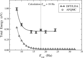
Figure 1: Convergence of the total energy of a phosphorus atom in a $14\times 14\times 14\,a_{0}^{3}$ unit cell. The OPIUM pseudopotential is used here. The convergence behavior is similar in both LDA and AF QMC methods. A constant shift is added to each data set for convenience, such that the converged energies are approximately $0$ eV and $0.5$ eV for LDA and AF QMC, respectively.

III.2 Supercell size convergence

Due to the periodic boundary conditions imposed in the calculations, the interactions between electrons in the simulation cell and their periodic images give rise to finite-size errors. To study the behavior of these errors, a series of LDA and AF QMC calculations were performed using different system sizes for cubic (and some tetragonal) shaped cells. Results for the phosphorous atom are shown in Fig. 2 as a function of supercell size. The AF QMC energies are seen to converge from below while the LDA energy converge from above. This is not surprising, since LDA treats the supercell Coulomb interaction differently from a many-body approach such as AF QMC. Fig. 3 shows that the total energy from AF QMC for the sulfur atom is nearly a linear function of $1/\Omega$ for this range of supercell sizes. At the largest $19\times 19\times 19\,a_{0}^{3}$ supercell size, the total energy is converged to within about $\sim 0.1$ eV.

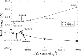
Figure 2: Convergence of the phosphorus total energy with respect to the inverse of the simulation cell volume $\Omega$. The triangles denote the results of LDA calculations while the solid circles denote those of the AF QMC. The OPIUM pseudopotential is used here.

Figure 3: Convergence of the AF QMC total energy with simulation cell size for Sulfur, plotted as a function of the inverse volume, from box sizes $12\times 12\times 12\,a_{0}^{3}$ through $19\times 19\times 19\,a_{0}^{3}$. The OAL pseudopotential is used here. The dotted line shows the fitting of the total energy as a linear function of $1/\Omega$. The data point shown at $1/\Omega=0$ shows the extrapolated energy at infinite box size.

To demonstrate the supercell size effect on the energy differences, Fig. 4 shows the calculated dissociation energy of P₂. The top panel shows the supercell size dependence of the dissociation energy, and the bottom panel illustrates the convergence error of P and P₂ energies for supercells ranging from $14\times 14\times 14\,a_{0}^{3}$ through $18\times 18\times 18\,a_{0}^{3}$. The total atom energy from different supercells deviates no more than $0.2$ eV from that of the largest supercell. The dimer total energy, on the other hand, shows stronger finite-size effect. Most of the finite-size error in the dissociation energy thus arises from the dimer energy. To avoid any irregular dependence of the energy on the aspect ratio (cubic vs. tetragonal supercells), only the cubic supercells were used in the extrapolation.

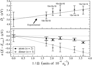
Figure 4: Phosphorus dissociation energy (top panel) and the total energies of P (times two) and P₂ (bottom panel) for different supercell sizes, computed using the OPIUM pseudopotential. The dissociation energy obtained with the largest simulation cell, $18\times 18\times 18\,a_{0}^{3}$ is within 0.1 eV of the experimental value of 5.08 eV (indicated by the horizontal dotted line in the top panel). $E_{\textrm{conv}}$ is the energy extrapolated to $1/\Omega\to 0$ (using cubic cells only).

In the ionization energy calculations, the supercells are charged $+|e|$ and $+|2e|$ for the $X^{+}$ and $X^{++}$ species, respectively. Charged supercells are ill-defined under periodic boundary conditions, so an additional neutralizing background charge is introduced to maintain charge neutrality Makov and Payne (1995); Makov et al. (1996). As discussed by Makov and Payne Makov and Payne (1995); Makov et al. (1996), a leading behavior, $q^{2}\alpha/2L$, arises from the self-interaction of the neutralizing charge with its periodic images, where $\alpha$ is the (supercell-dependent) Madelung constant, $q$ is neutralizing charge, and $L^{3}=\Omega$. Correction of the total energy by the leading term leads to more rapid size convergence. Figure 5 illustrates this effect. The bottom panel shows the slow convergence of the total energy with the system size in charged systems, while the upper panel shows the more rapid convergence after the correction has been made, i.e., the slowly convergent $q^{2}\alpha/2L$ contribution has been subtracted.

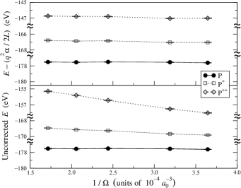
Figure 5: An illustration of the size effect in the calculation of charged atoms. The top panel shows the corrected total energies for P, P⁺ and P⁺⁺, while the bottom panel shows the uncorrected ones. Cell sizes used in this study are the same as in Fig. 4. The errorbars are smaller than the point size.

III.3 Trotter time step error

The Trotter error arises from neglecting higher order terms of the imaginary-time propagator, $e^{-\Delta\tau{{\hat{H}}}}$, when we apply the Trotter-Suzuki decomposition in Eq. (16). The Trotter error can be eliminated by extrapolation, as demonstrated in Fig. 6 for P, P⁺, and P⁺⁺. The results reported in the next section use either a linear extrapolation a fixed $\Delta\tau$ ($\sim 0.05$ Ha^-1) which is sufficiently small so that the Trotter error is well within the statistical error.

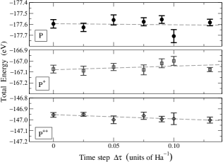
Figure 6: Trotter errors for P, P⁺ and P⁺⁺ energies (shown in the top, middle, and bottom panels, respectively) in a $14\times 14\times 14\,a_{0}^{3}$ simulation box. The data points at $\Delta\tau=0$ represent the Trotter extrapolation.

IV Results

Table 2 shows dissociation energies from planewave AF QMC calculations compared with experimental values and with LDA, GGA, HF, and diffusion Monte Carlo (DMC) calculated results. LDA trial wave functions were used in the molecular calculations, corresponding to the following electronic configurations: $\sigma^{2}_{\rm{3s}}\sigma^{*2}_{\rm{3s}}\sigma^{2}_{\rm{3p}}\pi^{4}_{\rm{3p}}$ for P₂, $\sigma^{2}_{\rm{3s}}\sigma^{*2}_{\rm{3s}}\sigma^{2}_{\rm{3p}}\pi^{4}_{\rm{3p}}\pi^{*2}_{\rm{3p}}$ for S₂, $\sigma^{2}_{\rm{3s}}\sigma^{*2}_{\rm{3s}}\sigma^{2}_{\rm{3p}}\pi^{4}_{\rm{3p}}\pi^{*4}_{\rm{3p}}$ for Cl₂, and $\sigma^{2}_{\rm{4s}}\sigma^{*2}_{\rm{4s}}\sigma^{2}_{\rm{4p}}\pi^{4}_{\rm{4p}}$ for As₂. All dimers except S₂ have “closed-shell” configurations in which all occupied orbitals are fully filled. All the calculations used OPIUM pseudopotentials.

Table 2: Calculated dissociation energies (in eV) using LDA, AF QMC, DMC, HF, and GGA methods. Experimental values are in the last column (with the zero-point energy removed). The AF QMC calculations used LDA trial wave functions, except for sulfur, where we have also used unrestricted HF trial wave functions. Values from the largest supercell are shown here, since convergence has been reached. The statistical errors are given in parentheses. The HF results are obtained from an in-house planewave based code. The AF QMC result for Si₂ is taken from Ref. Zhang and Krakauer, 2003.

	LDA	AF QMC (LDA)	DMC Grossman (2002)	HF	GGA Patton et al. (1997)	Expt. Lide (2002)
Si2	3.88	3.12(8)				3.21(13)
P2	5.97	5.19(16)	4.73(1)	1.74	5.22	5.08
S2	5.61	4.63(17)	4.31(1)	2.29	4.94	4.41
		4.48(19)
Cl2	3.12	2.78(10)	2.38(1)	0.67	2.76	2.51
As2	5.04	3.97(17)				3.96

Both restricted and unrestricted trial wave functions were tested in the AF QMC calculations, but there were no difference within statistical errors. (In restricted trial wave functions, the orbitals with minority spin are identical to the corresponding majority-spin orbitals.) Unrestricted HF trial wave functions were also used to calculate the dissociation energy of S₂, which has an open-shell configuration. As shown in Table 2, there is no difference within statistical errors.

The overall agreement between the AF QMC results and experiment is very good. The LDA and GGA slightly overestimate the dissociation energy, while the HF method significantly underestimates it. The heaviest dimer we calculated, As₂, is also in excellent agreement with experiment and compares favorably with results from other quantum chemistry methods Sakai and Miyoshi (1997); Mochizuki et al. (1994).

Table 3: First and second ionization energies for several atoms, in eV. We employ two pseudopotentials, the LDA-based OPIUM pseudopotential and HF-based effective core potential (OAL). In most cases, we use LDA trial wave functions (see text). The LDA calculations were done using ABINIT. The HF results were obtained using an in-house HF program for OPIUM pseudopotential and GAUSSIANFrisch et al. (2002, 2004) for OAL. Experimental values are taken from Ref. Lide, 2002. The quantity $\Delta\textrm{IP}$ below is the difference between the AF QMC-calculated and the experimental ionization energies, for which we show the average and r.m.s. average over all the species shown here.

		IP ($X\rightarrow X^{+}$)									IIP ($X\rightarrow X^{++}$)
	Pseudo	HF		LDA		AF QMC		Expt			HF		LDA		AF QMC		Expt
Al	OAL			5.	88	5.	88(2)	5.	99				24.	46	24.	66(2)	24.	81
Si	OPIUM					8.	18(2)	8.	15						24.	59(4)	24.	50
P	OPIUM	9.	97	10.	57	10.	74(6)	10.	49		29.	41	30.	42	30.	79(6)	30.	26
	OAL	9.	94	10.	41	10.	61(3)				29.	11	29.	97	30.	28(6)
S	OPIUM	9.	33	10.	45	10.	09(7)	10.	36		32.	42	33.	85	34.	16(7)	33.	67
	OAL	9.	21	10.	35	10.	08(2)				32.	06	33.	51	33.	61(2)
Cl	OPIUM	11.	69	13.	12	12.	96(11)	12.	97		34.	36	36.	92	36.	76(10)	36.	78
	OAL	11.	76	13.	02	12.	89(6)				34.	30	36.	64	36.	25(6)
$\langle\Delta\textrm{IP}(\textrm{OPIUM})\rangle$						0.	00								0.	27
$\langle\Delta\textrm{IP}(\textrm{OPIUM})\rangle_{\mathrm{rms}}$						0.	19								0.	36
$\langle\Delta\textrm{IP}(\textrm{OAL{}})\rangle$						–0.	09								–0.	18
$\langle\Delta\textrm{IP}(\textrm{OAL{}})\rangle_{\mathrm{rms}}$						0.	16								0.	28

We show in Table 3 the first and second ionization energies of Al, Si, P, S and Cl. For comparison, experimental values and results from LDA and HF calculations are also shown. The AF QMC calculations are performed using both the OPIUM and OAL pseudopotentials together with LDA trial wave functions, except for sulfur with the OAL pseudopotential, where HF trial wave functions are also used. Again, no statistically significant dependence on the trial wave function is seen. The tabulated results are converged with respect to size effects, which are negligible compared to the QMC statistical error for supercells larger than $16\times 16\times 16\,a_{0}^{3}$.

Ionization energies obtained using the LDA are generally in very good agreement with experiment, and the present results are consistent with this, with deviations typically within $0.1$ eV for IP and $0.3$ eV for IIP, regardless of which pseudopotential is used. The HF method results in larger deviations of $0.5$–$1.3$ eV compared to the experiment.

AF QMC results for Al and Si are in good agreement with experiment, and for Si the agreement is comparable to that obtained using DMCLee and Needs (2003), $8.166(14)$ eV and $24.444(22)$ eV for IP and IIP, respectively. For P, S, and Cl, however, the agreement between AF QMC and experiment is not as uniform. In particular, there is a significant dependence on the choice of the pseudopotential. For P and S, the AF QMC ionization energies are better estimated using OAL, while for Cl, OPIUM pseudopotential gives better results. We will discuss this dependence in the next section. Agreement between the best AF QMC and experiment values is in general very good.

V Discussion

For dissociation energies, the agreement between AF QMC and experiment was uniformly very good. The appearance of larger discrepancies between AF QMC and experiment for ionization energies is somewhat surprising. The AF QMC calculations above were systematically converged with respect to finite size effects, Trotter time step error, and planewave basis size. Two remaining possibilities, errors arising from the use of the phaseless approximation and errors due to the use of pseudopotentials, are discussed in this section.

Our overall experience with the phaseless AF QMCZhang and Krakauer (2003); Zhang et al. (2005); Al-Saidi et al. (2006a, b); Purwanto and Zhang (2004) suggests that the error due to the phaseless approximation itself is typically small. Recent AF QMC calculations using a Gaussian basis Al-Saidi et al. (2006b) show that, in a variety of atoms and molecules, the AF QMC agrees well with experiment or high-level quantum chemistry methods such as the coupled cluster with single and double excitations and perturbative corrections for triple excitations [CCSD(T)]Čízek (1966, 1969); Purvis III and Bartlett (1982); Pople et al. (1987). Open-shell systems such as P⁺, P⁺⁺, S, S⁺⁺, Cl, and Cl⁺, where the $p$ shell is neither half- nor fully-filled, tend to be more difficult to treat in general Stanton and Gauss (2005). In these cases a single-determinant trial wave function breaks the symmetry by using only one of the degenerate states, and the phaseless approximation could affect the accuracy of the results. Some indication of this may be present in our results (see Table 3) where larger errors are observed for energy differences between half-filled and “open-shell” systems, such as the P⁺ ionization energy. It is possible to use multideterminant trial wave functions in these cases. We have done several tests, in which we “symmetrize” the trial wave function, resulting in a linear combinations of three different determinants. This is designed to equally treat the $p_{x}$, $p_{y}$, and $p_{z}$ orbitals in the open shell. However, there seems to be no observable improvement over the single-determinant trial wave function at the level of statistical accuracy in this paper.

To isolate and quantitatively evaluate the errors due to the phaseless approximation on the second-row atoms studied here, we performed calculations with both AF QMC and CCSD(T) methods for Cl, Cl⁺, and Cl⁺⁺, using identical Gaussian basis sets and the OAL pseudopotential. (The OAL pseudopotential was chosen since its form is already compatible with standard quantum chemistry programs.) Thus, both the AF QMC and CCSD(T) methods are applied to the same many-body Hamiltonian, expressed in the Hilbert space spanned by the selected Gaussian basis set. The CCSD(T) method is approximate but is known to be very accurate in atoms and in molecules near equilibrium. For the comparison, we employed an uncontracted aug-cc-pVDZWoon and Dunning, Jr. (1993); PNL basis set, where Gaussian functions with exponents larger than $98$ are removed, resulting in a $(7s7p2d)$ basis set. As shown in Table 4, the AF QMC and CCSD(T) absolute total energies agree to within $0.07$ eV, and their ionization energies agree to within $0.04$ eV. These results indicate that the intrinsic error due to the phaseless approximation in the above planewave calculations is likely also small, consistent with previous experience with phaseless AF QMCZhang and Krakauer (2003); Zhang et al. (2005); Al-Saidi et al. (2006a, b); Purwanto and Zhang (2004). This suggests that errors due to the use of pseudopotentials are largely responsible for the deviations in ionization energies noted above.

Table 4: Calculated total energies ($E$) and ionization energies (IP) for Cl, using AF QMC with a Gaussian basis together with the corresponding CCSD(T) results, using identical basis sets. The OAL pseudopotential is used with a double-zeta quality $(7s7p2d)$ Gaussian basis set. All energies are in eV. Since CCSD(T) is known to be accurate for atoms, differences compared to Gaussian-based AF QMC provide an estimate of errors due to the phaseless approximation in AF QMC.

	AF QMC					CCSD(T)
	$E$		IP			$E$		IP
Cl	–403.	91(1)				–403.	96
Cl+	–391.	37(1)	12.	54(2)		–391.	44	12.	51
Cl++	–368.	43(1)	35.	49(2)		–368.	43	35.	53

The pseudopotentials used here were generated using independent-electron HF or DFT mean-field type calculations of atomic reference systems. While the transferability of these pseudopotentials to HF or DFT calculations of molecules or solids is well understood, their accuracy in many-body calculations is more problematic.Shirley and Martin (1993); Lee and Needs (2003) The dependence of the AF QMC results in Table 3 on the choice of pseudopotentials is consistent with this.

To estimate the pseudopotential errors in our AF QMC calculations and to obtain insight into their origin, we have carried out several additional calculations. We first performed pseudopotential and all-electron (AE) CCSD(T) calculations to estimate the transferability of the pseudopotential in a many-body context. First and second ionization energies for P, S, and Cl atoms were calculated using both methods. The coupled-cluster calculations were performed using the GAUSSIAN98 and GAUSSIAN03 packagesFrisch et al. (2002, 2004). To eliminate basis set convergence errors, we performed a series of AE calculations using the aug-cc-p$w$CV$x$Z basis setsWoon and Dunning, Jr. (1993); Peterson and Dunning, Jr. (2002); PNL , where $x=$ D, T, Q for double, triple, and quadruple zeta basis sets, respectively. The infinite-basis estimate of the total energy, $E_{\infty}$, is then obtained using extrapolationFeller and Peterson (1998)

$$\begin{split}E_{\infty}\approx E_{x}-be^{-cx}\,,\end{split}$$ (32)

where $x$ is $2,3,4$ for double, triple, and quadruple zeta basis sets, respectively, and $b$ and $c$ are fitting parameters. We then take the difference of the extrapolated energies as the ionization potential shown in Table 5. For the pseudopotential calculations, the OAL ECP is used. Here we use the aug-cc-pV$x$Z basis setsWoon and Dunning, Jr. (1993); PNL that are fully uncontracted, and again we use the extrapolation scheme in Eq. (32).

Table 5: Estimates of pseudopotential errors: CCSD(T) results for the first and second ionization energies of P, S, and Cl. All energies are in eV. OAL and AE results are shown together with the error in the ionization energy due to the pseudopotential, $\Delta\textrm{IP}_{\mathrm{psp}}$.

		IP ($X\rightarrow X^{+}$)									IIP ($X\rightarrow X^{++}$)
		OAL		AE		$\Delta\textrm{IP}_{\mathrm{psp}}$		Expt.			OAL		AE		$\Delta\textrm{IIP}_{\mathrm{psp}}$		Expt.
P		10.	48	10.	47	0.	01	10.	49		30.	13	30.	18	–0.	05	30.	26
S		10.	24	10.	29	–0.	05	10.	36		33.	64	33.	64	0.	00	33.	67
Cl		12.	92	13.	05	–0.	13	12.	97		36.	51	36.	77	–0.	26	36.	78

The CCSD(T) results for AE and OAL calculations are presented in Table 5. AE CCSD(T) ionization energies are seen to be in excellent agreement with experimental values. [We note that AE calculations using aug-cc-pCV$x$Z basis set (a variation of aug-cc-p$w$CV$x$Z) yield almost identical result, where the estimated IP differs by $\lesssim 0.03$ eV, and IIP by $\lesssim 0.07$ eV.] The difference between the AE and OAL results provides an estimate of the error due to the pseudopotential in many-body calculations. The results in Table 5 indicate that the OAL pseudopotential tends to underestimate the ionization energies. The rms error attributable to the pseudopotential is about $0.12$ eV. This is not negligible compared to the overall AF QMC error, which is $\langle\Delta\textrm{IP}(\textrm{OAL{}})\rangle_{\mathrm{rms}}=0.25$ eV for P, S, and Cl first and second ionization energies.

An additional possible source of pseudopotential error in the planewave AF QMC calculations is the use of the fully nonlocal, separable Kleinman-Bylander (KB) construction of the pseudopotential. For example, the OAL ECP is defined in the usual semilocal form, which is used in quantum chemistry programs:

$$\begin{split}\hat{V}_{\textrm{ei}}^{\textrm{(SL)}}(\mathbf{r})=\sum_{l,m}|{{Y_{lm}}}\rangle V_{l}(r)\langle{{Y_{lm}}}|\,.\end{split}$$ (33)

where $V_{l}(r)$ is the angular-momentum-dependent potential. For efficient use in the planewave calculations, it is common to express this pseudopotential in the fully nonlocal separable KB form shown in Eq. (31a). While the KB and semilocal forms are identical when they act on the reference atomic state, the KB form can differ for other states.

To investigate the effect of pseudopotential KB formation, we perform LDA Perdew and Wang (1992) calculations with the OAL pseudopotential: (1) planewave basis calculations with the KB form of the OAL using the ABINIT package (calculations are converged with respect to $E_{\textrm{cut}}$ and box size), and (2) local basis calculations with the semilocal form of the OAL using GAUSSIAN98 (again we use the sequence of aug-cc-pV$x$Z basis sets to extrapolate to the infinite basis limit). The OAL pseudopotential was converted to the KB form using pseudo-orbitals obtained in an LDA calculation for the neutral atom. For the purpose of constructing the fully nonlocal projectors, the effects of using LDA rather than HF pseudo-orbitals are not expected to to be significant. In both methods, the total-energies are converged to within $0.5$ mHa ($\approx 0.01$ eV). Table 6 presents the results for the Cl ionization energies. The OAL pseudopotential expressed in the KB form tends to underestimate the LDA total energies, with the discrepancy increasing with the ionization state. Ionization energies are thus underestimated by up to $0.15$ eV. The same trend is observed in the calculated planewave AF QMC ionization energies compared to experiment, which indicates that the KB form may contribute errors of the order of $0.1-0.2$ eV for Cl using the OAL pseudopotential. It is clear that the quality of the pseudopotential is crucial for obtaining accurate results with AF QMC.

Table 6: LDA calculations of chlorine energies, the Kleinman-Bylander (KB) and semilocal (SL) forms of the OAL pseudopotential. The programs used are indicated in parantheses, and all energies are in eV.

	Kleinman-Bylander					Semilocal
	(ABINIT)					(GAUSSIAN98)
System	$E$		IP			$E$		IP			$(E^{\mathrm{KB}}\!-\!E^{\mathrm{SL}})$
Cl	–403.	798				–403.	752				–0.	05
Cl+	–390.	842	12.	956		–390.	701	13.	051		–0.	14
Cl++	–367.	217	36.	581		–367.	021	36.	731		–0.	20

These test calculations are limited in scope. Small systematic errors may well be still present, for example from the planewave size-extrapolations, from Gaussian basis set extrapolations, and from approximations inherent in coupled cluster calculations at the CCSD(T) level. They suggest, however, a rather consistent picture for understanding the AF QMC results in Table 3. Pseudopotential errors due to different origins appear to be the main cause for the discrepancies with experimental values. When such errors are removed, it seems that the accuracy of the planewave AF QMC is at the level of 0.1 eV.

Table 7: Phosphorus ionization and dissociation energies for P⁺, P⁺⁺, and P₂ computed using LDA, HF, AF QMC, and CCSD(T) methods, shown below in eV. AE results are provided to benchmark the pseudopotentials. The numbers shown in boldface are those closest to the AE results (for LDA and HF) or the experimental values (for AF QMC).

PSP	LDA		HF		AF QMC		CCSD(T)
IP (P $\rightarrow$ P+)							expt = 10.	49
OPIUM	10.	57	9.	97	10.	74(6)
OAL	10.	41	9.	94	10.	61(3)	10.	48
AE	10.	53	9.	91			10.	47
IIP (P $\rightarrow$ P++)							expt = 30.	26
OPIUM	30.	42	29.	41	30.	79(6)
OAL	29.	97	29.	11	30.	28(6)	30.	13
AE	30.	37	29.	08			30.	18
$D_{e}$ (P${}_{2}\rightarrow 2$P)							expt = 5.	08
OPIUM	5.	97	1.	74	5.	19(16)
OAL	5.	29	0.	98	3.	88(8)	4.	39
AE	6.	18	1.	65			4.	98

Since the quality of a pseudopotential within HF and LDA can be easily determined (by its ability to reproduce AE results), it is interesting to see how well this correlates with the performance of the pseudopotential in a many-body calculation. In Table 7 we show various energies obtained from LDA, HF, AF QMC, and CCSD(T) calculations in phosphorus. (Similar trends also hold for sulfur and chlorine.) Results are shown using the OPIUM and OAL pseudopotentials, together with AE results for independent-electron and CCSD(T) methods. In the LDA calculations, the LDA-based OPIUM potential performs uniformly better for all quantities. In the HF calculations, the HF-based OAL pseudopotential performs well, except for the dissociation energy. (As mentioned earlier, the OAL pseudopotential lacks a $d$ projector in its construction, which results in poor molecular energies.) Overall, the HF method appears to give a better indication of pseudopotential performance with AF QMC. In the chlorine second ionization energy, for example, HF predicts that the OPIUM pseudopotential performs better than the OAL pseudopotential: IIP${}_{\textrm{HF, OPIUM}}=34.37$ eV, IIP${}_{\textrm{HF, OAL{}}}=34.30$ eV, compared to IIP${}_{\textrm{HF, all-electron}}=34.36$ eV. AF QMC results in Table 3 show a similar trend. We also note in Table 3 that the LDA-based OPIUM pseudopotentials tend to overestimate the ionization energies, while the OAL pseudopotentials do the opposite. The tabulated rms averages suggest that the performance of AF QMC with the LDA-generated OPIUM pseudopotential varies more widely across different atomic species, especially in the second ionization energies. The HF-generated OAL ECP, on the other hand, performs more consistently and yields better agreement with experiment in the majority of species studied here. Testing pseudopotentials using Hartree-Fock calculations may, therefore, be a useful predictor of their performance in the many-body AF QMC method.

VI Summary

We have presented electronic structure calculations in atoms and molecules using the phaseless AF QMC method with a planewave basis and norm-conserving pseudopotentials. Various algorithmic issues and characteristics were described and discussed in some detail, and we have illustrated how the AF QMC method can be implemented by utilizing standard DFT planewave techniques. The structure of the AF QMC calculation is an independent collection of random walker streams. Each stream resembles an LDA calculation, which makes the overall computational scaling of the method similar to LDA calculation with a large prefactor. This makes the AF QMC approach more efficient than explicit many-body methods. All of the reported results were obtained using single-determinant trial wave functions, directly obtained from either LDA or HF calculations. This reduces the demand for wave function optimization in QMC and is potentially an advantage. The method also offers a different route to the sign problem by carrying out the random walks in Slater determinant space. Because our method is based in Slater determinant space, any single-particle basis can be used.

Results for the dissociation and ionization energies of second-row atoms and dimers in Group 3A-7A, Al, Si, P, S, Cl, as well as the As₂ dimer, were presented using the planewave-based phaseless AF QMC method. The effects of the phaseless approximation in AF QMC were studied, and the accuracy of the pseudopotentials were examined. Comparisons were made with experiment and with results from other methods including the DMC and CCSD(T). Errors due to the phaseless approximation were found to be small, but non-negligible pseudopotential errors were observed in some cases. In addition to pseudopotential errors that arise due to their construction in mean-field type DFT or HF calculations, possible errors in ionization energies arising from the separable Kleinman-Bylander form of the pseudopotentials were also observed. With the appropriate pseudopotentials, the method yielded consistently accurate results.